
Acoustic emission sensors for assessing and monitoring civil infrastructures
M. Meo, University of Bath, UK
Abstract:
This chapter presents a review of recent developments in acoustic emission (AE) techniques applied to civil structures. It recapitulates the significant milestones achieved by previous researchers, including various methods and models developed in AE testing of civil structures. The aim is to provide an overview of the use of AE techniques for structural health monitoring of civil structures carried out over the years. Basic principles are introduced, followed by acoustic source localization and severity assessment methods. An overview of AE equipment technology is then presented with field application of AE. Finally, current and future challenges are discussed.
Key words
acoustic emission monitoring; acoustic detection; concrete; Kaiser effect; non-destructive evaluation
6.1 Introduction
As the infrastructure ages, civil structures reach the end of their economic lives. Replacement costs and life extension become critical issues and reliable inspection-based maintenance protocols ensure their safe, reliable and economic operation without undue risk to public health and safety. The classical fail-safe design and maintenance approach does not tolerate any known crack or defects, and it has had major financial implications in ensuring integrity of structures. This has forced civil infrastructure operators to adopt a new approach used in the aerospace industry, whereby flaws or damage are tolerated as long as they do not compromise a structure's ability to perform its function. Significant cost savings result by detecting defective parts before the end of their design life and avoiding unnecessary replacement of sound components. Visual inspection and non-destructive testing (NDT) is the basis for the retirement-for-cause approach. NDT examines materials or components in ways that do not impair future usefulness and serviceability and is used to detect, locate, measure, and evaluate flaws/dam- age and to assess integrity. Various NDT technologies, such as radiographic methods, ultrasonic-based methods, acoustic emission (AE) techniques, to name a few, are used to monitor civil structures. Each NDT technique has both advantages and disadvantages with regard to cost, speed, accuracy, and safety, and the choice of a technique is strictly correlated with the kind of structure to be analysed and the data to be extracted.
AE is a significant resource with a specific role to play in the spectrum of maintenance resources both in its own right and as a complement to other monitoring technologies. AE is defined as the transient stress waves generated by the rapid energy from localized sources within a structure. After originating, stress waves travel to the surface and become surface waves. The surface mechanical waves can be detected by sensors. These AE bursts can be used both to locate cracks and to evaluate their rate of growth as a function of the applied stress. One of the main advantages of AE methods is that they detect and locate cracks in one measurement. In addition to this, since acoustic waves propagate through the structure, they can provide remote monitoring of inaccessible areas and the ability to monitor with a minimum number of sensors. This is in contrast to most other NDT methods, which require point-by-point inspection and are therefore limited to accessible areas of a structure. However, AE testing does not determine the size of cracks – it allows a reduction of the area to be scanned by other non-destructive test techniques to quantify problems in the areas identified by AE testing. Further analysis by fracture mechanics can be used to determine the severity of defect from the structural integrity point of view.
6.2 Fundamentals of acoustic emission (AE) technique
AE monitoring is a passive monitoring technique aimed at detecting acoustic stress waves generated in materials that arise from the rapid release of strain energy from micro-structural changes in a material.1 The sources of AE are initiation/growth of cracks, yielding, failure of bonds, fibre failure, delamination in composites, etc. Most of the sources of AEs are damage-related; thus, the detection and monitoring of these emissions are commonly used to predict material failure. Localized energy release travelling as elastic waves move to the surface and, if the waves are of sufficient amplitude, are detected by transducers attached to the surface of the specimen provided. Acoustic stress wave detection is a complex task, since it is strongly related to the main features of propagating stress waves, attenuation, effects of multiple paths, source location algorithm criterion, etc.1
In contrast to other NDT/structural health monitoring (SHM) methods, AE is usually applied during loading to verify the occurrence of AE, while most others are applied before or after loading of a structure.
The AE technique is a procedure for monitoring and analysing of AE, whereas AE testing is a method to test the presence or absence of AE activity. The AE method analyses the evolution of cracks and estimates the released strain energy during their propagation in structural members.
The AE waves may consist of only a single transient event, or be composed of a number of discrete cracks and microcracks, each producing an AE, depending on the material and the stress regime failure.
Typical AE waves generated through sudden release of energy are usually of low amplitude. In general, AEs can be classified into primary and secondary emissions. Primary emissions are those originating from within the material of interest, while secondary emissions refer to all other emissions generated from external sources. Therefore, in AE monitoring it is vital to reduce the noise mixed up with signal parts related to the fracture process. To enhance the signal-to-noise ratio in AE analysis there is a need to employ efficient filter techniques.
The typical AE process step consists of the following steps and actions reported in Table 6.1.
Table 6.1
| Step | Action |
| 1. Structure under in-service loads | Produce stress |
| 2. Source mechanisms | Release elastic energy |
| 3. Wave propagation | Direct wave path from the source to the sensor and reflections |
| 4. AE transducers | Stress waves are converted into an electrical AE signal |
| 5. Acquisition of measurement data | Converting the electrical AE signal into data with amplification and filtering |
| 6. Data post-processing | Convert waveforms into meaningful parameters |
| 7. Integrity evaluation | Assess damage based on processed data |
Basically, the AE monitoring technique detects a crack growth process as it occurs.
6.3 Interpretation of AE signals
A typical burst AE signal and the typical parameters used for AE techniques are shown in Plate III in the colour section between pages 294 and 295.2 In the AE method, also called ring-down counting or event-counting, when the amplitude of stress waves acquired by the AE transducer is over a certain threshold level (measured in volts), an AE event is captured. The peak of the signal defines the amplitude of the AE event, and the AE count is the number of times the wave crosses the threshold.
The amplitude is closely related to the magnitude of the source event, and it is an important parameter in determining the system's detectability.
The duration of an AE event is defined by the time period between the rising edge of the first count and the falling edge of the last count, and the rise time is the time period between the rising edge of the first count and the peak of the AE event. It must be noted that 'counts' are strongly dependent on the operating frequency and clearly the employed threshold. The area under the envelope of the AE event is the energy. It is usually more appropriate to analyse the energy to interpret the magnitude of source event over counts because it is sensitive to the amplitude as well as the duration, and less dependent on the operating frequencies and voltage threshold.
AE technique involves recording the stress waves by means of sensors placed on the surface of the structure and subsequent analysis of the recorded signals to locate and gather information about the nature of the source of emission.
6.4 AE localization methods
Traditional AE uses only some of the features of AE signals, due to the main limitations of available sensors as well as data-capturing and analysis capability. Recent progress has been made in transducer technology, wide-band, acquisition systems, etc. New AE sensors able to capture the whole wave- form have been developed, allowing accurate localization as well as characterization of the nature of AE sources from the waveform captured.
Localization of the AE source is a complex procedure for civil structures due to the large area needed to be monitored, and the distortion of the waveforms due to presence of different materials, non-linear effects, tapered sections, etc. It is possible to solve inverse wave-propagation problems to identify the source of the AE signals detected using one or more sensors by analysing the whole waveform.
A typical conventional AE set-up consists of many sensors distributed around potential source locations to be assessed. AE source localization is an inverse problem. By measuring the arrival time differences of the elastic wave emitted by the AE sources fracture at each sensor, the source location can be calculated by assessing the AE event origin time and the AE source coordi- nates (x0, y0, z0). The computed location corresponds to the point in space and time where the crack growth is initiated. Generally a point source is assumed.
In most of the localization methods, the onset times, the coordinates of each corresponding sensor and the velocities of the compressional and shear wave for bulk materials or group velocity (dispersion curves) for thin walled structures are needed.
While for homogeneous and isotropic material the direct ray path between source and receiver can be used for calculation of the source location, in the case of layered materials or heterogeneous and anisotropic material, directional properties of stress wave propagation must be taken into consideration for an accurate localization.
One of the most difficult tasks to estimate source location is the determination of the time of arrival (TOA) or onset picking. The simplest method for TOA estimation is to use an amplitude threshold picker. However, a pure threshold approach would not be applicable to signals with small amplitudes and/or signals with high noise levels.
Another approach used in the seismic application is to model the signal as an autoregressive process,3 whereby a time series is divided into stationary segments modelled as an autoregressive process (Akaike Information Criterion, abbreviated as AIC). This approach developed has been transferred to the AE field by Kurz et al.4
Another common TOA estimation method is cross-correlation, whereby the correlation between two signals acquired by two sensors is defined by the following formulas:
[6.1]
where Ssensor 1 (τ) is the time history of the acquired waveform. Then the time difference is:
[6.2]
An example is reported in Fig. 6.1.
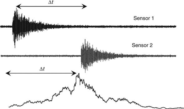
The sensor 1 in this approach is commonly termed the master sensor, which will help in calculating the time difference that will be used for the localization approach. The cross-correlation function gives a measure of the similarity of two time series shifted along each other. The maximum value of f(t) indicates the maximum correlation of the two signals gained at the time shift t. A detailed comparison of these techniques for TOA estimation strategies can be found in Reference 4. Other techniques include using wavelets, which were employed for the aerospace sector and applied with success. A detailed discussion can be found in References 5 and 6.
There are a number of methods to localize the source of AEs. In 1-D, by knowing the propagation velocity V, the distance D between the two sensors, the onset time at each sensor or the time difference Δt between the arrival time at sensor 1 and 2 as explained in Fig. 6.1, the distance of the source xsource can be calculated by this formula, as shown in Fig. 6.2.
[6.3]
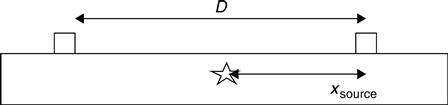
This approach can be applied to structures such as pipes. To perform a 2-dimensional (2-D) localization there is the need to determine the coordinates xsource and ysource of the AE source. For 2-D structures, where the thickness is small compared to other geometrical entities, and for waves with wavelengths longer than the thickness of the structure, group velocities of plate or Lamb waves have to be used for localization. At least three sensors are needed for a 2-D localization. Assuming constant velocity and three measured arrival times t1, t2 and t3 of the wave, at three different sensors, the AE source can be calculated by the hyperbola7 or circle method8 as the intersection of the three curves as shown in Fig. 6.3.
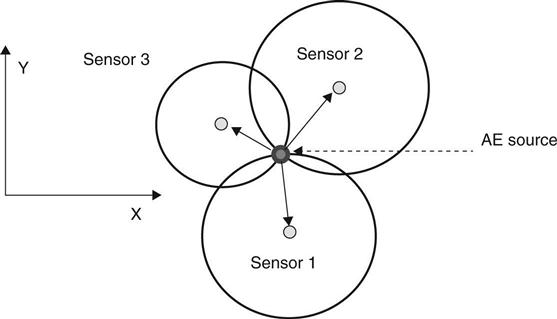
Because of measurement error, to improve localization accuracy extra sensors may be needed. This technique can be extended to 3D structures, but there is the need to have one extra sensor to detect also the zsource. It must be noted that these techniques are valid under the assumption of homogenous and isotropic materials and the AE source can be assumed as a point source. Due to the presence of different sources (noise, etc.), the determination of the arrival times can lead to incorrect AE source estimation. One particularly important issue when recording AE events is background or environmental noise, and particular care is needed during the experiment. A solution is to set the frequency range of the measurement above that of the environmental noise, achieved by grounding the equipment. Then a band-pass filter can be used to reduce/eliminate spurious sources of noise. Generally, it is necessary to perform error analysis to assess the accuracy and reliability of any localization result. The bandwidth from several kHz to several 100 kHz or 1 MHz is usually used in AE measurements. For layered media the group velocity is direction dependent, and therefore complex algorithms are necessary to locate the source.
Recently Meo et al.9,10 suggested a localization method to detect the source location in reverberant complex composite structures using only one passive sensor. This technique was based on the time reversal acoustic method applied to a number of waveforms stored in a database containing the impulse response (Green’s function) of the structure. The proposed method allowed the optimal focalization of the AE source in the time and spatial domain overcoming the drawbacks of other ultrasonic techniques. This was mainly due to the dispersive nature of guided Lamb waves, as well as the presence of multiple scattering and mode conversion that can degrade the quality of the focusing, causing poor localization. Conversely, by using the benefits of a diffuse wave field, the imaging of the source location was obtained through a virtual time reversal procedure, which did not require any iterative algorithms and a priori knowledge of the mechanical properties and the anisotropic group speed. The efficiency of this method was experimentally demonstrated on a stiffened composite panel. The results showed that the source location was retrieved with a high level of accuracy in any position of the structure, with a maximum error of less than 3%.
6.5 Severity assessment
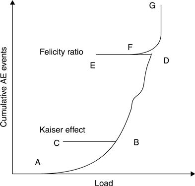
A material is known to produce acoustic waves only after until the previous load peak is achieved or exceeded. This phenomenon, named the ‘Kaiser’ effect, can be seen in the load vs AE plot (Fig. 6.4). AE is generated when load is increased (AB), but as the load lowered (BC) and raised again (CB), AE can be recorded until the previous load maximum is exceeded. As load is increased again the cumulative AE events increase (BD), and stop as the load is lowered for the second time (DE). On further increase of the load, a different emission pattern is observed: AE is observed at a lower load than the previous maximum load is attained (F). Emission continues as the load is increased (FG). The Kaiser effect can be observed if no permanent damage within the specimen has occurred.11 In the presence of permanent damage (load D), AE activity starts to be observed even under lower stress (load D) than that of the maximum stress experienced, and this new condition is known as the Felicity effect. Basically, at point F, the applied load is high enough to cause significant emissions even though the previous maximum load (D) was not reached. The significance of this effect and its related damage is defined by a Felicity ratio, which is the load at which AE events are first generated upon reloading divided by the previously applied maximum load. Insignificant flaws tend to show the Kaiser effect, while structurally significant flaws tend to show the Felicity effect. The latter has been successfully applied in monitoring damage progression in composite materials.11
Analysis of the above mentioned conventional AE parameters can provide qualitative results. In order to evaluate the level of deterioration, quantitative damage assessment is necessary. Golaski12 suggested the use of statistical analysis-based parameters to measure deterioration of materials applied to concrete bridges. They proposed to describe the intensity of an emission source by calculating the historic and severity index taken during the proposed loading. The historic index (HI) compares the signal strength of the most recent hits to all the hits defined by:
[6.4]
 [6.4]
[6.4]
where H(t) is the HI at time t, N is the number of hits up to and including time t, SOi is the signal strength of the i-th event and K is an empirically derived factor that varies with the number of hits. The values of K are dependent on materials and N.13
The severity index (Sr) is defined as the average signal strength for the J events having the largest numerical value of signal strength, and is defined by the following equation:
[6.5]
where Sr is severity and SOi is the signal strength of the i-th event as above. This procedure was first introduced in Reference 13 for damage evaluation in composite tanks and pipelines.
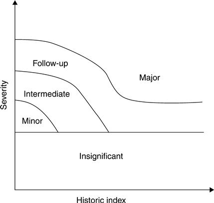
To determinate the intensity, the maximum HI and severity values are collected by each sensor and plotted on a chart. An example is shown in Fig. 6.5 where the severity index and maximum value of HI are plotted and the intensity chart is divided into zones with different levels of damage.14 The location of the sensor point in the chart will indicate the level of damage.
Depending on the type of cracks, different types of AE signals with varying frequency ranges and amplitudes are generated. Microcracks are characterized by a large number of events of small amplitude, in contrast to macrocracks where fewer events with larger amplitude are generated. In open cracks, where most of the energy has already been released, many AE events are created with small amplitude. Furthermore, while shear cracks create smaller amplitude signals, tensile cracks spawn large amplitude AE. The b-value analysis15 takes these factors into account and is used as an alternative way to process and interpret data recorded during a local AE monitoring. The b-value analysis derives from seismology, where the following formula relates the number of events to peak-amplitude of AE events:
[6.6]
where ML is the magnitude of an event on the Richter scale, N is the number of events with magnitudes in the range ML ± ΔM/2, and a and b are empirical constants. This formula can be adapted for AE by substituting ML with AdB that represent the peak-amplitude of the AE events in decibels. The b-value is calculated as the negative slope of log-linear plot of the frequency-magnitude distribution of AE. The b-value changes systematically with the different stages of fracture growth so it can be used to estimate the development of fracture process.15 When microcracks occur in the early stages of damage, the b-value is high but becomes low when macrocracks begin to occur.15 This fact makes the b-value an indicator of the presence of damage when stresses are redistributed and damage becomes more localized.16
6.6 AE equipment technology
The basic AE techniques consist of AE wave sources, the detection equipment used to capture AE signals, and the processing and interpretation of the collected data. An AE wave is an elastic wave, a combination of longitudinal, transverse, reflected waves, etc., with a broadband frequency range (kHz to MHz), generated by the release of energy by the formation of a microcrack. Most traditional AE sensors consist of a piezoelectric (lead zirconate titanate (PZT)) device that transforms motion produced by an elastic wave into an electrical signal.
The frequency response of the transducer is dependent on the dimension of the PZT, and the sensitivity of an AE transducer depends on its mode of operation and construction (resonant or broadband). Piezoceramic resonant transducers tend to have high sensitivity near resonance. Broadband piezoceramic transducers are sensitive to a wide range of frequencies, although they generally have lower sensitivity than resonant transducers.
In the selection of the appropriate AE transducer, the sensitivity and frequency response should be taken into consideration based on the purpose and sensitivity required for the investigation.
For thin structures, a higher frequency transducer should be used, since wave- length is determined from the velocity divided by frequency, while for materials with high attenuation, low resonance AE transducers should be used.
Typically, the signal from the transducers is preamplified, converted into electric voltage, filtered to eliminate unwanted frequencies and processed in a data acquisition system. The preamplifiers can be integrated with the sensor or connected to it.
While the frequency spectrum of the AE signal wave is mainly dependent on the transducer characteristics, materials and wave path, the AE signal waveform is affected by thickness dimension; for example, when the wavelength is greater than the thickness, Lamb wave modes propagate and the maximum amplitude is not determined by surface waves. Knowledge of wave modes and their characteristics is particularly important when the AE source needs to be localized. To minimize energy transfer loss from the surface of the material, appropriate couplant should be used.
In presence of different acoustic sources, unidirectional sensors and sensors, more sensitive to in-plane wave modes, should be used, especially for bridge monitoring.17
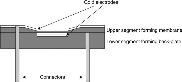
Other types of sensors include capacitive transducers, shape memory alloys and optical fibre sensors.18,19 A capacitive AE micromachined transducer20 was recently produced from polymer material using microstereolithography (Fig. 6.6). With this cost-effective approach, the sensor architecture could be shaped to conform to complex geometries, ideal for in situ inspection. An electroded vibrating membrane was placed over an air cavity, at the bottom of which a second electrode was placed. A force (acoustic generation) on the membrane was generated by applying a voltage. This showed that when introducing a DC bias, the device could also be used as a receiver, like a conventional condenser microphone.
Recently, capacitive-type AE sensors, based on multi-user micro-electro-mechanical systems (MEMS) processes (MUMPS), have attracted the attention of researchers.21,22 MEMS technology is a collection of methods and techniques to fabricate microscale systems. The advantages of MEMS devices include miniaturization of systems, multiple systems on one chip, and reduced cost due to batch processing. MEMS devices are sometimes manufactured by a process known as surface micromachining, during which structures are built up through a process of depositing, patterning and etching different materials on the chip substrate. Typically, the substrate is silicon, and structures are formed out of polysilicon. MEMS technology makes it possible to locate multiple transducer designs on a small area, which can provide additional information about the source. In principle, MEMS technology also invites the development of sensors integrated with signal processing. However, often MEMS-based sensors have limited sensitivity and must be operated in a vacuum for practical use. In addition, most MEMS sensors and piezoceramic transducers are limited to sensing vibration normal to the surface on which the sensor is mounted (i.e., in the out-of-plane direction). Figure 6.7 shows a schematic of a resonant MEMS sensor, consisting of bottom plate fixed to the chip substrate and a top plate spring-suspended above the bottom plate.23 When an AE source reaches the sensor, the top plate vibrates with respect to the bottom plate, resulting in a time-varying voltage. This time- varying voltage is then amplified, and captured and analysed using a data acquisition system.

Recently an out-of-plane and in-plane MEMS sensor was suggested by Harris et al.24
By adopting an open-grill design (Plate IV in the colour section between pages 294 and 295), the desired level of performance was achieved without requiring a vacuum. The in-plane sensor, Plate IV, a capacitive finger-type resonator, had a central stationary spine with outward projecting fingers, and a spring-suspended moving frame with inward projecting fingers. The moving frame of the in-plane device was supported by four L-shaped flexural springs.
The combination of one out-of-plane sensor and two orthogonal in-plane sensors can provide sensing in the three spatial dimensions. The potential advantages of three-dimensional sensing capabilities include improvements in characterization of structural damage by distinguishing between different wave modes and determining the direction of the source.
6.7 Field applications and structural health monitoring using AE
Current procedures for assessing the health state of civil building structures are based on visual processes. The structural integrity is evaluated by examining the surface of structures, and the interpretation and assessment relies mainly on the skills and level of experience of the engineers. Managing the sustainability of urban infrastructure requires regular health monitoring of key infrastructure. The SHM process involves measuring specific feature (displacement, acceleration, etc.) over a period of time using appropriate transducers, extraction of meaningful damage sensitive features from measurements, and analysing these data to determine the integrity of the structure. The reliability of the SHM system is obtained and enhanced by combining the information obtained at different locations and from different sensor types. Usually, deviation from the usual behaviour of the structure i.e., an outlier in a time series, is used to assess a structural change. For civil structures AE is rarely, if ever, used as the primary means of evaluation. However, AE is currently finding increased use for the structural assessment and monitoring of civil infrastructures such as bridges, buildings, etc., and the sensitivity and non-invasive nature of the method are clear advantages for many civil applications.25
Numerous field bridge testing applications have been conducted to demonstrate the ability of AE to detect source location and for damage intensity predictions. Corrosion of reinforcement bars and the resulting cracking is one of the main damage mechanisms that require long-term monitoring of bridges.
Yuyama and Ohtsu26 studied AE concrete structures to analyse fracture characteristics to quantify micro-fractures and damage intensity in concrete. Beck et al.27 studied the relationship between AE energy and fracture area and depth, showing that the AE energy can be used to quantify crack size, while in Reference 28 AE was used to monitor wire fracture in a prestressed concrete bridge under environmental load (regular traffic) on cables that could not otherwise be inspected. Li and Ou29 showed AE parameters based on correlation of count, energy, duration time, amplitude and time could track the damage growth and differentiate a broken wire from an unbroken one.
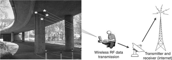
Existing commercial monitoring systems use mainly wired sensor technologies that are time consuming to install and relatively expensive. In a typical civil monitoring application a large number of sensors (i.e., more than ten) connected through long cables are used. Therefore, one of the key features desirable in monitoring large civil infrastructures as bridges is remote monitoring. Replacement of these cables with wireless systems is a longstanding dream that has become a growing reality in recent years, thanks to digital communications progress. Wireless monitoring systems, along with performance enhanced sensors based on MEMS, could poten- tially reduce these costs significantly, and would increase the field of application. An implementation of wireless AE technique sensors was proposed by Grosse et al.,30 and the basic concept is reported in Fig. 6.8. Then by using more efficient inspection methods with detailed information on the structural behaviour, maintenance costs could also be reduced.
An associated cost-cutting development is the introduction of self-powered (energy harvesting) AE systems.31 Being wireless and self-powered, the AE system could be positioned there permanently. This is in the long term a cheaper option since if the costs, for example, of a lane closure are taken into account, it becomes clear that it is cheaper to leave the equipment in place than to close the lane in order to remove it.
For these above reasons, coupling self-powered and wireless AE systems is expected to bring about a major improvement in the practical applicability of AE technology to monitor urban infrastructures.
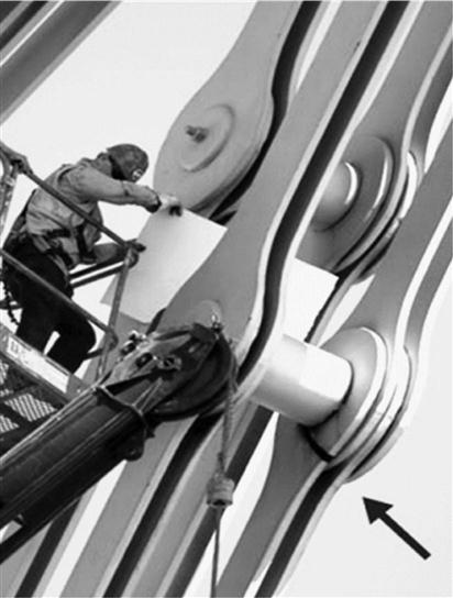
In 2009 a large crack was found in a fracture-critical element on the San Francisco–Oakland Bay Bridge by an on-site visual inspection (Fig. 6.9). An AE monitoring system was developed32 and tested, validated through laboratory testing for continuous monitoring to detect and localize crack initiation and growth in real time (Fig. 6.10).
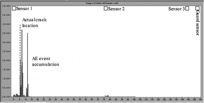
A comparison of the AE results with ultrasonic, dye penetrant and visual methods in terms of the damage detection was carried out. This study showed that the initiated fatigue crack in an eyebar under fatigue loading was successfully detected, located and monitored. In addition, by using a relatively small number of AE sensors, crack nucleation was detectable and located during the early stages utilizing a relatively small number of AE sensors. Figure 6.10 shows the location histogram recorded during the fatigue cycles of the loading and the actual crack location.
As a result of this successful demonstration of the effectiveness of the AE approach, a system consisting of 640 AE sensors connected to 16 AE Workstations was installed on the San Francisco–Oakland Bay Bridge.
In Reference 1 the AE testing was evaluated on notched full-scale hon-eycomb sandwich composite fuselage panels as a tool for NDT method for detecting crack initiation and progression, localization of the site of damage and anticipation of ultimate fracture in using redundant arrays of AE sensors. A number of panels with different damage scenarios were studied, under a combination of quasi-static hoop and longitudinal loads. Various inspections were used to assess damage progression and location, and the AE results were correlated with photogrammetric strain fields.
The locations of the events generated by new cracks at the notch tip were identified by accounting only for the high-intensity events. Post-test signal processing was applied by filtering the AE data set according to intensities that discern emissions generated primarily by new failures from that generated by other extraneous sources.
The results showed that AE techniques could accurately detect notch-tip damage initiation and track its growth to ultimate failure.
6.8 Future challenges
In spite of being a promising tool, there are still a number of challenges to be met before the successful application of AE for civil infrastructures. The main hurdles to be overcome are:
• Handling of large amount of data during testing. Due to the high sampling rate needed for data capture, a large amount of data is usually needed for a meaningful set of AE data. This is particularly important for civil infrastructures, given their long-term usage. This will encourage the scientific community to develop and implement effective analysis, fusion and management of large collection of data minimizing human intervention and interpretation.
• Reliable and effective extraction of damage sensitive data from measurements. A number of unwanted sources can produce AEs; therefore, strategies and tools for source discriminations should be in place to identify genuine failure data from spurious data.
• The effect of environmental effect should also be carefully understood and quantified on effective damage assessment.
• Automatic onset time determination for acoustic source localization. While a number of algorithms have been developed to detect TOA, a number of challenges must still be resolved. This is particularly evident for dispersive media and/or tapered structures, where mode conversion could occur. Classical time-of-flight (TOF)-based methods assume known values of AE wave velocity; however, this is inaccurate when the wave velocity changes with the propagation direction (e.g. anisotropic composite multilayered panels etc.) or with the propagation distance (e.g. tapered sections).
• Quantification damage level and prediction of durability and remaining life time. B-values and intensity analysis using severity and historic indices are promising methods; however, understanding the condition of the structure is still an on-going issue.
• Long-term performance of monitoring systems in 'hostile' environments. This is a common challenge for a variety of fields, including aerospace, marine, and so on. The performance of attached/embedded systems should be carefully monitored to avoid false alarms due to transducer failure, and adhesive bonding from real material changes.
• Long-term and power storage availability. While significant progress has been made to date on developing a reliable wireless system, the availability of long-term power for permanently installed AE systems should be addressed. Clearly, for some structures a solution would be to gather health data by employing a discrete monitoring system with limited operational life. This pushes the research community towards a unified approach whereby the energy harvesting and power storage concepts are intrinsically tied to SHM systems and should be developed and implemented simultaneously. Finally, long-term reliability of power storage and energy harvester should also be further developed.
6.9 Conclusion
In this chapter, an overview of AE for civil applications is presented. Basic principles of AE and methods for the localization of AE sources are discussed. Most of the methods discussed in this chapter assume a homogeneous and isotropic material, an assumption that is generally valid for materials used in construction. However, some examples considering non- homogeneous and non-isotropic materials are also shown. Different past and current approaches to assess the severity of flaws/cracks are reviewed. A number of applications of AE use for SHM of civil structures are described. Finally, major current and future challenges to be met for the successful application of AE for civil infrastructures are introduced.