14.3.1 Camera calibration

Camera calibration is the recovery of the intrinsic parameters of a camera. Traditionally, cameras, especially metric cameras, are calibrated in laboratories in a well-controlled environment. Laboratory calibration can be done using either a goniometer or a multicollimator (Mikhail et al., 2001). Although the camera parameters can be obtained with high precision, the calibration is rather intensive and costly. In addition, the principal distance of the calibrated cameras needs to be fixed during application, which limits the flexibility of these laboratory-calibrated cameras. More and more uses of non-metric cameras have demanded more flexible, and preferably on-site, calibration.

A general projective camera, such as the one equipped with CCD sensors, can be described using a pinhole model as (see Fig. 14.1):

$\mathit{\lambda m}=\mathit{PM}$ [14.1]

[14.1]

where m = (u, ν, 1)^T is a 2D homogenous image coordinate defined by pixels, a 3D real point is denoted by a homogenous vector M = (X, Y, Z, 1)^T, λ is a scale factor, and P is a 3 × 4 matrix called camera projective matrix, and can be described by the following relationship:

$\mathit{P}=\mathit{KR}\left[\mathit{I}\left|\mathit{t}\right)\right]$ [14.2]

[14.2]

$\mathit{K}=\left[\begin{array}{ccc}\hfill {\mathit{\alpha }}_{\mathit{x}}\hfill & \hfill \mathit{s}\hfill & \hfill {\mathit{u}}_{\mathit{o}}\hfill \\ \hfill 0\hfill & \hfill {\mathit{\alpha }}_{\mathit{y}}\hfill & \hfill {\mathit{v}}_0\hfill \\ \hfill 0\hfill & \hfill 0\hfill & \hfill 1\hfill \end{array}\right]$ [14.3]

[14.3]

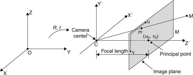
Note that α_x and α_y are the focal lengths of the camera in terms of pixel dimensions in the u and ν directions, respectively, s is the skew parameter, and u₀ and v₀ are the coordinates of the principal point in terms of pixel dimensions, R is a 3 × 3 rotation matrix representing the orientation of camera coordinate frame, I is a 3 × 3 unity matrix, and t is a 3 × 1 translation vector relating image and object coordinate system. There are a total of 11 parameters to be calibrated for a single camera, which means at least six control points have to be pre-measured (i.e., known XYZ coordinates relative to one another in an arbitrary Cartesian reference system). These camera parameters can be found by the least squares solution of Equation [14.1]. In addition, camera lens might suffer from a distortion problem that could affect the accuracy when used for videogrammetric applications. Assume an ideal image point (u, v, 1) is distorted by an unknown amount; its corresponding distorted and observed image coordinates ($\widehat{\mathit{u}},\widehat{\mathit{v}},1$ ) can be expressed as:

$\left\{{}_{\widehat{\mathit{v}}=\mathit{v}+\overline{\mathit{v}}\left({\mathit{k}}_1{\mathit{r}}^2+{\mathit{k}}_2{\mathit{r}}^4\right)+{\mathit{k}}_4\left({\mathit{r}}^2+2\overline{\mathit{v}}\right)+2{\mathit{k}}_4\overline{\mathit{u}}\overline{\mathit{v}}}^{\widehat{\mathit{u}}=\mathit{u}+\overline{\mathit{u}}\left({\mathit{k}}_1{\mathit{r}}^2+{\mathit{k}}_2{\mathit{r}}^4\right)+{\mathit{k}}_3\left({\mathit{r}}^2+2\overline{\mathit{u}}\right)+2{\mathit{k}}_4\overline{\mathit{u}}\overline{\mathit{v}}}\right)$ [14.4a]

[14.4a]

$\left\{{}_{\overline{\mathit{v}}=\mathit{v}-{\mathit{v}}_0}^{\overline{\mathit{u}}=\mathit{u}-{\mathit{u}}_0},{\mathit{r}}^2={\overline{\mathit{u}}}^2\right)+{\overline{\mathit{v}}}^2$ [14.4b, c]

[14.4b, c]

where k₁ and k₂ are coefficients of radial lens distortion, and k₃ and k₄ are coefficients of decentering lens distortion. With the selection of these additional distortion parameters, the minimum requirement for one camera calibration should increase to eight control points.

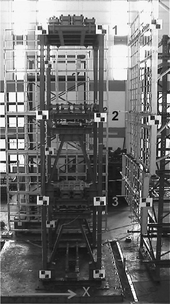
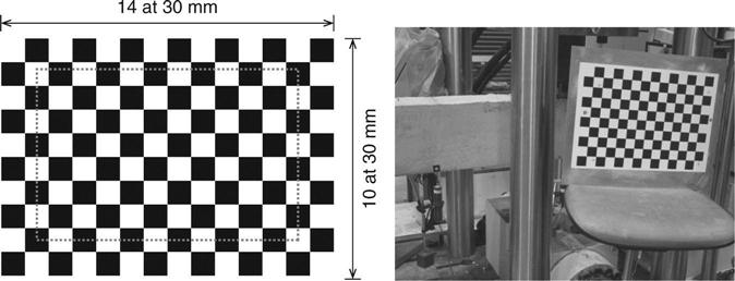
The calibration can be performed based on control targets that are spatially distributed in 3D space and not coplanar as shown in Fig. 14.2. The problem with this kind of calibration method exists in appropriate settings of cameras and targets, and tedious geometric survey of those control points. Therefore, when the measurement object or motion is not much larger, a plane-based method is considered as a more suitable way for camera calibration due to its reliability and flexibility. The plane-based camera calibration is a method between photogrammetric calibration and self-calibration that utilizes various relationships between different real plane information and corresponding image coordinates to verify all the parameters in camera projective matrices for all the views. Figure 14.3 shows one typical plane pattern for camera calibration. The corner points of black and white squares are used as control targets for the calibration.

There are several important issues related to the calibration (Kwon, 1998): (i) the calibration frame must be large enough to fully include the space of motion; (ii) the camera setting must not be altered once calibration is done; (iii) as many control points as possible should be included and spread uniformly throughout the control volume; and (iv) the calibration frame should be set properly to align the axes well in relation to the direction of motion. The camera calibration methods currently being developed in the computer vision have been moving toward more flexibility with less use of artificial control points. For example, Deutscher et al. (2000) proposed an automatic method for obtaining the approximate calibration of a camera from a single image of an unknown scene that contains three orthogonal directions (the so-called Manhattan World image).

14.3.2 Target and correspondence

Vision-based sensing is often concerned with identifying and locating pre-defined targets. These targets are used for two purposes: to provide coordinates for the point of interest, and to establish correspondence for the point of interest in an image sequence. A number of techniques can be used to locate a predefined target. These techniques depend on the type and shape of the target, whether its image is affected by perspective effects, and how much its average gray level differs from the background.

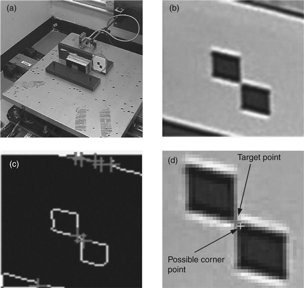
Figure 14.4 shows the identification of one common target. The algorithm includes the following tasks: (i) convert images to binary form; (ii) obtain intersections of image skeleton using image morphology techniques; (iii) filter out the outliers and determine the most-likely corner point; and (iv) use the detected point in Step (ii) as an initial guess to find the exact corner point using corner detection techniques such as the Harris corner detection method. After a target point has been identified from one image frame, it is necessary to track this target point from the subsequent images. A point matching criterion can be introduced to solve this correspondence problem. Assume that the target point is the center pixel of a square mask with r rows and c columns as shown in Fig. 14.5. A cross correlation coefficient between square mask a in Image I and square mask b in Image II can be calculated as follows:

${\mathit{k}}_{\mathit{a},\mathit{b}}=\frac{{\displaystyle \sum _{\mathit{i}}^{\mathit{r}}{\displaystyle \sum _{\mathit{j}}^{\mathit{c}}\left({\mathit{f}}_{\mathit{a}}\left(\mathit{i},\mathit{j}\right)-{\overline{\mathit{f}}}_{\mathit{a}}\right)*\left({\mathit{f}}_{\mathit{b}}\left(\mathit{i},\mathit{j}\right)-{\overline{\mathit{f}}}_{\mathit{b}}\right)}}}{\sqrt{{\displaystyle \sum _{\mathit{i}}^{\mathit{r}}{\displaystyle \sum _{\mathit{j}}^{\mathit{c}}{\left({\mathit{f}}_{\mathit{a}}\left(\mathit{i},\mathit{j}\right)-{\overline{\mathit{f}}}_{\mathit{a}}\right)}^2*{\displaystyle \sum _{\mathit{i}}^{\mathit{r}}{\displaystyle \sum _{\mathit{j}}^{\mathit{c}}{\left({\mathit{f}}_{\mathit{b}}\left(\mathit{i},\mathit{j}\right)-{\overline{\mathit{f}}}_{\mathit{b}}\right)}^2}}}}}}$ [14.5]

[14.5]

where f is the pixel gray level, $\overline{\mathit{f}}$ denotes the mean gray level of square mask, and k_a,b is the correlation coefficient that satisfies k_a,b ≤ 1. Among those candidate points, the point that gives the maximum k_a,b value is the one matching with the reference. A triangular method can be used to determine the 3D coordinates of the target point from two image points recorded by a calibrated camera.

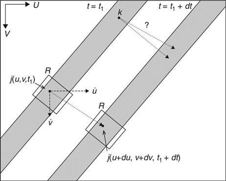
When no target is available, an approach developed in the computer vision, the optical flow technique, can be used (Jain et al., 1995). Optical flow is the velocity field resulting from an intensity change on the image plane. Figure 14.6 shows a schematic illustration of the optical flow technique. Two segments of cable images, one from time t = t₁ and the other from time t = t₁ + dt, are overlaid in the figure, where dt is a time increment. Without a specific target, it is impossible to know precisely where a point, say point k, would move to in the next time instant. Assume that the intensity of a point j(u, v, t₁) at t = t₁ is expressed as I(u, v, t₁) where u and v are the coordinates on the image plane. At t = t₁ + dt, this point moves to j(u + du, v + dv, t₁ + dt) with an intensity of I(u + du, v + dv, t₁ + dt) where du and dv are the displacement increments along u and v, respectively. These two intensities can be approximately related through Taylor series expansion as:

$\mathit{I}\left(\mathit{u}+\mathit{du},\mathit{v}+\mathit{dv},{\mathit{t}}_1+\mathit{dt}\right)\approx \mathit{I}\left(\mathit{u},\mathit{v},{\mathit{t}}_1\right)+{\mathit{I}}_{\mathit{u}}\mathit{du}+{\mathit{I}}_{\mathit{v}}\mathit{dv}+{\mathit{I}}_{\mathit{t}}\mathit{dt}$ [14.6]

[14.6]

where I_u, I_v, and I_t denote the partial derivatives of the intensity with regard to u, v, and t, respectively. Assuming the lighting on the cable segment is the same on the two images, the two intensity values can then be assumed to be the same. And we can easily derive the governing equation of pixel movement as follows:

${\mathit{I}}_{\mathit{u}}\dot{\mathit{u}}+{\mathit{I}}_{\mathit{v}}\dot{\mathit{v}}={\mathit{I}}_{\mathit{t}}$ [14.7]

[14.7]

where $\dot{\mathit{u}}$ and $\dot{\mathit{v}}$ are the velocity components of the image point j(u, v, t₁), and ${\left(\dot{\mathit{u}}\dot{\mathit{v}}\right)}^{\mathit{T}}$ is termed as the optical flow vector. Furthermore, on the assumption that there is a region of interest (ROI) R in which all points have the same constant optical flow vector, this optical flow vector should satisfy the following equation:

$\left[\begin{array}{ll}{\displaystyle \sum {\mathit{I}}_{\mathit{u}}{\mathit{I}}_{\mathit{u}}}\hfill & {\displaystyle \sum {\mathit{I}}_{\mathit{u}}{\mathit{I}}_{\mathit{v}}}\hfill \\ {\displaystyle \sum _{\mathit{R}}^{\mathit{R}}{\mathit{I}}_{\mathit{u}}{\mathit{I}}_{\mathit{v}}}\hfill & {\displaystyle \sum _{\mathit{R}}^{\mathit{R}}{\mathit{I}}_{\mathit{v}}{\mathit{I}}_{\mathit{v}}}\hfill \end{array}\right]\left\{\begin{array}{c}\hfill \dot{\mathit{u}}\hfill \\ \hfill \dot{\mathit{v}}\hfill \end{array}\right\}=-\left\{\begin{array}{c}\hfill {\displaystyle \sum {\mathit{I}}_{\mathit{u}}{\mathit{I}}_{\mathit{t}}}\hfill \\ \hfill {\displaystyle \sum _{\mathit{R}}^{\mathit{R}}{\mathit{I}}_{\mathit{u}}{\mathit{I}}_{\mathit{t}}}\hfill \end{array}\right\}$ [14.8]

[14.8]

This equation can be used to compute the optical flow vector. The direction and the magnitude of the optical flow vector then indicate the direction and the magnitude of motion for the ROI in the image plane.

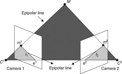
For the case of an object moving in the 3D domain, the optical flow technique can still be adopted using two or more cameras. For a two-camera image acquisition system, the epipolar geometry condition requires that two optical centers of the cameras C¹ and C², the point M, and its image projection points m¹ and m² should lie on the so-called epipolar plane as shown in Fig. 14.7. The two image points should satisfy the following equation (Hartley and Zisserman, 2003):

${\left({\mathit{m}}^1\right)}^{\mathit{T}}\mathit{F}{\mathit{m}}^2=0$ [14.9]

[14.9]

where F is defined as the fundamental matrix. This equation essentially defines a line on the second image if the image coordinates on the first image are given and vice versa. It is then possible to establish a point correspondence from the two images without the use of any target.

14.3.3 Camera movement

Most vision-based sensing techniques were developed based on the assumption that the camera was fixed on the ground. On the other hand, more and more applications in the computer vision community have demanded an investigation into the effect of camera motion, termed the ego-motion, on image understanding. The object motion recorded on an image sequence is a combined result of the actual object motion and the ego-motion. The effect of ego-motion becomes an issue of great concern for civil engineering applications. Civil infrastructures are normally large, and mounting cameras on fixed supports becomes a challenge. Several algorithms have been developed to extract the motion of a camera moving with respect to a fixed scene. These methods can be categorized either as discrete-time methods or as instantaneous-time methods (Tian et al., 1996). Simultaneous recovery of object motion and ego-motion has also been studied (Georgescu and Meer, 2002).

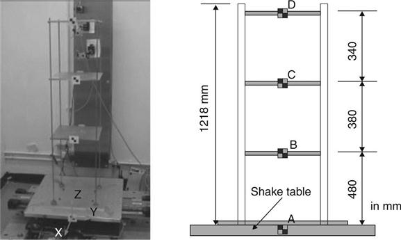
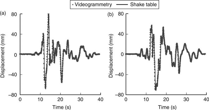
14.4.1 Small-scale building model test

In this example, the plane-based method introduced above was used to calibrate two non-metric cameras. The small-scale three-story building model was made out of aluminum with a uniform story height of 0.38 m and a total height of 1.21 m as shown in Figure 14.8. Four targets, A, B, C, and D were attached to the base and the three stories. The model was excited by the NS component (i.e. the earthquake component in the ‘North-South’ direction) of the 1940 El Centro earthquake ground displacement record and the 1995 Kobe earthquake 2D ground displacement record, respectively. Four laser linear variable differential transformers (LVDTs) were set up to measure the displacement time histories for the shake table and the three stories. Figures 14.9 and 14.10 show the two sets of results. These results indicate that image-based measurement can achieve good agreement with the LVDT measurement.

14.4.2 Large-scale steel building frame test

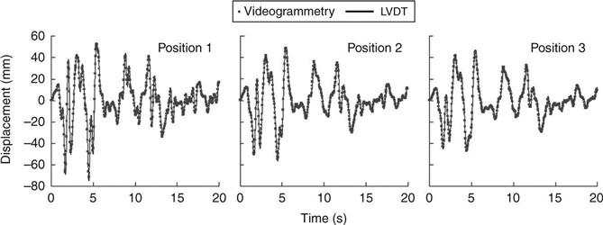
As shown in Fig. 14.2, a three-story steel building frame was mounted on a shake table in the National Center for Research on Earthquake Engineering of Taiwan. This frame was excited by the 1940 El Centro earthquake 2D ground displacement record. The frame model had dimensions of 3 m × 4 m × 12 m with three stories evenly distributed in height. Fourteen control targets were attached on and around the frame for calibrating the two cameras. Some of these targets were used as target points for the displacement measurement. All control points were carefully surveyed by a total station. The camera calibration results showed that the mean reconstruction error of all targets was around 0.5–0.8 mm, which provided an indication on the measurement error for the set-up. Figure 14.11 shows the comparison of measurement results between the image-based technique and the LVDT. It can be seen that the proposed videogrammetric technique is able to track the dynamic displacement quite accurately.

14.4.3 Wind tunnel bridge sectional model test

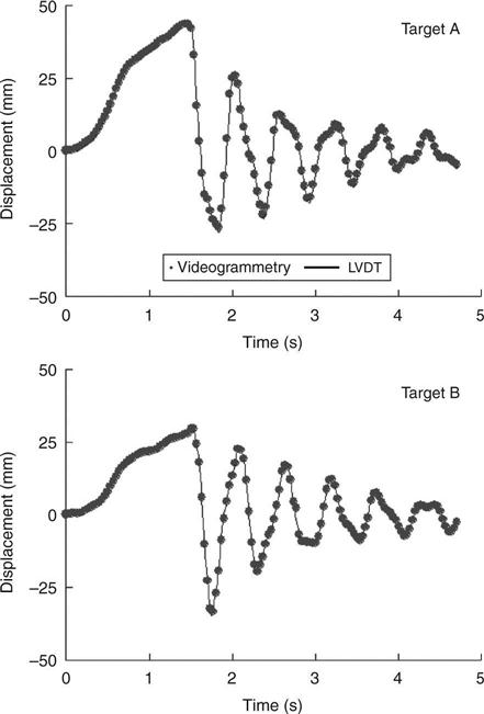
Figure 14.12 shows a wind tunnel set-up for a bridge sectional model test. The sectional model consisted of two wooden box girders connected by crossbars. The model was rigidly connected to circular rotatable shafts. The shafts were then attached to rigid rectangular bars, which were supported by four linear springs to provide the necessary stiffness for the section model. Two laser LVDTs were positioned at locations as shown in Fig. 14.12 to measure the displacement time histories during the test. Two targets were placed at locations as shown to validate the applicability of the vision-based sensing technique for such a test. The cameras were placed at about 1.2 m from the targets and the angle between the two cameras was about 30°. The focal lengths of the two cameras were both set at 15.6 mm. The model was pulled by a string and released to vibrate under a mild and steady wind condition. As the supporting rectangular bars were rigid, the readings from the laser LVDTs could be linearly scaled to the deformations at the two target locations for comparison. Figure 14.13 shows the measurement results at the two target locations. The close match between the two measured results indicates that the vision-based sensing technique is able to track the two targets quite accurately.

14.4.4 Bridge cable test

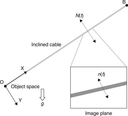
In this example, the use of the optical flow approach for measuring bridge cable vibration (in-plane motion) by monocular-vision-based sensing technique is demonstrated. Only one camera is used for the image acquisition. Assume that a bridge cable vibrates predominately along the in-plane perpendicular to chord direction as shown in Fig. 14.14. Any point on the cable can be regarded as making a 1D motion. Define the line trajectory of this point in the 3D object space and in the 2D image plane as N(t) and n(t), respectively, where t is time. For a projective camera, the mapping between the 1D motion in the 3D object space and the corresponding 1D motion in the 2D image plane can be obtained via a pinhole camera model. For a line-to-line projection, the camera matrix P becomes a 2 × 2 matrix:

$\mathbf{P}=\left[\begin{array}{cc}\hfill {\mathit{p}}_1\hfill & \hfill {\mathit{p}}_2\hfill \\ \hfill {\mathit{p}}_3\hfill & \hfill {\mathit{p}}_4\hfill \end{array}\right]$ [14.10]

[14.10]

where p_i, i = 1–4 are the camera projection coefficients. Eliminating λ in Equation [14.1] gives:

$\mathit{n}\left(\mathit{t}\right)=\left({\mathit{p}}_1\mathit{N}\left(\mathit{t}\right)+{\mathit{p}}_2\right)/\left({\mathit{p}}_3\mathit{N}\left(\mathit{t}\right)+{\mathit{p}}_4\right)$ [14.11]

[14.11]

It can be seen that the line N(t) in 3D space and the line n(t) on 2D image plane are nonlinearly correlated. Under the affine camera assumption, p₃ in the camera matrix is equal to 0. Hence, Equation [14.11] becomes:

$\mathit{n}\left(\mathit{t}\right)={\mathit{p}}_1^{\prime }\mathit{N}\left(\mathit{t}\right)+{\mathit{p}}_2^{\prime }$ [14.12]

[14.12]

where the scaling factor p′₁ = p₁ / p₄ and the initial factor p′₁ = p₁ / p₄.

It can be seen that the 1D motion in the 3D object space N(t) and its corresponding 1D motion in the 2D image plane n(t) are linearly correlated and their frequency contents would be the same. Under such conditions, it is possible to obtain the natural frequencies of stay cables from the cable image motion recorded from a single camera. The object motion N(t) can be obtained from the image motion n(t) if the scaling factor p′₁ can be determined. Setting the initial factor p′₂ = 0, the 1D motion in the object space N(t) can be obtained from the 1D motion on the image plane n (t) as:

$\mathit{N}\left(\mathit{t}\right)=\frac{\mathit{n}\left(\mathit{t}\right)}{{\mathit{p}}_1^{\prime }}$ [14.13]

[14.13]

It should be noted that the estimation of cable displacement presented above is applicable to those cables without a noticeable sag effect.

To illustrate, one cable of a small cable-stayed pedestrian bridge (see Fig. 14.15) was selected for measurement. The diameter of the cable was measured to be 40 mm. This cable was subjected to an initial deformation in the vertical plane and underwent free vibration. Two camcorders, placed at 2 and 3 m distance, respectively, were employed to measure the vibration of the cable separately. The focal lengths for both camcorders were set at 52 mm, and the ratios of the field of view to the cable-camera distance were both around 0.07 to meet the assumption of an affine camera. The two camcorders recorded the motion of the same segment on the cable so that comparison could be made. A total station was used to measure the coordinates of the two camcorders as well as the two anchorage locations of the cable. An accelerometer was also attached to the cable to obtain the cable frequencies for comparison.

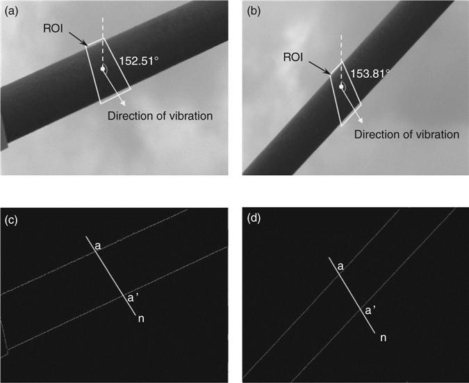
Figures 14.16a and 14.16b show one of the images captured by Camcorders 1 and 2, respectively. From the optical flow technique, the directions of the optical flow vector for the ROIs from Camcorder 1 and Camcorder 2 are shown in Figs 14.16c and 14.16d. Plate XIa (in the color section between pages 294 and 295) shows the displacement time histories of the cable segment obtained from both camcorders. It can be seen that the cable segment oscillates between − 30 and 30 mm. Plate XIb shows the power spectral densities of the two displacement time histories shown in Plate XIa. It can be seen that in the frequency range of 0 to 8 Hz, the current image-based technique can obtain three frequencies: 2.05, 3.81, and 5.84 Hz. Three frequencies can also be obtained from the accelerometer: 2.05, 3.81, and 5.76 Hz. These results indicate that the vision-based sensing technique is capable of measuring the natural frequencies of this bridge cable quite accurately.

14.4.5 Pedestrian bridge test

This test was conducted on a small-scale single-pylon pedestrian bridge. The 3D dynamic displacement of the bridge deck was measured using monocular-vision sensing technique. The planar target used for the camera calibration and the target tracking was placed at one side of the bridge deck (see Fig. 14.17). The camera was placed at about 5.2 m away from the target at about the same height, and the extrinsic parameter of the camera from the first frame indicated that the inclination angle between the Z and − Z_c axes was about 59.5°. The bridge was excited by two persons jumping on the bridge deck. A 20s image sequence was recorded for measuring the three-dimensional motion of the target. Based on the predefined world coordinate system, the displacement of the bridge deck was predominately along the X direction.

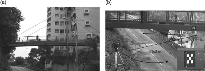
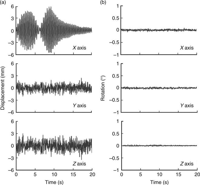
Figure 14.18a shows the measured displacement time histories along X, Y, and Z axes, respectively. It can be seen that the displacements along the X direction are larger than those along the other two directions. The first 9 s of the X displacements corresponds to the period of time when the bridge vibration was building up by the two persons continuously jumping on the deck. Beyond that the jumping was stopped and the bridge went through a free decay vibration, as shown in Fig. 14.18a. The maximum displacement amplitude along the X direction is about 6 mm. The measured displacements along the Y and the Z directions, however, do not show the built-up and the free decay behavior as seen along the X direction. These Y and Z displacements can be regarded as due more to the measurement noise than to the actual displacement of the bridge deck. The standard deviations of the displacements along the Y and the Z directions are found to be 0.76 and 1.09 mm, respectively. Figure 14.18b also shows the measured rotation angles about the three axes, which were all found to be less than 0.1°.