
Design and selection of wireless structural monitoring systems for civil infrastructures
M.B. Kane, C. Peckens and J.P. Lynch, University of Michigan, USA
Abstract:
A dichotomy exists in structural monitoring installations: those with sensors tethered to the data repository with wires, and those which use wireless communication to create a distributed network of sensors. This chapter discusses the impact of the paradigm shift from the wired monitoring systems traditionally used, to the wireless systems recently developed. This new technology is capable of achieving effective measurements on par with its predecessor, and introduces new possibilities of large-scale networks of hundreds of sensors made possible by low installation costs and scalable in-network data processing. Design and selection considerations covered in this chapter include network architecture, wireless node hardware, and distributed embedded software. Although rapidly maturing and reaching commercialization, research opportunities still exist in the fields of data and power management, which are discussed as the chapter culminates.
Key words
wireless sensors; ZigBee; sensor network; multi-hop communications; time synchronization
16.1 Introduction
Monitoring systems transfer measurement data between sensors and a data aggregator (i.e., data acquisition system) via three possible modes: conductive wires, optical fibers, and wireless radio waves. This chapter is aimed at readers familiar with traditional wired and optical monitoring systems but wishing to learn more about the design and deployment of state-of-the-art wireless sensor networks (WSNs) for structural monitoring applications. Throughout the chapter, recommendations are given that take advantage of the two key features available in wireless monitoring systems: low costs and embedded data processing. Low installation costs are made possible by wireless communication, and in-network distributed data processing is made possible by the embedded computing capabilities integrated into the hardware design of the wireless sensors.
The potential to reduce the cost of sensor installations in large, complex structures is a major driver of the growing interest in wireless sensing. An associated benefit of lower cost sensors is the possibility of deploying increasing numbers of sensors in a structure. The ability to process raw sensor data at the wireless sensor node reduces volumes of measurement data into more compressed information. This improves the system scalability, reduces power requirements, and ensures that the system communication is reliable.
This chapter will proceed as follows: the remainder of this section will summarize the motivation for the paradigm shift to wireless telemetry. Section 16.2 then provides the reader with elementary knowledge of wireless communications, including the hierarchical design model. Section 16.3 contains an overview of WSN hardware and peripherals. A selection of commercially available wireless sensors and academic prototypes is presented, but this is by no means an exclusive list and is meant only to provide the reader with the advantages and disadvantages of broad families of wireless sensors. Section 16.4 describes the firmware that is embedded in the wireless sensors and the selection criterion for key features. The chapter concludes with Section 16.5, which lays out the future commercial opportunities and research needs for the wireless monitoring field.
16.1.1 State of the practice
The advances made by the structural health monitoring (SHM) community over the past two decades will only benefit society if the value of the information provided by these systems is able to offset the costs of installation and operation of the SHM systems themselves. Presently, monitoring systems are considered cost-effective for only a select set of scenarios:1
• prior to, or during, structural retrofits,2
• following a possible overloading (e.g., after a bridge–ship impact3),
• during demolition or retrofit,4
• continuously, when long-term degradation is suspected (e.g., corrosion5),
• as needed for the performance assessment of building codes,6
• continuously, when there are concerns about the fatigue life of the structure,7 and
• during the construction of novel structural systems.8
The common attribute among all of these motivations for monitoring is that the structure’s owner or other major stakeholders can see a low-risk, short-term return-on-investment for the monitoring system. That return can be realized as reduced liability, more cost-effective maintenance decisions, or reduced construction costs.9
For example, the 2011 Los Angles Amendment Building Code §91.1613.1010 requires the installation of a limited number of accelerometers to measure strong ground motions and structural responses in areas of high seismicity. The information collected by these relatively inexpensive systems has been used for post-disaster condition assessment and improvement of seismicity models.11 In one case, inspection of accelerometer data showed that damage had occurred to a building during an earthquake. However, the location of the damage could not be identified and manual inspections of the structural connections were still necessary, costing a few hundred to a few thousand dollars for each connections.12 A reduction in per-sensor installation costs, and the introduction of innetwork data processing, both made possible with a WSN, may bring about automated condition assessment with higher spatial resolution, thereby reducing the need for costly manual inspections.
Moss and Matthews1 categorize the sensors used for SHM into three groups: those sensors that measure the application of loads to the structure (e.g., wind pressure sensors, anemometers, thermometers, and load cells); those that measure structural responses to applied load (e.g., linear variable differential transformers (LVDT), inclinometers, fiber optics, accelerometers, and strain gages); and those that directly measure structural degradation such as scour and corrosion. Transducers in these categories can vary greatly in price, from less than a dollar to over ten thousand dollars per sensor. The quintessential trade-off with cost is performance; a more expensive device will generally have a lower noise floor, better resistance to extreme environments, higher sensitivity, and a broader frequency response. Variations in these performance measures all affect the capabilities of the SHM system as a whole. The actual cost of monitoring systems has been noted to be up to $4000 per channel for strong ground motion accelerometers in buildings.6 At these prices, the broad application of SHM systems is in doubt, especially when higher sensor densities are required for improved spatial resolution of damage detection. Clearly, lower cost sensors are direly needed.
Toward achieving this goal, academia and industry alike have focused effort on reducing the cost of SHM by exploiting recent wireless communication breakthroughs. The main challenges associated with the design and deployment of a successful structural monitoring program are cost-effective data transmission, data management, and system identification (ID).9 Each of these challenges is lessened when switching to a wireless monitoring system, but new surmountable challenges arise (e.g., supplying wireless nodes with power and maintaining data quality on par with wired systems13). The development of a cost-effective, high-performance SHM architecture with wireless telemetry has applicability beyond civil structures (e.g., aircraft14 and naval vessels15,16).
16.1.2 State of the art
The idea of structural monitoring using wireless data transmission was first proposed by Straser and Kiremidgjian17 in the mid 1990s as a method to reduce the costs associated with using cables. Since then, researchers have developed a wide variety of wireless sensor prototypes aimed at reducing power requirements, extending communication ranges, and improving the efficient use of available bandwidth. Lynch and Loh18 present an extensive summary review of the developments in wireless monitoring for SHM. As the research has developed over the years, it became apparent that switching to wireless telemetry would achieve more than a cost reduction associated with the absence of extensive cabling. The embedded computing inherent in each wireless node can be used to process data in a decentralized manner, thereby reducing the computational load on the centralized server and simultaneously improving system scalability to larger nodal counts. With improved scalability comes an increased sensor density, leading to more accurate system ID and improved damage detection capabilities.
WSN for SHM can come in many flavors. Most of the research and methods presented herein consider wireless SHM as the practice of replacing wired communication between transducers and a central data aggregator with a wireless link. The wireless links most often use the industrial, scientific, and medical (ISM) radio frequency (RF) spectrum, as defined by the International Telecommunications Union (ITU) and adopted by the US Federal Communications Commission (FCC). The key benefit of using this spectrum is the ability to transmit without a license, provided local regulations are met. Within the ISM spectrum, many WSNs operate around 2.4 GHz due to high information throughput; however, 900 MHz has been used when an increase in range was required.18 Cellular data networks, i.e. the networks typically used for mobile phones, have also been used in SHM to transmit data from the small on-site data repository to an offsite server managed by the SHM system operator.19 Brownjohn et al.20 pioneered a unique form of SHM that eliminates the cabling of traditional systems, but does not transmit any response data wirelessly. Instead, a global positioning system (GPS) signal is used to synchronize the clocks of independent data acquisition systems, from which the data are retrieved periodically by manual means.
Beyond moving to a new type of telemetry, SHM using WSN has introduced other exciting opportunities, such as ad hoc communication, mobile sensors, and in-network computing, all of which increase the viability of SHM. Ad hoc communication allows the communication network to self-heal in case a wireless link fails. Additionally, sensors can be upgraded, augmented, or replaced without having to significantly restructure the network.21 In all wired SHM systems, the sensors are (semi-) permanently installed and cannot autonomously move to return better SHM results. Taking advantage of the mobile freedom associated with wireless telemetry, Zhu et al. proposed and developed an autonomous wireless robot that augments the static WSN on a bridge with mobile excitation and response data.22,23 With this technology, the special resolution of the transmissibility functions used for system ID is improved without significantly increasing the number of nodes in the network. Although wireless networks have limited communication bandwidth, compared to those that are wired, each wireless node has embedded computing (e.g., a microcontroller (MCU)) that can preprocess the data, thereby reducing the amounts of data that need to be transmitted. Not only does this in-network data processing alleviate bandwidth limitations, it can also reduce data inundation of the site’s main server. Traditional system ID algorithms, such as the eigen-system realization algorithm (ERA), stochastic subspace identification (SSI), and frequency domain decomposition (FDD), have been successfully embedded as applications in a WSN, and can be used to lessen the computational load on the server. Zimmerman et al.24–26 have embedded simulated-annealing algorithms for identifying model and state-space structural parameters using only the network’s distributed computing capability, and utilized a market-based approach for dynamic computational load balancing across the network. The key to these bandwidth optimizations is the transformation, at the wireless node, of raw time-history data to a sparser domain (e.g., the frequency domain) that is then transmitted wirelessly.
With these aforementioned advantages over wired SHM, it is no wonder that researchers and commercial interests have begun successfully deploying WSN. The large majority of the deployments have been on bridge structures, because of their accountable and transparent governmental owners. In 2005, Pakzad et al.27 measured acceleration on the Golden Gate Bridge in California using 64 MicaZ wireless sensors. A multi-hop pipelining approach was used to wirelessly deliver the data from one end of the bridge to the other, a distance that a single wireless transmission could not cover. A large-scale long-term deployment of a WSN with power harvesting was installed on the Jindo Bridge in South Korea.28 Similarly, a long-term deployment of a WSN on the New Carquinez Bridge in California was integrated with advanced data management tools implemented upon an extensive cyber-infrastructure to aid the operators in analyzing the extensive amount of data collected.19 A more complete review of successful wireless SHM installations can be found in Chapter 17.
16.2 Overview of wireless networks
The primary difference between WSNs and wired sensor networks is the medium over which the sensor data are communicated to the site’s data aggregator. In order to ensure that the greatest amount of information is sent through the network with minimal delay, certain network management practices must be established. These are especially important in a wireless network, since all nodes share a limited frequency spectrum to transmit data. This is in stark contrast to wired networks, where each node has a direct link to the data aggregator. Before considering the network as a whole, it will be helpful to first consider the communication link between two nodes, since peer-to-peer connectivity is the fundamental building block upon which the network is built.
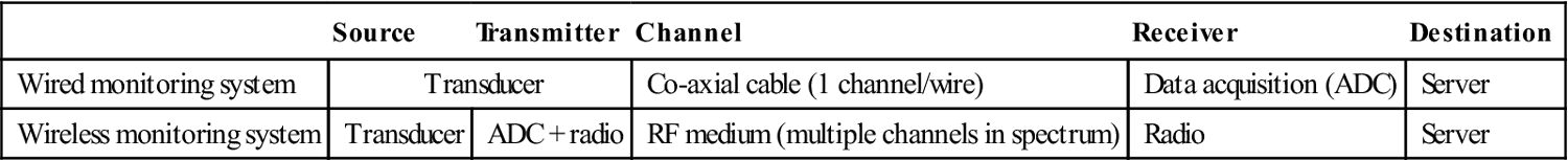
The mathematical theory of communications used to design network management practices was arguably founded by Shannon in Reference 29, in which he defines the five fundamental components of a communication link (see Table 16.1).
1. The information source generates a message and desires to communicate it to the receiver. In sensor networks, the message contains information produced by the transducer, such as acceleration, strain, or force data in the case of structural monitoring.
2. The transmitter transforms the message into a signal to be sent over the channel. An example of a transmitter in a wired strain-based SHM system is a device that converts the resistance measured across a strain gage into a voltage sent to the data acquisition system (DAQ). In a WSN, the transmitter typically converts the analog voltage produced by the transducer into a digital value, then buffers and packetizes digital measurements, modulates the digital data on a carrier frequency, and excites an antenna to transmit the data through the air.
3. The channel is the medium over which the message is transmitted. Copper cabling is most often used for wired SHM; however, fiber optics are sometimes used. Wireless systems transmit data on an RF over whatever medium is between the transmitter and receiver, whether that be air, soil, water, or building walls. The primary reason for limited communication bandwidth is signal attenuation and the introduction of natural noise occurring in the channel. In wireless networks the signal power is attenuated by the inverse square law (i.e., power ∝ (distance)− 2 )31 and noise is introduced by all sorts of electro-magnetic (EM) interference (e.g., devices emitting energy on the same frequency band, such as other networks, microwave ovens, and fluorescent lights).31
4. The receiver acts in the opposite manner to the transmitter. In a wired monitoring system, the receiver is a data acquisition system that includes an analog-to-digital converter (ADC). In a WSN, the receiver decodes the noisy and attenuated signal (i.e., message) obtained from the wireless channel and tries to recover, as closely as possible, the message that the source desired to send via the transmitter.
5. The destination is the device for which the message was intended. The ultimate destination for most messages in a monitoring system (wired and wireless) is the site’s data aggregator. However, in a WSN a message may have to ‘hop’ from one node to another if the wireless signal is not strong enough to reach from the source to the final destination.
Table 16.1
Comparison of wired and wireless communications
| Source | Transmitter | Channel | Receiver | Destination | |
| Wired monitoring system | Transducer | Co-axial cable (1 channel/wire) | Data acquisition (ADC) | Server | |
| Wireless monitoring system | Transducer | ADC + radio | RF medium (multiple channels in spectrum) | Radio | Server |
A wireless communication network is formed when a multitude of sources and destinations establish communication links between each other. Together, these links form a network that can be abstracted and described by the Open Systems Interconnection (OSI) reference model.32 The OSI reference model was created by the Organisation Internationale de Normalisation (ISO) subcommittee on OSI in 1977 as a general model to build future network specifications upon. The OSI model has subsequently been used to define the most popular network protocol architectures used for WSN (e.g., the IEEE 802.15.433 and ZigBee™ stack often used in wireless SHM networks). Wireless network standards may only define a few of the seven OSI reference model’s protocol layers (i.e., physical, data link, network, transport, presentation, and application layers) in order to remain as flexible as possible, leaving the rest up to the user to define. This division of specification responsibility for ZigBee™ networks is shown in Table 16.2 as an example.
Table 16.2
Common network stacks and development responsibility
| OSI layer | Responsible party | |||
| User application | User defined | |||
| (7) | Application layer | ZigBee | User defined | FTP or HTTP |
| (6) | Presentation layer | MIME | ||
| (5) | Session layer | SSL | ||
| (4) | Transport layer | TCP or UDP | ||
| (3) | Network layer | IPv4 or IPv6 | ||
| (2) | Data link layer | IEEE | IEEE | |
| (1) | Physical layer | 802.15.4 | 802.11 | |
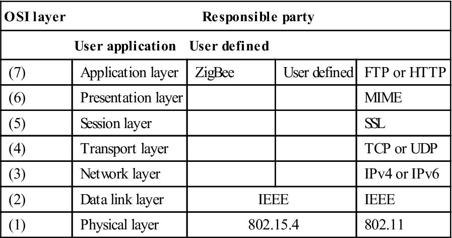
A network ‘stack’ (i.e., the software running on the nodes and server) which uses the OSI reference model comprises seven layers (i.e., groups of similar communication functions) where each layer is served by the layer below and serves the layer above. The layers start at the most fundamental physical layer and grow to become more abstract, terminating at the application layer. The seven layers and their use in some of the most popular WSN networks are described:
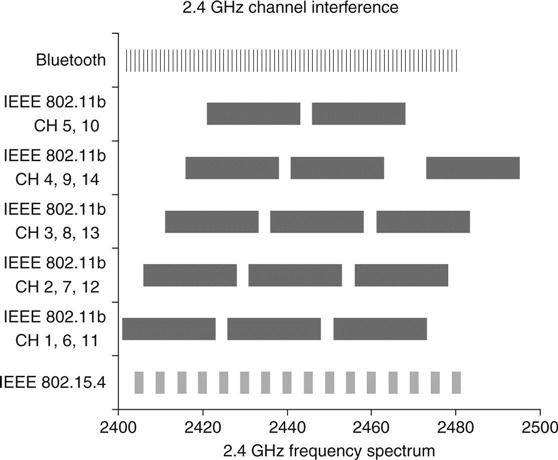
1. The physical (PHY) layer defines the method by which data are transferred over the physical media (e.g., RF spectrum of the WSN). Digital wireless communications can modulate the bits of a digital message on a carrier frequency in a variety of ways (e.g., amplitude modulation (AM), frequency modulation (FM), and phase modulation (PM)) in an attempt to make the signal less vulnerable to attenuation and noise.31 Increasing the carrier frequency (e.g., from 900 MHz to 2.4 GHz) increases the achievable data rate but decreases range especially when traveling through solid obstacles. Designers of wireless SHM networks using the popular IEEE 802.15.4 standard should note their networks will share the same physical layer (i.e., 2.4 GHz spectrum) as IEEE 802.11 wireless local area networks (WLANs) and BlueTooth™. If a WLAN is known to be present on a given channel, then the WSN should, either manually or autonomously, re-configure to use a channel in a less active segment of the shared frequency band (see Fig. 16.1).
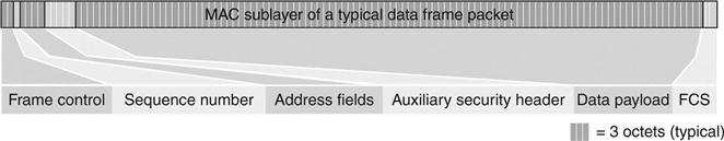
2. The data link layer establishes the link between nodes in the network using an addressing system and defines how addresses are attached to each message’s frame. In IEEE 802.15.4 networks, the data link layer comprises two sub-layers. The upper logical link control (LLC) sublayer shields upper layers of the stack from the specifics of the underlying physical layer. The lower media access control (MAC) sub-layer, whether defined by a schedule-based (e.g., time-division multiple-access (TDMA)) or contention-based protocol (e.g., clear-channel assessment (CCA)),31 establishes when nodes are allowed to transmit on the channel. Schematically, the typical IEEE 802.15.4 MAC data frame used in WSNs (Fig. 16.2) contains the source and destination address, packet sequence information, and security details, a payload of up to 102 bytes, and a check sum to ensure data integrity when received.34
3. The network layer provides routing and switching functionality. In wireless networks, the network layer is built around one of the three main topologies shown in Plate XII in the color section between pages 294 and 295: star, mesh, and hierarchical tree topologies. Star networks are often used when all nodes are within range of the central coordinator and offer high data rates; however, the failure of the coordinator or a change in the RF environment can be catastrophic. Mesh networks work especially well when the network map is not known a priori (e.g., when some nodes are mobile) or when redundant communication paths are required. Due to network management associated with mesh networks, their through-put is limited to low data rate applications. When a heterogeneous set of nodes form the WSN the hierarchical topology may be most appropriate, with the lowest-power devices serving as leaf nodes, and the higher power but more capable nodes as trunk nodes relaying messages at higher data rates, often on another frequency. While the multi-hop topologies (i.e., mesh and hierarchical) increase redundancy and range, the multiple retransmissions required to get a message from the source to the ultimate destination can significantly reduce network throughput.
4. The transport layer provides transparent and reliable data transfer to the upper protocol layers. The important wireless communication tasks of error control and failed message retransmission are handled by this layer. In WLANs, the two most popular transport layer protocols are the transmission control protocol (TCP) and user datagram protocol (UDP). The transport layer is not specifically defined by the ZigBee™ protocol and is left to the user to define if so desired.
5. The session layer controls the binding and unbinding of sessions, i.e.,brief amounts of time in which the physical layer is dedicated to data transfer between two specific nodes. Since many network stacks used in WSN are as small as possible in order to fit on a wireless sensor node’s limited memory, they do not implement a session layer. Instead, a data-transfer session comprises only a single packet, and transfer of larger amounts of data must be done in multiple packets handled by the application or by network middleware (see Section 16.4).
6. The presentation layer creates an abstracted interface to the layers below so higher-level applications may be written regardless of the type of underlying network used. The services provided by this layer include entry, display, and structuring of the data into a message.
7. The application layer should be the only layer of the OSI reference model that the user’s applications interact with and exchange network-information including network availability (e.g., determining unavailability with a time-out period). The WSN network designer is often left to define this layer; however, popular protocols such as HTTP or FTP can be implemented for this purpose.
The selection of the WSN network stack is an important design decision and should include consideration of the desired data rate, communication range, and power consumption. IEEE 802.15.4 (the foundation for ZigBee) is the preferred stack for low power and low data rate WSN.18 IEEE 802.11 (the foundation for WiFi) has been used with aggregators in large-scale WSNs where large amounts of data must be transmitted in a short period through a larger network.35 Finally, 3G and 4G cellular modems are the preferred method for transmitting data from the SHM installation site to the internet, and then to an owner’s off site repository.36
Plate XIII30 in the color section between pages 294 and 295 and Table 16.3 explains why these protocols have been used for these different purposes.
Table 16.3
Qualitative comparison of wireless standards
| OSI Layer | IEEE 802.15.4 | Bluetooth | IEEE 802.11 |
| Power consumption | Ultralow | Low | Medium |
| Battery life | Days to years | Hours to days | Minutes to hours |
| Cost and complexity | Low | Medium | High |

Source: Adapted from Reference 37.
Even after selecting the IEEE 802.15.4 physical and data link layers, there are many options available for the remaining layers that lie above in the OSI model. The three most popular are: 60LoWPAN, which implements IPv6, creating an intranet of low-power devices and is ideal when the WSN nodes will be connected to the internet (further design information can be found in Reference 3838); the precisely synchronized mesh network WirelessHART protocol was designed to bring wireless connectivity to the HART wired communication standard long used for industrial control systems (further design information can be found in Reference 39); and the low power, low data rate ZigBee protocol has found extensive use in wireless light switches, electrical meters, and other applications where data need to be communicated only intermittently.
16.3 Hardware design and selection
Structural monitoring systems are made up of three main parts: the data acquisition system (Plate XIV in the color section between pages 294 and 295 d through g), the backend data management and analytics system (Plate XIVb), and the user frontend (Plate XIVa). This chapter will focus mainly on the utilization of WSN in the context of the data acquisition system, with discussion on the effects of the data acquisition system architecture on the data management backend and user frontend. For a wireless monitoring system, the data acquisition system contains hardware called wireless sensor nodes (Plate XIVd), also sometimes called ‘motes,’ which measure physical properties (e.g., structural response to load) and transmit the measurements through a wireless network. These nodes come in many shapes and sizes, but all maintain the same principle parts.
16.3.1 Anatomy of a wireless sensor
Modern wireless sensors (Plate XIVe through g) convert a physical measure into a voltage that is then converted to a digital value, processed, and wirelessly transmitted. The sensing transducer converts the physical measure into an electrical signal that is then typically passed through a signal conditioner and into an ADC. In the node’s core (Plate XIVe), the MCU, essentially an extremely small computer, processes measurements, temporarily stores data in external memory, and then packetizes the processed data into a packet, with a destination address and other information, for transmission by a wireless transceiver. The wireless transceiver modulates the packetized data onto a carrier radio wave and transmits it over an antenna to the receiving unit or server. Optionally, wireless nodes may contain a digital-to-analog converter (DAC) that can then be used to excite the structure for active input–output system ID or for structural control.40 The whole system must be powered by either a wired power source or rechargeable batteries that can be charged using power harvesting techniques.
Low-cost, low-power MCUs have been one of the key enabling technologies for WSN. The MCU, and its embedded firmware (Plate XIVf), handles the node’s computation load but also contains a combination of other features including:
• Volatile memory (RAM) for temporary data storage (may also be on an external chip in the node)
• Non-volatile memory (EEPROM or FLASH) for storage of calibration and unit information
• Serial interface (SPI, UART, I2C) to talk to external chips (e.g., external memory, radio, ADC)
• Coprocessors for efficient calculation of fast Fourier transforms (FFTs), floating point operations, or control laws
• Timers for event counting, pulse-width modulation (PWM) generation, or watchdogs to ensure nodes do not ‘freeze’
• Internal ADC with simple signal conditioning
The selection of a MCU for a wireless sensor node is a complex task that depends upon the wireless sensor’s application. When choosing a commercial wireless sensor, it is sometimes not possible to know which MCU is used, but the node’s datasheet will typically contain abstracted specifications (e.g., speed, memory, and power consumption). Therefore, it is important for the designer of a WSN to understand the repercussion of the MCU specifications on overall WSN performance. Since wireless sensors typically run off of batteries, it is important to choose a low-power MCU with sleep modes yielding lower power consumption when a peripheral or computation is not necessary. The most common supply voltages for MCUs are 5 V and 3.3 V, but recently, lower supply voltages of 1.8 V have been growing more common since lower operating voltages generally correlate to lower power consumption. The trade-off most often associated with power consumption is computational power and speed. In other words, higher MCU speeds and computational capabilities require higher power consumption.
The lowest-power MCUs make computations using only 8-bits (i.e., numbers between 0 and 255, or − 128 to 127) at a time in a fixed-point manner. Since measurement data are stored in 16-, 32-, or 64-bit variables, many 8-bit operations are required to process each data point at the node, even for simple processing such as scaling and offset correction. Newer 16-bit MCUs are becoming more power efficient, as are 32-bit and 64-bit MCUs, yet greater power is required to operate the wider data busses. The MCU’s clock rate determines how long each primitive operation takes and can be anywhere from less than 1 MHz to greater than 500 MHz at the cost of significant power consumption. It is easiest for the user to program data processing algorithms using floating point operations. However, for efficient execution of floating point operations, the MCU should have native hardware floating point capabilities. Otherwise floating point operations must be converted to multiple fixed-point calculations. Floating point numbers stored in 32-bits are sufficient for most SHM applications, but 64-bit calculations may sometimes be necessary.
More and more MCU manufacturers are integrating additional peripherals such as ADCs, larger amounts of memory, and even wireless radio circuitry into their MCU product lines. Each of these can drive down circuit component counts and thereby reduce node costs in addition to making node design simpler. However, off-chip peripherals may still be desired if higher performance is designed (e.g., higher ADC resolution or memory size). Quality documentation, an integrated development environment (IDE), and in-system programming capabilities provided by the manufacturer or design community can further ease the job of a wireless node designer.
Important selection criteria for off-chip ADCs include resolution, speed, and power consumption. Resolutions can range from 8- to 24-bits with most structural monitoring applications using 12- or 16-bit ADCs. High sampling rates are less of an issue for structural applications with low-natural frequencies, but ultrasonic monitoring can require sampling in the MHz range. High sampling rates and resolution require greater amounts of power, and therefore should be chosen as low as possible. Other desirable features that may be available include low-power sleep modes, high data-transfer rates, and a low supply-power voltage. Additionally, a wireless node designer may want to consider ADCs with inputs capable of negative and positive voltages, integrated signal conditioning, and multiple sample-and-hold circuits with multiplexing.
Wireless radio modules (i.e., mountable transceivers) that are easily interfaced with the node’s MCU reduce the need for an RF engineer to aid in the wireless node design. These modules most often operate on the 900 MHz or 2.4 GHz ISM license-free radio frequencies using the IEEE 802.15.4 standard for the physical and data link layers. However, radios operating with other standards including IEEE 802.10 (the foundation for Bluetooth) and IEEE 802.11 (the foundation for WiFi) are available. Once again, power is a key selection criterion, which is in a trade-off with transmission range and receiver sensitivity. In fact, the power requirements of the radio are typically the greatest for the entire node. Proper antenna selection can increase communication reliability and range without increased power consumption. ‘Smart antenna’ designs that can actively control output power and signal direction are an active area of research. Well-timed sleep modes in which the receiver is shut off can save considerable power. A node designer’s job can be eased by modules with embedded firmware that automatically implement the lowest levels of the RF stack, relieving the MCU of some computation load.
16.3.2 Wireless sensor families
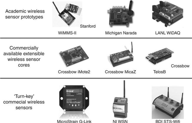
Application considerations will determine which type of wireless sensor should be used in a wireless structural monitoring system. Power consumption will be less of an issue for short-term deployments of a few days while low power consumption and power harvesting will almost certainly be required for long-term installations. The physical quantity to be measured will also affect sensor selection. While the node can be designed from scratch, it would be most advantageous to use ready-to-deploy, all-in-one commercial units if and only if available devices meet project requirements. More flexible wireless sensor modules, such as the ‘mote’ family, enable the designer to choose the desired transducer, design the power management circuitry, modify the embedded firmware, and fabricate an assembly enclosure for the specific application. If the greatest amount of flexibility is required, yet the designer wishes to not design a unit from the ground up, academic prototypes may be purchased that bring additional features such as advanced sensing (e.g., piezoelectrics41,42), feedback control,43 and the greatest amount of extensibility. In 2006, Lynch and Loh18 provided a review of available wireless sensors for structural monitoring at the time, but since technology advances so quickly, newer and more advanced wireless sensor models now exist. Regardless of the family of wireless sensors the user decides to choose from, it will be important that the datasheet of each device being considered is carefully studied. The following datasheet specifications are commonly misread and require intense scrutiny: active versus sleep power consumption along with the time anticipated to be spent active and sleep; maximum theoretical wireless data rate versus the realistic rate at which measurements can be reliably streamed; ADC resolution versus effective resolution including effects by circuit noise; transducer signal bounds, sensitivity, and signal conditioning circuitry; and wireless communication range in environments such as line-of-sight versus lightly or heavily constructed facilities. The remainder of Section 16.3.2 will compare and contrast three main families of wireless sensors currently in use (Fig. 16.3) in an effort to show readers important traits that should be broadly applicable to future generations of devices.
Commercial wireless sensors
Two classes of commercial wireless sensors exist: ready-to-deploy all-in-one units (Plate XIVe through g) and extensible wireless sensor cores (Plate XIVf though g). All-in-one wireless nodes, such as those found in the MicroStrain G/V-Link line,44 Bridge Diagnostics Inc. (BDI) STS-WiFi – Wireless Structural Testing Systems,45 National Instrument (NI) WSN line,46 the Ohm zSeries,47 and WirelessHART products by companies like Siemens,48 are robust easily deployed ‘turn-key’ solutions to wireless monitoring. Each self-contained unit includes a power source, transducer, signal conditioning circuitry, antenna, wireless radio, and computational core. The more popular units have acquired a large user base whose collective experience can be leveraged. In order to maintain an easy-to-use system, many features such as maximum sampling/data rate, in-network data processing, power harvesting capabilities, power management, design flexibility, and multi-hop capabilities are limited. These shortcomings are offset by their ease of use for inexperienced users, and by the large user base whose collective experience can be leveraged by a novice user.
When the user has specific design requirements not met by commercial turn-key solutions, commercially available wireless sensor cores (Plate XIVf though g in colour section between pages 294 and 295) in colour section between pages 294 and 295 can be used to ‘jump-start’ development of the entire sensor node. These units typically do not include protective housings, transducers, or power management circuitry; as such, peripherals must be designed or selected to bring this functionality. The ‘mote’ line of devices originating from Berkeley and manufactured by companies such as Intel, Crossbow, and MEMSIC provide the user more flexibility through an open source hardware and software design. The model in this line that has seen the most extensive use in the structural monitoring field is the iMote2,49 due to its embedded operating system (OS) specifically designed for WSNs, its extensibility through the use of daughter boards (e.g., the SHM-A boards50 with onboard accelerometer and controllable signal conditioning), and its significant computational capabilities. In the developing field of wireless SHM, commercial units are not always available for immediate purchase to meet a project’s needs. As such, the academic community and commercial sector have developed custom nodes, bringing previously unavailable features to the field.
Academic prototypes
Researchers in academia are interested in pushing the vanguard of WSN and have developed nodes with unique features not found in commercial wireless sensors at the time of their development. The costs of working with cutting edge academic prototypes are the smaller user base, required programming skills, and equipment needed for assembly and debugging. The WiMMS sensor family developed at Stanford in the late 1990s was one of the earliest wireless sensor families for SHM. WiMMS led to the development of the Narada at the University of Michigan. The Narada was the first wireless node for civil engineering applications with wireless feedback control capabilities in the original design. Both the WiMMS Sensor and the Narada featured swappable radio modules so that range, data rate, and power consumption could be tailored to the field application at hand. The wireless node developed by Bennet et al.51 was designed to be embedded into flexible asphalt to measure strain and temperature. Mitchell et al.52 proposed a wireless node with two wireless transceivers; one to talk to low-power nodes in each cluster and the other transceiver to communicate over long distances with other clusters. The WiDAQ developed at Los Alamos National Lab.53 features a unique daughter board capable of measuring the impedance of seven piezo-electric sensors per node. Recently developed at the University of Michigan, the Martlet wireless node features a dual core design that allows for real-time data processing or feedback control algorithms to run on a dedicated coprocessor with access to the internal ADC and DAC. This coprocessor leaves the main processor to handle such tasks as collaboration with other nodes. Each of these prototypes has brought something new to the field of wireless SHM, features that will likely be seen in future commercial products. Academic prototypes are similar to commercial devices, e.g. use of the IEEE 802.15.4 communication standard and 16-bit or greater ADCs. The prototype units introduced features such as feedback control, novel transducers, and dual core computations that may eventually find their way into commercial units, as was seen with corrosion sensing.54
16.3.3 Wireless sensor peripherals
Besides the node core (Plate XIVf, see colour section between pages 294 and 295), the designer or user of a wireless sensing node needs to consider attached peripherals such as transducers, signal conditioners, and energy harvesters.
Transducers
Transducers convert the physical measurand into an electrical signal that can then be converted to a digital signal. This is true for wired or WSN; as such, WSN can measure the same phenomenon as their wired counterparts, albeit sometimes in a different way as to minimize power consumption. For example, when measuring acceleration, microelectromechanical systems (MEMS) accelerometers are most often used for WSN due to their small size, low cost, and low power requirements. Displacements can be measured with LVDT or potentiometric displacement transducers (e.g., string potentiometers and axial potentiometers). Low power integrated circuits (IC) exist for measuring temperature, humidity, and light levels, often with their own signal conditioning and ADCs. Other transducers that can be interfaced with certain wireless sensors are wind vanes, anemometers, piezoelectrics, strain gages, and proximity detectors. The wide range of low-cost transducers that can be integrated with wireless sensors has led to even greater interest in wireless monitoring systems.
Signal conditioners
The theory behind signal conditioning does not change when using wireless sensors, but new practical considerations arise including power consumption, usable voltage levels, design complexity, and circuit size. Depending upon the type of transducer used, various types of signal conditioning will be required before analog-to-digital conversion. Many transducers now available on the market (e.g., MEMs accelerometers and IC temperature sensors) contain much of the analog signal conditioning required, and output a signal compatible with the most popular ADCs. Even if a transducer such as an accelerometer could be directly integrated, signal conditioning for amplification and anti-alias filtering may be desired and used. If using an older transducer or a newer one without integrated signal conditioning (e.g., metal foil strain gauges), analog circuitry will be required to convert the signal produced by the transducer into a low-noise voltage signal that is within the bounds of the ADC (most commonly 0–3.3 V or 0–5 V). Since wireless sensors are often designed to be as small as possible, the amount of space taken up by signal conditioning on the printed circuit board (PCB) should be minimized. Large analog signal conditioning circuits can often be replaced or minimized by using digital signal processing techniques, such as over sampling, or by using mixed signal ICs (i.e., ICs that process both analog and digital signals) such as the QuickFilter Technologies QF4A51255 ADC with programmable gain amplifiers, and programmable analog and digital filters. This IC was successfully used on the ‘SHM-H sensor board’,56 a peripheral board designed for use with the iMote2, with the capability to measure accelerations with high sensitivity. Less sophisticated boards, but with similar intent, have been created for interfacing strain gages with the MICA Mote,57 and strain gages and accelerometers with the Tmote Sky wireless sensor core.58 The designer of a wireless SHM system can simplify the selection process by choosing a commercial wireless node with integrated signal conditioning or can meet their application requirements by designing custom signal conditioning.
Energy management and harvesters
One of the fundamental advantages of WSNs is the absence of wires that transmit signals throughout the network. However, the ‘last wire’ (i.e., the power supply wire) to each sensor is the most difficult to do away with. In addition to designing a low-power node core, judicious selection of energy harvesters and batteries can extend the uptime of the node, or enable longer sampling periods. The estimates provided in Table 16.4 show general usage scenarios and limitations of commercial energy harvesters and battery chemistries. It should be noted that manufacturers typically specify energy densities with respect to a typical load current and environmental temperature. Large loads and winter temperatures can significantly decrease battery energy capacity.
Table 16.4
Energy densities of common WSN power sources
| Energy harvesters | Power density | Battery chemistry | Volumetric density (W Hr/L) |
| Solar (outdoors) | 15 mW/cm2 (sunny) | Alkaline-MnO2* | 347 |
| 0.15 mW/cm2 (cloudy) | Sealed lead acid | 90 | |
| Solar (indoors) | 0.006 mW/cm2 (ambient light) | NiCd | 80–105 |
| 0.57 mW/cm2 (task light) | NiMH | 175 | |
| Vibrations | 0.01–0.1 mW/cm3 | Li-ion | 200 |
| Acoustic noise | 3E-6 mW/cm2 at 75 dB 9.6 mW/cm2 at 100 dB |
Li-polymer | 300–415 |
| Applied RF | 2–8 mW61 |
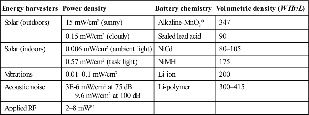
Source: Adapted from Reference 65.
Aiming to further increase the availability of energy, the research community is pushing the frontiers in two areas: power efficiency and power harvesting. Wireless node energy efficiency can be improved by selecting low-voltage components, selecting components with sleep or low-power modes, and implementing autonomous power switching of high power components (e.g., transducers). Regardless of energy efficiency, long-term deployments of WSNs will require the nodes to be recharged. Since manual replacement of batteries is expensive, the implementation of an energy harvesting system that can power a node directly or can be used to charge rechargeable batteries is preferred. Long-term field deployments of structural monitoring WSN have successfully scavenged power from vibration,59 wind,28 light (e.g., solar),36 and ambient60 or applied61 EM energy (i.e., RF). Commercial WSN vendors are beginning to market integrated energy harvesting, related products, and consulting services centered on energy management in WSN.62,63 If the WSN designer must design a custom energy harvesting solution, reference texts such as Beeby and White’s Energy Harvest for Autonomous Systems64 provide details on each mode of energy harvesting and design guidelines. By using energy efficient wireless sensors and an appropriately designed energy harvesting system, WSN can be deployed maintenance free for years.
16.4 Wireless sensor network software
There are two types of software running in wireless SHM deployments: the embedded firmware running on the wireless nodes and the software running on the server handling data presentation, processing, and archiving. This section will focus on the embedded firmware because the server-side software for wireless SHM is not much different from the counterpart for wired SHM. Embedded firmware designs can be broken down into three layers (Plate XIVg, see colour section between pages 294 and 295): the OS, middleware, and application software. These layers sit on top of the node hardware. Ideally, these layers should be independent of each other, with well-defined interface abstractions. Delineating embedded firmware in this manner has the benefit of greater amounts of code reuse, reduced development time, and decreased code maintenance costs.
16.4.1 Operating systems (OS)
The software that makes up the OS on a wireless sensor provides system management features and hardware interfaces to the upper middleware and application layers. It should be noted that the OS on a wireless node is significantly different from the OS on a consumer PC (e.g., Windows, MacOS, and Linux) due to the limited memory and computational capability on each node. The design or selection of the OS task scheduler, the software that determines when tasks are executed based on priority and timing, requires careful consideration. Since only one task can run on the processor at any given instant, the OS must be able to preempt tasks (i.e., interrupt a lower priority task to allow a higher priority task to complete) as quickly as possible by moving the current state of the preempted task into temporary memory and allocate resources for the preempting task. This feature allows an MCU to execute higher priority applications quicker in the middle of longer lower priority applications instead of having to wait for the first application to complete. However, task preemption can lead to system failures such as deadlock and task priority inversion. The former causes the processor to ‘freeze’ and can be mitigated by the strategies out-lined in Reference 66. The latter famously led to a failure of the NASA Mars Pathfinder spacecraft; fortunately, the error was discovered and fixed through a remote system upgrade.67
A robust task scheduler and the ability to perform remote system upgrades are just two of many features an embedded OS should contain. The OS should be as memory efficient as possible, since MCUs typically used in the design of wireless sensor nodes have limited memory compared to larger computing systems, such as PCs. Just as in hardware design, the software design must always consider power consumption. The processor should go into a low-power idle or sleep state after all tasks in the queue have completed and wake again when an interrupt occurs. The OS is often selected, and not designed, by the designer of the WSN. As such, the OS should be well documented and easy for the WSN designer to implement and/or develop the middleware and application layers. Besides a well-documented application programming interface (API), firmware development time will be shortened if the OS has hardware abstraction layers (HAL) for a wide variety of target processors, a strong community user base, reliable professional support, and the ability to write applications in a popular programming language (e.g., C/C++).
The ubiquity of embedded systems has led to the development of a wide range of embedded OSs. Since nearly instantaneous response to external events such as measurement sampling and radio transmissions are critical for wireless sensors, real-time operating systems (RTOS) have become popular for wireless sensors. An RTOS can guarantee certain capabilities within specified time constraints and should autonomously handle common system failures. FreeRTOS68 and the Micrium RTOS69 are open source RTOS that are available for free, allow the user to modify the source code, and have become popular for WSN. A commercial RTOS, such as Keil RTX70 for ARM processors and Wind River VxWorks71 developed by Intel, is extensively used in industry and provides professional support and a richer and more robust feature set. All of these embedded RTOSs are multi-threaded. While not considered an RTOS, TinyOS72 was developed specifically for WSN and is uniquely programmed using the nesC programming language, a derivative of C. Extra care must be taken when using a non-RTOS to ensure data collection is synchronized across the network and time-critical tasks (e.g., interrupts associated with feedback control for structural excitation) are executed with minimum jitter (i.e., small amounts of delay from when the task should have been executed to when it is actually executed). These issues have been addressed with a well-defined middleware73 in the iMote 2 sensors running TinyOS.28,50,74 Unfortunately, TinyOS is not multi-threaded, which is another limitation. The complexity, expense, and memory requirements associated with an OS are not always required, in which case a simple interrupt-based state machine along with a HAL can be custom developed. This strategy has been successfully employed on the Narada wireless sensor with a low-power 8-bit MCU and only 128 kB of external memory75 compared to the 32-bit processor on the iMote 2.0 with 64 MB of memory running TinyOS.76 A state-machine strategy can also be properly designed with interrupts so that the embedded firmware is effectively multi-threaded, yet still capable of real-time operation.
16.4.2 Middleware
Middleware is a software link between the OS and the application layer. It is intended to simplify the job of the application designer and to provide a wide variety of functionality. Wireless boot loaders are desirable because they allow remote firmware upgrades to the WSN, and can even allow software ‘agents’ to be dynamically distributed throughout.77,78 Since the IEEE 802.15.4 wireless transmission protocol (see Section 16.2) has no prescribed network layer for handling packet failure, middleware is required to correct these failures in the most efficient way, based on the WSN topology. As has been common to all aspects of WSN discussed in this chapter, middleware can improve energy efficiency, by scheduling the use of lowpower ‘sleep modes’ and duty cycling the radio receiver as discussed in Section 16.2 for TDMA wireless protocols. Additional energy can be saved by reducing the number of bits wirelessly transmitted by compressing the data to be sent using a lossless compression algorithm.79 Although structural monitoring WSN are relatively static, a method should still exist for new units to be added to the network, or existing units upgraded. Novel techniques for resource allocation include: adaptive fidelity algorithms, in which nodes are near an ‘important event’ sample with greater resolution than those far away;80 and dynamic allocation of computation resources using a buyer/seller framework.81
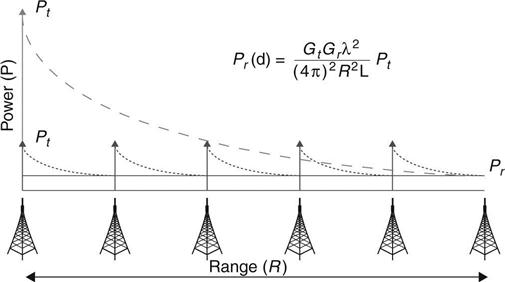
Message routing is an important middleware feature because it determines the reliability and efficiency of communications. Message routing in single-hop and multi-hop network architectures is shown in Plate XII. A multi-hop strategy, i.e., one in which the radio output power is reduced so the signal reaches only the closest node in a path to the destination, can be employed to minimize each node’s transmission power. The area under the curves in Figure 16.4 are analogous to the amount of power required to transmit over the distance shown for the single-hop configuration (dashed) and multi-hop (dotted). If n transmissions are used to cover a range R, then the reduction in total transmission power is proportional to R2/n. However, in practice, choosing the correct transmission power, if selectable at all, is a difficult task to accomplish reliably. Additionally, the power saving advantage needs to balance the increased latency associated with each ‘hop’ the message makes and the exponential decrease in reliability with respect to the number of ‘hops,’ which would increase power consumption due to many re-transmissions.
Time synchronization of the data collected by all the nodes in the WSN is an inherent challenge with wireless sensors, and is best achieved with effective middleware. In effect, each node maintains its own clock. This is in stark contrast to wired monitoring systems, where the data sampling for all sensors is triggered by the same clock channel. The presence of multiple clocks brings a unique challenge to WSN: a means to synchronize all of the nodal clocks such that an agreement on a common time basis is necessary. De-synchronization can occur on the network level due to network latency and on the hardware level due to gradual drifts of a node’s clock commonly provided by a low-cost crystal. Clock drift can be reduced by using a more expensive high quality crystal or a thermally corrected crystal that draws additional power. If no ‘hops’ are required to transmit from the network coordinator to all the nodes, a simple beacon can be used to synchronize the network to within 30 μs.82 Although synchronized, all the nodes in the network are delayed by an unknown amount from the coordinator’s timing due to radio latency on the order of 10 ms. Multi-hop mesh networks require a more complex strategy such as the flooding time synchronization protocol83 that quantifies the stochastic delay in each link of the WSN.
The most extensive middle package for SHM was developed by Nagayama, et al.73 for the iMote2 running TinyOS, and includes features such as reliable data transfer, network data aggregation, and sensor synchronization. All of the middleware solutions deployed should share a common application interface so that the application design can effectively utilize the provided features.
16.4.3 Application software
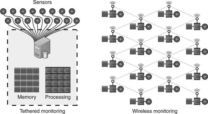
The application software embedded in the WSN is significantly different from the applications that run on a typical PC. While the available computational and memory resources might be equivalent to a PC, they are distributed across all the nodes in the network, as schematically shown in Fig. 16.5; therefore, the applications must also be distributed. Embedded applications must be efficient in terms of processor cycles, memory, and energy. Often, only a single application runs on each node due to limited local resources, while a multitude of different applications run simultaneously across the WSN. The ultimate goal of WSN applications is similar to those for wired structural monitoring systems (e.g., data management, damage detection, system ID, and even structural control). The local data processing at the node is a major paradigm shift from wired sensor networks. Important considerations for application designers include accuracy, speed, power efficiency, wireless bandwidth usage, and end-user usability.
In many structural monitoring systems, large amounts of data are collected, but only key characteristics are needed by the user. This disparity necessitates automated methods for data processing and management. For wireless impedance-based SHM the time-history data are converted to the more sparse frequency domain, which is then transferred to the site repository for future processing and analysis.53 Since the ability to compress data by domain transformations is not always possible, the data repository can direct the method by which the WSN relays the data in real-time depending on whether raw or pre-processed data is required.84
When the goal of a wireless SHM installation is damage detection, the analysis can take place autonomously, relaying only the network’s prognosis (damage versus undamaged). Automated wireless structural damage detection was first proposed by Straser and Kiremidjian, who used the Arias intensity computed at each node using local acceleration data as an indirect method to detect the energy dissipated as a component in the structure is damaged during an earthquake.17 Developed for automated damage detection application to situations other than earthquakes, ARX (autoregressive with exogenous input) models have been embedded in a WSN and the magnitude of the residual of the coefficients for nominal can be used to identify the presence of damage.85 Instead of using global vibration characteristics to detect damage in concrete structures, displacement measurements can be autonomously compared to embedded damage index models to provide estimates of local structural damage.86
An entire model of the system can be computed from vibration data using a combination of in-network computing and server-side computing. One realization use a node’s local response data to compute Markov parameters, which are then sent to the base station using significantly less bandwidth than would be required to send raw data. The Markov parameters are then input into an ERA.87 The algorithm successfully identified system parameters of an auditorium balcony using less wireless bandwidth than other strategies. These examples show that many traditional damage detection and system ID algorithms can be distributed across the computational capabilities of the nodes in the wireless network, thus increasing scalability compared to wired systems with central data processing centers.
The lessons learned from developing wireless structural monitoring systems have been extended to wireless feedback control systems. Structural control was first proposed in 1972, but has seen only limited use due to installation costs and reliability concerns.88 Augmenting these initial control systems with wireless telecommunications has been shown to lead to improved performance over completely decentralized systems, without the added cost of cabling associated with centralized controllers. Due to bandwidth limitations and latency associated with wireless communication, novel distributed control algorithms were developed that utilize the embedded computing available at each node and communicate with other nodes as little as possible.
Wireless control networks are well suited for large systems with many actuators and sensors such as semi-active control, i.e. actuation involves changing stiffness and damping properties of structural elements instead of actively applying a force. Initial research on wireless semi-active control systems considered full measurement feedback at slow sampling rates or fully decentralized control at high sampling rates.40 Building on existing optimal control theory, the sub-optimal clip-linear quadratic regulator has been an extensive topic of research, along with decentralization of the associated state estimator. One method to strategically utilize wireless bandwidth and achieve performance near that of full state feedback is to use the error between two parallel estimators on each node and request asynchronous measurement updates from other nodes in the network when the error reaches a threshold.89 The robust H-∞ control law can be applicable by homotopically transforming the feedback matrix to yield sparsity aligned with the sensor sub-networks.90 In this way, the advantage of feedback is achieved by communicating feedback data on different, non-interfering, wireless channels for each sub-network. Less traditional control techniques, but well-fitting to agent-based wireless networks, are the class of game-theory inspired actuator resource allocation algorithms. These have been experimental validated with large-scale structural-control experiments91 and can account for the inherent non-linear characteristics of semi-active control devices, a feature not present in clipped-optimal controllers.92 Most recently, a wireless control and monitoring system has been developed that unifies structural monitoring with feedback semi-active vibration control with a graphical interface for end users93 for maintenance and management.
Researchers are continuing to develop distributed algorithms for WSN that are inspired by, but different from, those found in parallel supercomputers due to the significant communication latency in wireless networks. Well-developed applications interfaced with the appropriate middleware, OS, and hardware yield a WSN that can perform as well as a comparable wired monitoring system with new features, decreased costs, and reduced installation time.
16.5 Conclusion and future trends
Wireless structural monitoring solutions are rapidly maturing. Early research and development efforts, mainly in hardware development, focused on overcoming the challenge of reliably deploying WSN on structures. These technologies have been tested and deployed in the field on buildings,94–96 bridges,28,97,98 and wind turbines.99 The early efforts paid off and have led to commercial ‘turn-key’ solutions for SHM for a limited, yet important, set of applications.
More novel systems require the application of the principles covered in this chapter to design, select, and develop a custom WSN hardware, software, and network. A significant portion of this chapter covered key options and criteria for designing or selecting the network architecture, wireless hardware, and embedded software. Single and multi-hop networks were presented as the main network architectures that supported signals on a variety of different frequencies in the RF spectrum using any number of popular wireless standards. It was shown that the embedded firmware will consist of an OS (or a simple custom solution), middleware to aid with data handling and management, and application software to present meaningful data to the network operator. The development of wireless hardware will also consist of a transducer to measure the desired structural response with appropriate signal conditioning and power management circuitry. This design process can be jumpstarted by using a commercial wireless module. While accuracy, usability, and cost play an important role, the power consumption and data handling will make or break the final design.
Currently, WSN are limited by their effective over-the-air data rates and their strong dependency on batteries. Current and future research efforts aim to exploit the in-network data processing capabilities of WSN to make them even more attractive (i.e., more scalable and power efficient). When considered as an aggregate, the limited computation capabilities of each node are a significant computational resource and can be used to autonomously execute sensor fault detection,100 data compression,101 model updating,24 system ID,87 and damage detection.102 Over the past two decades, transistor density, and thereby computation speed and efficiency, has increased at an exponential rate, while battery energy density has hardly increased linearly.103 As such, development of more efficient energy harvesting systems is a prime area of needed research. Innovative researchers have been able to harvest energy through non-resonant vibration (e.g., traffic)104 and optimally harvest energy in a distributed manner.105
With today’s relatively high rate at which data can be processed, feedback control (e.g., using semi-active dampers) and active sensing (e.g., PZT and ultrasonics) are exciting extensions to WSN. In order for all of the developments outlined in this chapter to be used commercially, ‘softer’ research efforts will have to focus on ease of use of WSN and how to make the advantages of WSN so apparent that the paradigm will shift away from wired sensing and to ubiquitous wireless structural monitoring systems.
16.6 Acknowledgments
The authors of this chapter would like to acknowledge the generous support provided by the National Science Foundation (NSF) through grant numbers CCF-0910765 and CMMI-0846256. The authors would also like to gratefully acknowledge the generous support offered by the US Department of Commerce, National Institute of Standards and Technology (NIST) Technology Innovation Program (TIP) under Cooperative Agreement 70NANB9H9008. This work was supported in part by the US Office of Naval Research (Contracts N00014–05–1-0596 and N00014–09-C0103). Finally, the writing of this chapter was partially supported by the National Research Foundation of Korea Grant funded by the Korean Government (MEST) (NRF-2011–220-D00105(2011068.0)).