
This text provides fundamental and practical technical information on smart antennas and Code Division Multiple Access (CDMA), two technologies that will play a major role in the future of wireless telecommunications. The information presented here is targeted at engineering professionals and wireless practitioners and is also suitable for graduate level course work.
In the past, wireless systems were deployed using fixed antenna systems, with antenna patterns that were carefully engineered to achieve desired coverage characteristics, but that could not change to react dynamically to changing traffic requirements. Smart antennas are a new technology for wireless systems that use a fixed set of antenna elements in an array. The signals from these antenna elements are combined to form a movable beam pattern that can be steered, using either digital signal processing, or RF hardware, to a desired direction that tracks mobile units as they move. This allows the smart antenna system to focus Radio Frequency (RF) resources on a particular subscriber, while minimizing the impact of noise, interference, and other effects that can degrade signal quality.
Code Division Multiple Access (CDMA) is a new wireless technology that allows multiple radio subscribers to share the same frequency band at the same time by assigning each user a unique code. The technology makes very efficient use of limited spectral resources and allows robust communication over time-varying radio channels. Both smart antenna technology and CDMA promise to revolutionize the field of wireless communications.
To gain a historic perspective, it is worth noting that land mobile radio was introduced as early as the 1920s to provide two-way communications to automobiles. These radio systems evolved into a number of specialized services and offered paging, dispatch, and two-way voice and data communications to mobile users. In the early 1980s, analog cellular radio systems, including the Advanced Mobile Phone System (AMPS) in the United States, the Total Access Communications System (TACS) in Europe, and the Japanese TACS System (JTACS) in Japan, were deployed, bringing untethered wireless voice access to the Public Switched Telephone Network (PSTN). In the mid-1990s, digital cellular and Personal Communications Services evolved to provide universal coverage to users, using lightweight, low power, portable subscriber handsets with the clarity of digital voice and enhanced features and services such as digital messaging and caller ID.
The recent explosion of Wireless Local Loop (WLL) in emerging countries has generated tremendous interest in adaptive antennas to provide rapid, inexpensive wireless infrastructure in emerging countries and to allow Competitive Local Exchange Carriers (CLECs) to compete in new markets. Emerging WLL systems which make use of CDMA and adaptive antenna technology have been developed to provide enhanced range, reliability, and capacity.
Recently deployed digital cellular and Personal Communications Systems will be complemented shortly by new systems that combine the clarity and capacity of digital voice systems with high rate data services, allowing video delivery, high speed Internet access, and broadband data services. Smart antennas and CDMA are critical enabling technologies that will allow the efficient use of the radio spectrum needed to provide high mobility in dense traffic areas, as well as broadband wireless access.
The concept behind cellular radio is that a finite spectrum, or bandwidth, allocation is made available throughout a geographical area by dividing the region into a number of smaller cells, as illustrated in Figure 1-1. In traditional analog cellular systems, each cell uses a portion of the spectrum. Cells which are sufficiently far apart can reuse the same spectrum resources [Rap96a]. Modern CDMA systems, as we show later in this chapter, also reuse spectral resources from one cell to the next, but in a somewhat different manner.

Figure 1-1. Cellular systems provide service by dividing a coverage region into cells. Each cell is served by a base station. Large Macrocells can have radii of several kilometers. Microcells, with ranges of hundreds of meters to a kilometer, provide service to dense, high-capacity areas. Picocells are used to provide spot coverage indoors and in high-traffic-density pedestrian areas.
The user communicates with the base station in each cell through a set of logical channels which are used for paging, access, and traffic. A channel is allocated to a subscriber when it is active in a cell and is released when the portable unit terminates the call or hands-off to another cell.
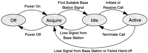
When a mobile unit is engaged in transmitting or receiving voice signals, data, or fax information, the unit is active. A mobile unit which is prepared to receive or place a call, but is not actively transmitting or receiving, is idle, as shown in Figure 1-2.
The first cellular radio systems had cell radii of several kilometers. These systems, which primarily served users in vehicles, are referred to as macro-cellular systems. Over time, as market penetration increases, the number of users in a given area which must be supported by the system increases. The number of subscribers that can be supported in an area is limited by the spectrum available and the air interface technology. To support more capacity, the power of each base station is lowered, and finite spectrum resources are reused more frequently over a geographic area. This is accomplished using very small cells, or microcells, with closely spaced base stations. In general, systems with smaller cells and densely spaced base stations have higher capacity. More recently, PCS systems have emerged with cells as small as a few hundred meters, or even small enough to cover a portion of a single floor of an office building using picocells.
While microcell systems offer enhanced capacity, they do so at the expense of high infrastructure costs, since many more base stations are required. Microcell systems can also present difficulties for high speed users that hand-off rapidly from one cell to another. To exploit the benefits of both types of systems, multi-tier systems use a combination of macrocells to serve high speed subscribers, with microcells to support high capacity areas [Rap96a].
In wireless communication systems, the radio link from the base station transmitter to the portable receiver is the forward link or downlink. The link in which the portable unit is the transmitter and the base station is the receiver is called the reverse link or uplink. Typically, the forward and reverse channels are divided into different types of channels. Control and access channels are used to set up calls and handle other control functions for idle units. The traffic channels are used to carry voice and data information. These channels are illustrated in Figure 1-3. In many systems, the uplink and downlink use channels which are separated in frequency. This technique is called Frequency Division Duplex (FDD). Other systems use the same frequency channel for both the uplink and the downlink, allowing the uplink to use the frequency slot during one time period and the downlink to use the frequency slot during the next time period. This method is called Time Division Duplex (TDD). These concepts are illustrated in Figure 1-4.
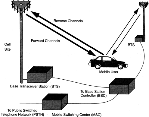
Figure 1-3. There are two main types of forward channels. Control and access channels are used to set up calls and provide security and management functions. Traffic channels are used to carry voice traffic. The reverse channels are also divided into access channels and traffic channels. In some systems, the Base Station Controller (BSC) may be integrated directly into the cell site. In other systems, as shown here, the Base Transceiver Stations (BTSs) are connected to a Base Station Controller.
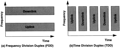
Figure 1-4. Frequency and Time Division Duplex strategies. In FDD systems, since the transmitter and receiver are simultaneously active, they must be widely separated in frequency or highly selective filters must be used to protect a subscriber unit’s receiver from its own transmissions. When a limited bandwidth is available, TDD systems are attractive because the subscriber is not receiving while it is transmitting, eliminating the need for tight filtering. TDD is also useful in variable rate, asymmetric bandwidth systems. FDD systems eliminate stringent timing requirements needed by TDD technologies and are suitable for high power, long range systems where propagation delays are significant. TDD can also be complicated to implement in dense reuse schemes without strict inter-base station synchronization.
Around the world, a large number of cellular and PCS systems have been proposed and deployed. The first analog services were widely deployed in the mid-1980s. These systems were Frequency Division Multiple Access (FDMA) systems where different channels were separated by giving each channel a unique frequency band. In the United States, the Advanced Mobile Phone System (AMPS) gained widespread acceptance, but the analog modulation scheme constrained capacity.
To overcome the limitations of these analog systems, second generation systems, as shown in Table 1-1, were developed using digital modulation. Digital systems offer many advantages over analog systems, including the ability to reliably recreate a virtually noise-free copy of the transmitted signal at the receiver provided that only a limited number of errors are made in receiving the digital signal. Advanced transmission and signal processing techniques can also be used with digital signals to combat the effects of noise and multipath encountered in mobile environments. Digital technologies also enable discontinuous transmission because users do not talk 100% of the time in both directions. These two features combine to provide higher capacity, better voice quality, and much longer battery life than was possible in analog systems. Second generation systems also incorporate integrated data transmission capabilities. Third generation systems, discussed in Section 1.2.5, add a range of broadband data capabilities.
Table 1-1. Evolution of Wireless Networks
First Generation Systems | Second Generation Systems | Third Generation Systems | |
|---|---|---|---|
Time Frame | 1984-1996 | 1996-2000 | 2000-2010 |
Services | Analog Mobile Telephony Voice Band Data | Digital voice, messaging | High speed data Broadband video Multimedia |
Architecture | Macrocellular | Microcellular, Picocellular Wireless Local Loop | |
Radio Technology | Analog FM, FDD-FDMA | Digital modulation, CDMA, TDMA using TDD and FDD | CDMA, possibly combined with TDMA, with TDD and FDD variants |
Frequency Band | 800 MHz | 800+1900 MHz | 2 GHz+ |
Examples | AMPS TACS ETACS NMT450/900 NTT JTACS/NTACS | cdmaOne (IS-95) GSM/DCS-1900 US TDMA IS-136 PACS PHS | cdma2000 WCDMA |
In order to fully exploit the benefits of digital modulation, FDMA is not the best selection. Since FDMA systems allocate a frequency band to a channel for the duration of a connection, it is not simple to share an FDMA channel among multiple users or accommodate variable bandwidth signals. A fundamental result from communications theory is that the signals from multiple users may share a transmission medium if their signals can be made orthogonal [Proa89]. In FDMA systems, the signals are made orthogonal by separating channels into distinct frequency bands. The channels may alternatively be separated by making them mutually orthogonal based on some other characteristic, such as the time slot occupied by the channel, an underlying signal property, or even spatial position.
In Time Division Multiple Access (TDMA), the channels are made orthogonal by separating them in time, with all users using the same frequency band. The channels may also be made orthogonal by using a different underlying code sequence for each channel which is orthogonal to the code sequences used by other channels. This is called Code Division Multiple Access (CDMA). These multiple access strategies are illustrated conceptually in Figure 1-5.
![Three multiple access schemes: (a) Frequency Division Multiple Access (FDMA), in which different channels are assigned to different frequency bands; (b) Time Division Multiple Access (TDMA), where each channel occupies a cyclically repeating time slot; and (c) Code Division Multiple Access (CDMA), in which each channel is assigned a unique signature sequence code. A system could also combine all three of these multiple access strategies [Jer92].](http://imgdetail.ebookreading.net/system_admin/3/0137192878/0137192878__smart-antennas-for__0137192878__graphics__01fig05.jpg)
Figure 1-5. Three multiple access schemes: (a) Frequency Division Multiple Access (FDMA), in which different channels are assigned to different frequency bands; (b) Time Division Multiple Access (TDMA), where each channel occupies a cyclically repeating time slot; and (c) Code Division Multiple Access (CDMA), in which each channel is assigned a unique signature sequence code. A system could also combine all three of these multiple access strategies [Jer92].
In TDMA a time slot, which recurs once per frame, is assigned to each user. The users each transmit at a very high data rate during the brief time slot. For instance, if there are N time slots, each of which is Ts seconds long, then each user, producing data at some data rate Rd, must store data for NTs seconds and transmit at a data rate NRd during the Ts second time slot. High data rate users may be accommodated by assigning more than one time slot to a user. For instance, if M time slots are assigned to a user, then they can produce data at a rate MRd bits per second at the expense of allowing fewer users on the system.
While TDMA users within a cell are separated by their separate time slots, different cells use different frequency channels. There may also be different frequency slots, or carriers within a cell, each of which may support several users. Examples of TDMA cellular systems are the Global System for Mobile Communications (GSM), Digital-AMPS (IS-136), the Personal Access Communications System (PACS), and the Personal Handyphone System (PHS).
Alternatively, in a Direct Sequence CDMA (DS-CDMA) system, all users transmit in the same frequency band at the same time. Different channels are distinguished by assigning a different underlying pseudo-noise (PN) sequence to each channel. The bandwidth of the PN-sequence is much larger than the bandwidth of the data sequence transmitted by the user. The method for despreading the signal at the receiver and the underlying concepts of direct sequence spread spectrum are discussed more fully in Section 1.3.
To assist the reader, we now present a brief glossary of key terms which are the subject of this book.
Direct Sequence Code Division Multiple Access (DS-CDMA) -. A wireless access technique, where signals from different users are assigned a unique spreading code. Signals from different users occupy the same spectrum at the same time. The receiver separates signals using their codewords, as shown in Figure 1-6.

Adaptive Antenna -. An array of antennas which is able to change its antenna pattern dynamically to adjust to noise, interference, and multipath. Adaptive array antennas can adjust their pattern to track portable users. Adaptive antennas are used to enhance received signals and may also be used to form beams for transmission.
Switched Beam Systems -. Switched beam systems use a number of fixed beams at an antenna site. The receiver selects the beam that provides the greatest signal enhancement and interference reduction. Switched beam systems may not offer the degree of performance improvement offered by adaptive systems, but they are often much less complex and are easier to retro-fit to existing wireless technologies.
Smart Antennas -. Smart antenna systems can include both adaptive antenna and switched beam technologies, as shown in Figure 1-7.

Macrocells -. Large cells, covering several kilometers with each base station.
Microcells -. Smaller cells, used to provide increased capacity with cell spacing of a few hundred meters to a kilometer.
Picocells -. Very small cells, used to provide extremely high capacity indoors and in high-traffic pedestrian areas.
Low Tier Systems -. Wireless systems using picocells and microcells to provide low power service to pedestrian users indoors and in pedestrian areas. Typically, low tier systems, such as Digital European Cordless Telephone (DECT) and Personal Access Communications System (PACS), are not as well suited for high vehicle speeds as High Tier systems, and are more susceptible to multipath. However, low tier systems are usually able to support higher voice quality. Because low tier systems do not have to contend with high time delay spread, base stations and subscriber units can be less expensive, and low power requirements allow very long battery life. Low Tier systems excel at covering high density areas, but are less effective in rural, low density, and high speed environments.
High Tier Systems -. High Tier Systems use macrocells and microcells to provide wide area, universal coverage. High Tier Systems, such as IS-95 and GSM, use a variety of techniques to combat multipath.
Multipath -. In mobile and portable radio channels, as shown in Figure 1-8, there are multiple radio paths between the transmitter and receiver. The longer paths result in delayed versions of the desired signal arriving at the receiver. When the difference in delays between the different multipath components, quantified by the Time Delay Spread, is large, symbols spread into one another, leading to InterSymbol Interference (ISI) at the receiver. This can result in poor signal reception, even when the signal level is high, particularly in TDMA systems. Even when the time delay spread is small, if strong multipath is present, the phases of the multipath signal components can combine destructively over a narrow bandwidth, leading to fading of the received signal level [Rap96a].

Digital Modulation Techniques -. In digital modulation, transmitted signals are comprised of symbols from a finite alphabet. The key advantage of digital modulation techniques is that if the receiver correctly determines the transmitted symbol based on the received signal, then a perfect, noise-free copy of the transmitted signal can be recreated at the receiver. Unlike analog signals, error control coding can be easily applied to digital signals, providing the ability to add controlled redundancy, which provides robustness to any errors made at the receiver.
One of the simplest digital modulation techniques is Binary Phase Shift Keying (BPSK). In BPSK, a “1” is assigned to a phase shift of θi = 0°, and a “0” is assigned to a phase shift of θi = 180°, so that the transmitted signal is
In Quadrature Phase Shift Keying (QPSK) systems, θi can take one of four values, such as 45°, 135°, -45°, or -135°. A variation of this approach, called π/4 -shifted Differential QPSK or π/4 -DQPSK, is used in IS-136 and PACS. Another technique used in GSM and DCS-1900, is Gaussian Minimum Shift Keying (GMSK).
In the mid 1990s, second generation Wireless Systems were widely deployed around the world. These systems replaced earlier analog technologies and provided improved voice quality, greater system capacity, and enhanced coverage and reliability. Table 1-2 summarizes the major Second Generation Wireless Systems deployed in Europe and the United States.
Table 1-2. Second Generation Wireless Systems
cdmaOne, IS95, ANSI J-STD-008 | GSM, DCS-1900, ANSI J-STD-007 | NADC, IS-54/IS-136, ANSI J-STD-011 | PACS, ANSI J-STD-014 | |
|---|---|---|---|---|
Uplink Frequencies | 824-849 MHz (US Cellular) 1850-1910 MHz (US PCS) | 890-915 MHz (Europe) 1850-1910 MHz (US PCS) | 824-849 MHz (US Cellular) 1850-1910 MHz (US PCS) | 1850-1910 MHz (US PCS) |
Downlink Frequencies | 869-894 MHz (US Cellular) 1930-1990 MHz (US PCS) | 935-960 MHz (Europe) 1930-1990 MHz (US PCS) | 869-894 MHz (US Cellular) 1930-1990 MHz (US PCS) | 1930-1990 MHz (US PCS) |
Duplexing | FDD | FDD | FDD | FDD |
Multiple Access Technology | CDMA | TDMA | TDMA | TDMA |
Modulation | BPSK with Quadrature Spreading | GMSK with BT=0.3 | π/4 DQPSK | π/4 DQPSK |
Carrier Separation | 1.25 MHz | 200 kHz | 30 kHz | 300 kHz |
Channel Data Rate | 1.2288 Mchips/sec | 270.833 kbps | 48.6 kbps | 384 kbps |
Voice and Control Channels per Carrier | 64 | 8 | 3 | 8 (16 with 16 kbps vocoder) |
Speech Coding | Code Excited Linear Prediction (CELP) @ 13 kbps, Enhanced Variable Rate Codec (EVRC) @ 8 kbps | Residual Pulse Excited-Long Term Prediction (RPE-LTP) @ 13 kbps | Vector Sum Excited Linear Predictive Coder (VSELP) @ 7.95 kbps | Adaptive Differential Pulse Code Modulation (ADPCM) @ 32 kbps |
Wireless Local Loop (WLL) systems are used in lieu of wired access for fixed residential and business customers. In WLL deployments, base stations are deployed similar to a cellular service; however, instead of providing service to mobile subscribers, WLL services provide wireline-quality service to fixed users that have traditionally been served by wired links to the PSTN. At the fixed subscriber location, some systems use a wireless link directly to a handset or home base unit, whereas other systems use an antenna mounted outside of the house or business.
WLL systems have been deployed widely in emerging nations, where infrastructure is simply not available and providing access to remote populations would be prohibitively expensive. Whereas wired links to the PSTN can cost approximately $2000 per customer to install, WLL systems can be implemented at less than half that cost, making wireless access an attractive technology for Competitive Local Exchange Carriers (CLECs) hoping to compete with existing wired infrastructure.
Many of these systems use directional antennas mounted outside at the subscriber unit to minimize the impact of reverse link signals in adjacent cells. This technique, used in commercial CDMA Wireless Local Loop products, can help to maximize system capacity at the expense of wireless mobility. Other systems, particularly IS-95-based systems, use non-directional antennas at the subscriber unit. This sacrifices some capacity, but allows the Wireless Local Loop system to be completely compatible and inter-operable with mobile CDMA systems. A sampling of CDMA-based WLL systems is shown in Table 1-3.

Figure 1-9. Wireless Local Loop (WLL) systems are designed to provide wireline-quality voice and data services to residential and business customers. These systems may link to a Fixed Access Unit mounted on the outside of the subscriber building, or they may attempt to penetrate the structure to provide service directly to the subscriber handset.
Table 1-3. A sampling of typical (non-exhaustive) CDMA Wireless Local Loop Technologies.
Technology | Companies Offering Service | Base Station Antenna/Subscriber Unit Antenna | Frequency Band | Service |
|---|---|---|---|---|
IS-95-Based CDMA | Qualcomm, Sanyo, Nortel Proximity-C, Vodaphone | Sector/Omni | 800 MHz, 1900 MHz | Voice, Fax, Low Rate Data |
Multi-Gain Wireless™ (MGW™): TDMA/TDD with Frequency Hop Spread Spectrum | Tadiran, Raychem | Sector/Directional | 2.4 GHz | Voice, Fax, Low Rate Data |
Airloop™: Orthogonal CDMA | Airspan, Lucent | Sector/Directional | 2.2, 2.4, 3.5 GHz | ISDN-based Voice and Data |
These systems are deployed in North America, Europe, Asia, and South America in frequency bands allocated for cellular, PCS, and unlicensed operations from 800 MHz to 3.5 GHz.
In addition to voice services, other new wireless technologies can add broadband data, video, and high-speed Internet access for fixed users. The Multichannel Multipoint Distribution Service (MMDS) in 2150-2160 MHz, and 2500-2700 MHz provides “wireless cable television” service, with some limited uplink capability [Rap96a, Ch. 10]. Recently, Local Multipoint Distribution Service (LMDS) spectrum at 28 GHz has been allocated, promising 1300 MHz of spectrum to provide these services to fixed users, as shown in Figure 1-10 [Sei98].
![The Local Multipoint Distribution Service (LMDS) provides 1300 MHz in the 28-31 GHz band [Sei98]](http://imgdetail.ebookreading.net/system_admin/3/0137192878/0137192878__smart-antennas-for__0137192878__graphics__01fig10.jpg)
Figure 1-10. The Local Multipoint Distribution Service (LMDS) provides 1300 MHz in the 28-31 GHz band [Sei98]
Just as second generation digital wireless networks have been widely deployed, work is well underway to develop third generation (3G) wireless networks. These networks will add broadband data to support video, Internet access, and other high speed data services for untethered devices.
As described in Chapter 1 of [Rap96a], in 1992 the World Administrative Radio Commission (WARC) of the International Telecommunications Union (ITU) formulated a plan to implement a global frequency band in the 2000 MHz range that would be common to all countries for universal wireless communication systems. This visionary concept, originally known as Future Public Land Mobile Telephone Systems (FPLMTS), was renamed International Mobile Telecommunications 2000 (IMT-2000) in 1995.
IMT-2000 was originally intended to define a single, ubiquitious wireless communication standard for all countries throughout the world, thereby promoting truly ubiquitious wireless communications systems and equipment for all citizens of the world through commonality in infrastructure and handset design. However, in the mid 1990s, it became clear that this vision of commonality would not be tenable due to the great commercial success of each of the various digital wireless technologies. Proponents of the leading European digital wireless technology, based upon TDMA and the GSM standard, and the leading North American digital technology, based upon IS-95 CDMA, have been unable, up until now, to come to agreement on a single united third generation (3G) wireless technology that could be standardized throughout the world. Thus, the ITU, in recent years, expressed a desire to determine a family of standards that would be implemented in a common frequency band throughout the globe.
In June 1998, ITU received a total of 15 comprehensive IMT-2000 proposals from the leading governmental and industrial standards bodies throughout the world. Five of these proposals dealt with satellite communication systems and ten of these dealt with terrestrial PCS-like wireless systems. It is remarkable to note that most of the satellite and terrestrial proposals include some form of CDMA in the air interface protocol. The Outdoor IMT-2000 systems will be deployed with a Mobile Transmit Frequency of 1920-1980 MHz and a base station transmit band of 2110-2170 MHz. Indoor systems will use Time Division Duplexing (TDD).
At the time of this writing, the ITU is scheduled to select a family of “winning” world standards within the next few months. The leading U.S. proposal, cdma2000, will be backward-compatible with IS-95 systems (discussed in Chapter 2), but will support chip rates up to 12 times the 1.2288 Mchip/second rate used in the current standard, enabling higher capacity and user data rates [ITU98]. The cdma2000 standard will also incorporate auxiliary pilots to support smart antenna technology, which are discussed further in Chapter 4. It is likely that some variation of cdma2000 will be developed for U.S. markets, regardless of ITU actions [TIA98].
The European Telecommunications Standards Institute (ETSI) has developed the Universal Mobile Telecommunications System (UMTS) as an evolutionary path for GSM. The UMTS Terrestrial Radio Access (UTRA) standard is a Wideband CDMA (W-CDMA) technology that includes features that ensure easy integration with existing GSM Technology. The UTRA proposal shares a number of features, including direct sequence spreading rates, frame rate, and slot structure with other proposals from North America (W-CDMA/NA) and Asia (W-CDMA/Japan and CDMA-II from Korea), as illustrated in Table 1-4.
Table 1-4. Ten IMT-2000 candidate standards proposed to ITU in 1998 [ITU98].
Air Interface | Mode of Operation | Duplexing Method | Key Features and Support of Smart Antenna Technology |
|---|---|---|---|
cdma2000 US TIA TR45.5 | Multi-Carrier and Direct Spreading DS-CDMA at N = 1.2288 Mcps with N=1,3,6,9,12 | FDD and TDD Modes |
|
UTRA (UMTS Terrestrial Radio Access) ETSI SMG2 | DS-CDMA at Rates of N × 1.024 Mcps with N=4,8,16 | FDD and TDD Modes |
|
W-CDMA/NA (Wideband CDMA/North America) USA T1P1-ATIS | |||
W-CDMA/Japan (Wideband CDMA) Japan ARIB | |||
CDMA II South Korea TTA | |||
WIMS/W-CDMA USA TIA TR46.1 | |||
CDMA I South Korea TTA | DS-CDMA at N × 0.9216 Mcps with N=1,4,16 | FDD and TDD Modes |
|
UWC-136 (Universal Wireless Communications Consortium) USA TIA TR45.3 | TDMA - Up to 722.2 kbps (Outdoor/Vehicular), Up to 5.2 Mbps (indoor office) | FDD (Outdoor/Vehicular)TDD (Indoor Office) |
|
TD-SCDMA China Academy of Telecommunication Technology (CATT) | DS-CDMA 1.1136 Mcps | TDD |
|
DECT ETSI Project (EP) DECT | 1150-3456 kbps TDMA | TDD |
|
The UWC-136 proposal is designed to provide an upgrade path for both the North American TDMA digital technology (IS-136) and GSM. Unlike most of the other standards, UWC-136 is a TDMA technology, although frequency hopping is supported.
As government and industry bodies struggle over the complex technical and market issues surrounding these 3G proposals, the IMT-2000 vision is likely to be delayed. Nevertheless, the IMT-2000 proposals illustrate the flexibility of CDMA for providing high capacity, wideband user data, and multimedia transmission.
Traditionally, in radio communication systems, the carrier was modulated with user data using techniques that minimize the transmitted bandwidth to conserve spectrum resources. This was because radio systems were designed so that only a single channel occupied a given frequency band, as illustrated in Figure 1-5(a). If signals are transmitted in multiple non-overlapping frequency bands, they do not interfere with each other and the signals may each be recovered, provided that the power levels are high enough relative to the noise which is always present in the channel. In a spread spectrum system, rather than trying to minimize the bandwidth of the modulated signal, the goal is to create a modulated signal that uses a large amount of bandwidth. There are two main types of spread spectrum systems: direct sequence (DS) and frequency hop (FH).
In DS systems, a narrowband signal, containing a message with bandwidth B1, is multiplied by a signal with a much larger bandwidth B2, which is called the spreading signal. Essential features of Direct Sequence Spread Spectrum are that
The bandwidth of the spreading signal, B2, is much larger than the bandwidth of the message signal, B1, and
The spreading signal is independent of the message signal.
Thus, assuming that the bandwidth of the spreading signal is much larger than the bandwidth of the narrowband information signal, the transmitted signal will have a bandwidth which is essentially equal to the bandwidth of the spreading signal.
The spreading signal is comprised of symbols that are defined by a pseudo random sequence which is known to both the transmitter and receiver. These symbols are called chips. Typically, the rate of chips in the spreading code, Rc, is much greater than the symbol rate, Rd, of the original data sequence. The pseudo random chip sequence is also called a Pseudo Noise (PN) sequence because the power spectral density of the PN-sequence looks approximately like white noise filtered to have the same spectral envelope as a chip. The spreading factor, or processing gain, is defined as the ratio of the chip rate to the data symbol rate, or N = Rc/Rd.
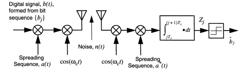
To illustrate the operation of a DS spread spectrum system, consider an information signal b(t). This signal may be a voice or data signal. We will assume that b(t) is a digital signal composed of a sequence of symbols, bj, each of duration Ts. The data signal is given by

where Ψ(t/T) is the unit pulse function:

This signal is multiplied by a spreading sequence a(t) which is composed of a sequence of chips:

where Tc is the chip period, and M is the number of PN symbols in the sequence before the sequence repeats. It should be noted that the chips serve to spread and identify the signal, whereas the data symbols convey information. In the IS-95 standard, spreading symbols are represented by quadrature chips having a carrier initial phase from the symbol set {ejπ/4, e−jπ/4, ej3π/4, e−j3π/4} [EIA93].
The multiplied signal, a(t)b(t), is upconverted to a carrier frequency fc by multiplying a(t)b(t) by the carrier,
Let us assume, for the moment, that the channel does not distort the signal in any way, so that the received signal, r(t), consists of a weighted version of the transmitted signal with added white Gaussian noise, n(t):
At the receiver, a local replica of the chip sequence, a(t − τ0), is generated, where τ0 is a random time offset between 0 and MTc. To despread the signal at the receiver, the local chip sequence must be “delay locked” with the received signal. This means that the timing offset, τ0, must be set to zero. One means of doing this is through the use of a Delay Locked Loop (DLL). Similarly, a Phase Locked Loop (PLL) may be used to create a replica of the carrier, cos(ωct). Using these two quantities, a decision statistic is formed by multiplying the received signal by the local PN sequence and the local oscillator and integrating the result over one data symbol:

Let us assume that a(t)a*(t) = 1, then

where η represents the influence of channel noise on the decision statistic. Assuming that the carrier frequency is large relative to the reciprocal of the bit period, then
Therefore, the decision statistic, Zj, is an estimate, ![]() , of the transmitted data symbol bj.
, of the transmitted data symbol bj.
If the channel noise is additive white Gaussian noise with two-sided power spectral density N0/2, then the variable η is a zero mean Gaussian random variable uη = 0 with variance

The energy per symbol of the signal component of the decision statistic, Zj, is
Let us assume that the symbols, bj, being transmitted are from a binary symbol set such that bj ∈ {−1, 1}. Then the energy per symbol, Es, in (1.11) is the same as the energy per bit, Eb. The bit error rate at the output of the matched filter receiver is given by

where Q(x) is the standard Q-function which is given in Appendix B. The Q-function is a monotonically decreasing function, so that a larger ratio of symbol energy to noise power produces a smaller bit error rate.
The bit error rate given by (1.12) is the same as if we had used no spreading sequence. However, there are several differences between this case and the case where no spreading sequence is used. First of all, since the signal is spread over a large bandwidth with the same total power, the spectral density of the signal can be very small. This makes it difficult for a potential eavesdropper to detect the presence of the signal. This property is known as Low Probability of Detection (LPD). Additionally, if the eavesdropper does not know the PN-sequence used, then it will be very difficult to extract the information signal portion of r(t). This property is called Low Probability of Interception (LPI) [Proa89].
In mobile and portable radio channels, the fact that the DS signal is spread over a large bandwidth can significantly mitigate the effects of fading which can degrade the performance of narrowband systems. The coherence bandwidth of the channel quantifies the region of spectrum over which the amplitudes of all signal components at the receiver undergo approximately the same fading level. Typical values for coherence bandwidth are 3 MHz in indoor channels and 0.1 MHz for outdoor channels [Rap96a]. If the signal bandwidth is smaller than the coherence bandwidth of the channel and one part of the spectrum of the signal experiences a fade, then, in all likelihood, the entire signal spectrum experiences a fade and it is not possible to recover the lost data symbols except through error control coding. Using DS techniques, the signal can be made to cover a large enough bandwidth so that if one part of the signal spectrum is in a fade, other parts of the signal spectrum are not faded. One result of this is that the short-time variation of the total received power for a wide band DS signal is much less than that of the narrowband signal [Ste92]. Various techniques can be used to recover the signal as long as some portion of the received signal is not in a fade.
Finally, one property of the DS signal alluded to earlier is that many DS signals can be overlaid on top of each other in the same frequency band. Let us assume that there are two users in the system using the same frequency band at the same time. We assume that the PN sequence from user 0 is a0(t) and the PN sequence from user 1 is a1(t) where

The signals are said to be orthogonal over a symbol period if

Let us assume for the moment that the repetition rate of the PN-sequence is the same as the symbol period such that MTc = Ts. When the length of the PN sequence, MTc, is equal to the message symbol period, Ts, the system is called a code-on-pulse system. If the sequences are chip aligned, and bit aligned, then the orthogonality over a symbol period may be expressed as

If each user has a different orthogonal underlying code sequence, then many users can share the same medium without interfering with each other. This property may be used as a multiple access technique, namely Code Division Multiple Access. The case in which the user’s sequences are chip and bit aligned is called synchronous CDMA.
The received signal at user 0’s receiver consists of the desired signal, multiple access interference from user 1, and noise
where

The decision statistic for user 0 is obtained using Equation (1.7). The component of the decision statistic due to the desired signal is A0Tsb0,j/2, just as before. The component of the decision statistic due to the noise component is again a zero mean Gaussian random variable with variance N0Ts/4. In synchronous CDMA, the component due to the interference is

Thus if the spreading sequences of user 0 and user 1 are orthogonal, so that they satisfy (1.15)ch01equ1,5 then the component of the decision statistic due to interference will be zero. In this case, the addition of the users in the same time and frequency slots will not affect the performance of other users. In most cases, it is possible to operate only in a synchronous CDMA mode on the forward link since the base station can simultaneously modulate and spread the signals for all users. On the reverse link, since it is difficult to synchronize spatially separated mobile users on the bit and chip level, and since the signals travel different path lengths from the transmitter to the base station, it is not feasible to operate in a synchronous mode.
In the asynchronous case, where usually the sequence for user 1 is delayed by τ1 seconds relative to the chip sequence for user 0, the expression describing the interaction between the signals from two users at the receiver for user 0 becomes considerably more complicated. We may express the delay as an integer number of chip periods γ1 such that τ1 = γ1Tc + Δ1 where 0 ≤ Δ1 < Tc. We will further assume that for values of i ≥ M and i < 0 that a1, i = a1, i−mM, so that 0 ≤ i − mM < M − 1. Then the signals from user 0 and 1 will not interfere with each other if

It is not possible to select useful spreading codes which satisfy (1.19) over all possible values of b1, j, Δ1 and γ1. Thus, in an asynchronous CDMA system, the signals from different users interfere with each other, resulting in higher bit error rates as compared with orthogonal CDMA. Therefore, in asynchronous CDMA systems, every user contributes interference, called Multiple Access Interference (MAI), to the decision statistic for other users.
Consider a CDMA system in which K users occupy the same frequency band at the same time. These users may share the same cell, or some of the K users may communicate with other base stations.
The signal received at the base station from user k is given by [Pur77]
where bk(t) is the data sequence for user k, ak(t) is the spreading (or chip) sequence for user k, τk is the delay of user k relative to a reference user 0, Pk is the received power of user k, and φk is the phase offset of user k relative to a reference user 0. Since τk and φk are relative terms, we can define τ0 = 0 and φ0 = 0.
Let us assume that both ak(t) and bk(t) are binary sequences having values of −1 or +1. As noted earlier, the IS-95 CDMA system, which we will discuss in the next section, uses a somewhat different waveform, with quadrature spreading. The binary values used here, however, are useful for demonstrating some fundamental concepts in DS-CDMA.
The chip sequence ak(t) is of the form,

where M is the number of chips sent in a PN sequence period and Tc is the chip period. MTc is the repetition period of the PN sequence.
For the data sequence, bk(t), Tb is the bit period. As noted in the introduction to this chapter, it is assumed that the bit period is an integer multiple of the chip period such that Tb = NTc. Note that M and N do not need to be the same. The binary data sequence bk(t) is given by

At the receiver, illustrated in Figure 1-12, the signal available at the input to the correlator is given by

![Model for CDMA multiple access interference [Pur77]](http://imgdetail.ebookreading.net/system_admin/3/0137192878/0137192878__smart-antennas-for__0137192878__graphics__01fig12.jpg)
where n(t) is additive Gaussian noise with two-sided power spectral density N0/2. It is assumed in (1.23) that there is no multipath in the channel with the possible exception of multipath that leads to flat fading such that the coherence time of the channel is considerably larger than a symbol period.
At the receiver, the received signal is mixed down to baseband, multiplied by the PN sequence of the desired user (user 0 for example) and integrated over one bit period. Thus, assuming that the receiver is delay and phase synchronized with user 0, the decision statistic for user 0 is given by

For convenience and simplicity of notation, the remainder of the analysis will be presented for the case of bit 0 (j = 0 in (1.24)). Substituting (1.20) and (1.23) into (1.24),

which may be expressed as
where I0 is the contribution to the decision statistic from the desired user (k = 0), ζ is the multiple access interference, and η is the noise contribution. The contribution from the desired user is given by

As shown in Appendix A, the noise term, η is given by

where it is assumed that n(t) is white Gaussian noise with two-sided power spectral density, N0/2. The mean of η is

From (1.10), the variance of η is
The third component in (1.26), ζ, represents the contribution of multiple access interference to the decision statistic. ζ is the summation of K − 1 terms, Ik,


If the spreading sequences are not orthogonal, then the cross correlation properties of the sequences determine the degree to which one DS signal interferes with another DS signal. For a given length of PN-sequence, there is generally a much larger number of different sequences with low cross-correlation properties than mutually orthogonal sequences. From (A.49), it follows that

where N is the spreading factor,
where Rc is the chip rate of the PN sequence and Rb is the message bit rate.
In Appendix A it is shown that, using the Gaussian Approximation, the Multiple Access Interference can be approximated as a Gaussian random variable. Then we approximate the Bit Error Rate using (A.51) as

in the interference limited case, where ![]() , this becomes
, this becomes

Consider the CDMA uplink where multiple subscribers are transmitting signals that are received at a single base station receiver. Generalizing (1.36), the bit error rate for user p can be expressed as
where N is the spreading factor and γp represents the Carrier-to-Interference-Ratio (CIR) for subscriber p. Letting Pp represent the received power from user p, γp is

As the CIR increases, the bit error rate for a subscriber decreases.
Recall that Pk represents the power received at the base station from a particular subscriber. If every user transmits at the same power level, then the received power from users closer to the base station will tend to be higher than the received power from subscribers that are farther away from the base station. This leads to a different performance for subscriber links, depending on where the subscribers are located in the cell. More importantly, a few subscribers closest to the base station may contribute so much Multiple Access Interference that they prevent other uplink signals from being successfully received at the base station. This is the near-far effect [Rap96a].
To solve this problem, power control is used in CDMA systems. Power control forces all users to transmit the minimum amount of power needed to achieve acceptable signal quality at the base station. Power control typically reduces the power transmitted by subscribers closest to the base station, while increasing the power of subscribers farthest away from the base station. Compared with the case where all users transmit at the same power level, power control reduces the denominator of (1.38), increasing the CIR, and lowering the error rate for all subscribers.
If all subscribers in a system have the same bandwidth, data rate, and other signal characteristics, then one reasonable approach to power control is to set all of the received power levels, Pk, to a constant value, Pc. Then (1.38) can be rewritten as
This is called perfect power control. In practice, this sort of perfect power control is not achievable and under many circumstances, despite its name, may not even be desirable.
Perfect power control requires exact knowledge of the loss in the radio propagation channel between the subscriber transmitter and the base station receiver, commonly referred to as path loss. As shown later in this chapter, there are a number of factors that impact the path loss between the transmitter and receiver, causing signal levels to fluctuate with time. In practical systems, the path loss between the uplink path is estimated through a combination of techniques. These include Open Loop Power Control, where the path loss on the downlink is measured, and it is assumed that the path loss is approximately the same on the uplink, so the subscriber unit adjusts its power accordingly. To account for the time varying nature of the channel, and the fact that path loss in the forward and reverse directions may not be the same, practical systems also use Closed Loop Power Control, where the base station instructs the subscriber unit to raise or lower its transmit power to meet some targeted received power level. This allows the mobile to adjust its transmit power to track the time varying nature of the channel.
Rather than adjust the subscriber transmitter power to meet a desired received power level at the base station, practical CDMA systems use other criteria for adjusting power levels. These include adjusting the power level to meet specific error rate or Carrier-to-Interference-and-Noise-Ratio (CINR) requirements. Chapter 2 illustrates that the IS-95 CDMA standard uses a complex power control mechanism that adjusts the subscriber transmitter power 800 times per second.
Assuming perfect power control, (1.36) can be used to illustrate how the addition of subscribers to a CDMA system increases the bit error rate seen by the receiver for any particular subscriber.
In the non-interference limited case, for perfect power control where Pk = P0 for all k = 0...K − 1, we have

In the interference limited case with perfect power control, equation (1.40) may be approximated by

Equation (1.41) is plotted in Figure 1-13. As the number of users increases, the raw bit error rate seen by the uplink receiver for any particular receiver increases. CDMA systems use error control coding so they are tolerant of bit errors introduced by Multiple Access Interference. Note that the agreement is excellent for average bit error rates larger than 10-3, where most voice systems operate. However, due to the tail of the Gaussian distribution, the approximation slightly over estimates capacity for bit error rates less than 10-3.
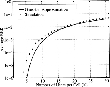
Figure 1-13. The bit error rate for an asynchronous reverse link obtained through computer simulation and through application of the Gaussian Approximation given in (1.41). The spreading factor is N = 31 and perfect power control is applied such that all users have the same power level. Omni-directional antennas are used at the base station.
An alternative to Direct Sequence (DS) is Frequency Hop Spread Spectrum (FH-SS). In many ways, these systems are similar to an FDMA system, in which the bandwidth available for multiple users is divided into N channels. At any point in time, a frequency hopping signal for a particular user occupies only a single frequency channel. The difference between this system and a traditional FDMA system is that the frequency hopping signal changes frequency carriers, or hops, at rapid periodic intervals. If the signal hops at, or close to, the symbol rate, the system is termed a fast frequency hopping system. If hopping occurs at a lower rate, it is called slow frequency hopping. The sequence of frequency slots occupied by the FH signal is a pseudo random sequence.
The pseudo random sequence is recreated at the receiver which retunes to the proper channel to match the transmitted signal. It is assumed that not all of the channels are continuously occupied. If two multiple access users are using the same channel set, each using a different pseudo random channel sequence, the signals will occasionally be transmitted in the same frequency slot. A bit error may occur in this case, but the effects of this can be minimized through the use of error control coding [Lin83][Rap96a].
A frequency hopping system provides a level of security, especially when a large number of channels are used, since an unintended receiver that does not know the pseudo random sequence of frequency slots must constantly retune to search for the signal that it is attempting to intercept. FH systems also have the effect of randomizing interference which can be beneficial [Par89]. In today’s emerging wireless CDMA technology, DS spread spectrum has been widely accepted, and the remainder of this text focuses on Direct Sequence rather than Frequency Hop Spread Spectrum.
In any wireless system, antennas are used at each end of the link. The antenna is a means of coupling radio frequency power from a transmission line into free space, allowing a transmitter to radiate, and a receiver to capture incident electromagnetic power. Antennas can be as simple as a piece of wire, or they can be complex systems with active electronics. Despite the range of technologies comprising antenna systems, there are a number of concepts which are common to all antenna systems.
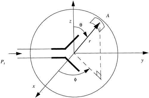
An antenna is illustrated in Figure 1-13. Here, a signal with time-average power of Pt is fed into the antenna. The antenna radiates this power in all directions. We define a direction using polar coordinates, θ and φ. If the vector r points in a particular direction, then φ is the angle between the x-axis and the projection of r into the x-y plane and θ is the angle between the z-axis and r.
The power density, having units of W/(rad)2, for a particular direction (θ, φ), is given by U(θ, φ). If the antenna is lossless, and perfectly matched, then all of the power, Pt, flowing into the antenna will be radiated. In this case, the total power transmitted in all directions is

The average power density, Uave, is

If the antenna transmits power equally in all directions, then U(θ, φ) will be equal to Uave, and the antenna is said to be isotropic. Isotropic antennas are useful for analytical purposes; however, most real antennas exhibit directionality, meaning that they transmit more power in one direction than in other directions. The maximum power density for the antenna is
We define the gain of an antenna, with respect to isotropic, as
where η is the efficiency of the antenna, which accounts for losses. G(θ,φ) is also called the antenna power pattern. The peak gain of the antenna is

When a single value is given for the gain of an antenna, it refers to the peak gain. The Effective Isotropic Radiated Power (EIRP) is defined as
The EIRP is the amount of power that would be required, using an isotropic antenna, to produce the same power density that is achieved in the boresight direction of the directional antenna. At a distance r from the antenna, in a direction (θ, φ), the total power available in an area, A is
In the direction of peak gain, total power available in an area A at a distance of r from the antenna is
Another important result is that the maximum gain of an antenna can be expressed in terms of its size or maximum aperture, Am,
where λ = c/f is the wavelength, with c, the speed of light, equal to 3 × 10⁸ m/s, and f is the carrier frequency in Hz. This expression states that for an antenna of size, or maximum aperture, Am, its gain will increase by the square of the frequency. Equivalently, the effective aperture, Ae = ηAm, is often used, where
Consider the wireless link illustrated in Figure 1-14. Here, a transmitter produces an RF signal with time-average power Pt, using an antenna with gain Gt. At the receiver, which is a distance d from the transmitter, an antenna with gain Gr is used.
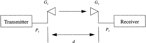
Let us assume that the transmitter and receiver antennas are pointing toward each other so that their boresights are aligned. Then using (1.48), the power available at the receiving antenna is

where Ae is the effective aperture of the receiving antenna. Using (1.51), the received power can be expressed as

This expression is Friis’ Free Space Link Equation. The transmit power is measured in watts, the wavelength and distance are measured in meters, and the received power is given in watts. It is usually much more convenient to work in decibel units where
where log(x) is the base 10 logarithm of x.
Here, Pr and Pt are measured in dBm, Gt and Gr are in dBi, d is measured in meters, f is the carrier frequency in Hz, and c is the speed of light, 3×10⁸ m/s. The received power in dBm is related to the received power in watts, Pw, by
The term dBi refers to the gain of an antenna, in dB, relative to an isotropic antenna. From (1.46), since Um = Uave for an isotropic antenna, if the antenna is lossless, then the gain of an isotropic antenna, Giso = 1. Therefore, the gain of an antenna relative to an isotropic antenna is
Throughout the remainder of this text, we will typically use the terms Pr, Pt, Gt, and Gr to refer to either power levels in dBm and gain in dBi or, alternatively, power levels in watts and gain as a unitless quantity.
Equation (1.54) has several important implications for wireless communication systems. For adequate performance of a radio link, there is a minimum received power level, Pr, that must be available at the receiver. Given a particular T-R separation, d, and a frequency of operation, f, there are three ways that we can increase Pr. One way is to increase the transmitter power Pt. If the transmitter is a portable unit, however, increased transmitter power can reduce battery life, and high-power transmitters can be expensive and bulky. Alternatively, we can increase the gain of the transmitting or receiving antennas.
At the subscriber end of a mobile link, antenna gain is limited by several factors. Usually, tiny portable subscriber antennas must be able to provide uniform performance, regardless of the orientation of the antenna or the subscriber. Therefore, relatively non-directional antennas with low gain are often used. Another important factor is shown by (1.51). Here we see that the gain of an antenna is limited by its size. In order to achieve substantial gain at the portable unit, at frequencies used for cellular and PCS systems, the small size of portable transceivers severely limits the maximum gain obtainable.
As an example, suppose that a gain of 6 dBi is required from an antenna operating at 1900 MHz. Using (1.51), we find that an aperture of at least 80 cm2 (8 cm × 10 cm) is required. This is much more than the area of a typical modern subscriber transceiver. Note, however, that wireless systems using antennas on cars, or Wireless Local Loop systems, which use antennas mounted on a residence, are important exceptions where larger antennas are possible.
For base stations, using conventional antennas with fixed antenna patterns, gain is usually limited to approximately 16-20 dBi. This is because base stations using conventional antennas must be able to supply adequate power throughout a coverage area. Smart antenna systems can offer improvements by offering dynamic antenna patterns.
We should note some key limitations and assumptions of Friis’ Free Space Link Equation. First of all, as the name implies, the expression applies only in free space. Equation (1.54) does not account for multipath, or obstructions between the transmitter and receiver. We can generalize Friis’ link equation by writing (1.54) as
where Lp represents the path loss between the transmitter and receiver.
The mechanisms behind electromagnetic wave propagation are diverse, but they can generally be attributed to reflection, diffraction, and scattering. Most cellular radio systems operate in urban areas where there is often no direct line-of-sight path between the transmitter and the receiver, and where the presence of high-rise buildings causes severe diffraction loss. Due to multiple reflections from various objects, the electromagnetic waves travel along different paths of varying lengths. The interaction among these waves causes multipath fading, and the strengths of the waves decrease as the distance between the transmitter and receiver increases.
Propagation models have traditionally focused on predicting the average received signal strength at a given distance from the transmitter, as well as the variability of the signal strength in close spatial proximity to a particular location. Propagation models that predict the mean signal strength for an arbitrary transmitter-receiver (T-R) separation distance are useful in estimating the radio coverage area of a transmitter and are called large-scale propagation models, since they characterize gross path loss characteristics that apply over scales that are large compared to a wavelength. On the other hand, propagation models that characterize the rapid fluctuations of the received signal strength over very short travel distances (a few wavelengths) or short time durations (on the order of seconds) are called small-scale or fading models.
As a mobile moves over very small distances, the instantaneous received signal strength may fluctuate rapidly, giving rise to small-scale fading. The reason is that the received signal is a sum of many contributions coming from different directions. Since the phases are random, the sum of the contributions varies widely; for example, a CW or narrowband signal obeys a Rayleigh fading distribution. In small-scale fading, the received power of a narrowband signal may vary by as much as three or four orders of magnitude (30 or 40 dB) when the receiver is moved by only a fraction of a wavelength. However, the local average signal power will be constant over a distance of several meters. As the mobile moves away from the transmitter over much larger distances, the local average received signal power will gradually decrease; it is this local average signal level that is predicted by large-scale propagation models. Typically, the local average received power is computed by averaging signal measurements over a measurement track of 5λ to 40λ in a local area. For cellular and PCS frequencies in the 1 GHz to 2 GHz band, this corresponds to measuring the local average received power over movements of 1 m to 10 m.
In wideband CDMA systems where the RF bandwidth exceeds the coherence bandwidth of the channel (or alternatively, when the chip duration is smaller than the multipath channel delay spread), the received signal power fades much less than a narrowband signal, as shown in Figure 1-16.
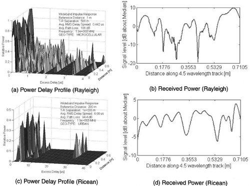
Figure 1-16. Plots showing the power delay profile and received power as a receiver moves over a 0.6 meter track. In the Rayleigh fading environment, shown in (a) and (b), many multipath components can combine destructively, resulting in deep fades in the total received power. In (c), the fact that very few later arriving components are weaker than earlier components leads to less deep fades, as illustrated in (d). These channels were simulated using SMRCIM 3.0.
Most large scale radio propagation models are derived using a combination of analytical and empirical methods. The empirical approach is based on fitting curves or analytical expressions that recreate a set of measured data in the environment of interest. This approach has the advantage of implicitly taking into account all propagation factors, both known and unknown, through actual field measurements. However, the validity of an empirical model at transmission frequencies or environments other than those used to derive the model can be established only by additional measured data in the new environment at the required transmission frequency. Over time, some classical propagation models have emerged which are now used to predict large-scale coverage for wireless communication systems design. By using path loss models to estimate the received signal level as a function of distance, it becomes possible to predict the Carrier-to-Noise-Ratio for a mobile communication system.
Both theoretical and measurement-based propagation models indicate that average received signal power decreases by the logarithm of the distance between the transmitter and the receiver, whether in outdoor or indoor radio channels. Such models have been used extensively in the literature. The average large-scale path loss for an arbitrary T-R separation is expressed as a function of distance by using a path loss exponent, n.
or
where n is the path loss exponent which indicates the rate at which the path loss increases with distance, d0 is the close-in reference distance which is determined from measurements close to the transmitter, and d is the T-R separation distance. The bars in equations (1.58) and (1.59) denote the ensemble average of all possible path loss values for a given value of d. When plotted on a log-log scale, the modeled path loss is a straight line with a slope equal to 10n dB per decade. The value of n depends on the specific propagation environment. For example, in free space, n is equal to 2, and when obstructions are present, n will have a larger value.
It is important to select a free space reference distance that is appropriate for the propagation environment. In large coverage cellular systems, 1 km reference distances are commonly used [Lee89], whereas in microcellular systems, much smaller distances (such as 100 m or 1 m) are used. The reference path loss is calculated by using the free space path loss formula given by equation (1.54) or through field measurements at distance d0. Table 1-5 lists typical path loss exponents and log normal shadowing standard deviations obtained in various mobile radio environments.
Table 1-5. Path Loss Exponents and Log-normal Shadowing Standard Deviation for Different Environments [Rap96a]
The model in equation (1.59) does not consider the fact that the surrounding environmental clutter may be very different at two different locations having the same T-R separation. This leads to measured signals which are much different than the average value predicted by equation (1.59). Measurements have shown that at any value of d, the path loss PL(d) at a particular location is random and distributed log-normally (normal in dB) about the mean distance-dependent value [Cox84], [Ber87]. We can therefore express the path loss as
and
where Xσ is a zero-mean Gaussian distributed random variable (in dB) with standard deviation σ (also in dB).
The log-normal distribution describes the random shadowing effects which occur over a large number of measurement locations which have the same T-R separation, but have different levels of clutter on the propagation path. This phenomenon is termed log-normal shadowing. Simply put, log-normal shadowing implies that measured signal levels at a specific T-R separation have a Gaussian (normal) distribution about the distance-dependent mean of (1.59), where the measured signal levels have values in dB units. The standard deviation of the Gaussian distribution that describes the shadowing also has units in dB. Thus, the random effects of shadowing are accounted for, using the Gaussian distribution which lends itself readily to evaluation.
The close-in reference distance d0, the path loss exponent n, and the standard deviation σ, statistically describe the path loss model for an arbitrary location having a specific T-R separation; this model may be used in computer simulation to provide received power levels for random locations in communication system design and analysis. An example of an IS-95 link design using (1.60) is provided in Chapter 2.
In practice, the values of n and σ are computed from measured data, using linear regression where the difference between the measured and estimated path losses is minimized in a mean square error sense over a wide range of measurement locations and T-R separations. The value of ![]() in (1.60) is based on either close-in measurements or on a free space assumption from the transmitter to d0. An example of how the path loss exponent is determined from measured data follows. Figure 1-17 illustrates actual measured data in several cellular radio systems and demonstrates the random variations about the mean path loss (in dB) due to shadowing at specific T-R separations.
in (1.60) is based on either close-in measurements or on a free space assumption from the transmitter to d0. An example of how the path loss exponent is determined from measured data follows. Figure 1-17 illustrates actual measured data in several cellular radio systems and demonstrates the random variations about the mean path loss (in dB) due to shadowing at specific T-R separations.
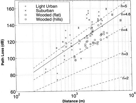
Figure 1-17. Plot of Path Loss vs. Distance at 1900 MHz for measurements performed with a receiver at microcell antenna heights (13 meters), and a mobile transmitter with an antenna height of 1.5 meters, in several different cluttered environments. The MMSE estimated path loss exponent for the collection of measurements is n = 4.6 with σ = 12.5 dB.
Since PL(d) is a random variable with a normal distribution in dB about the distance-dependent mean, so is Pr(d), and the Q-function or error function (erf) may be used to determine the probability that the received signal level will exceed (or fall below) a particular level. The Q-function is defined as

where
The probability that the received signal level will exceed a certain value γ can be calculated from the cumulative density function as
Similarly, the probability that the received signal level will be below γ is given by
Usually, shadowing is taken into account by determining a link margin that is required to achieve a certain coverage probability. For example, to achieve a 95% coverage probability at the cell edge with a shadowing standard deviation of σ = 10 dB, we find that we need ![]() or 16.5 dB. In other words, there is only a 5% probability that Pr(d) will be less than γ, as long as the mean received power,
or 16.5 dB. In other words, there is only a 5% probability that Pr(d) will be less than γ, as long as the mean received power, ![]() , is 16.5 dB above γ. We call this 16.5 dB value the shadowing margin. The link budget example in Chapter 2 uses shadowing margins to account for coverage probability due to shadowing.
, is 16.5 dB above γ. We call this 16.5 dB value the shadowing margin. The link budget example in Chapter 2 uses shadowing margins to account for coverage probability due to shadowing.
In this chapter, we presented an overview of several state-of-art technologies in wireless technology, including several important emerging systems such as Wireless Local Loop, LMDS, and Third Generation Wireless Systems. We also developed a foundation in CDMA technology, and provided concepts in antennas and propagation. These tools will allow the reader to delve into the details of smart antennas for CDMA in Chapters 3 and 4. First, however, we take a detailed look at the most widely deployed CDMA technology, IS-95, in Chapter 2.