
In this chapter, analytical tools are developed to study the performance of CDMA cellular radio systems which use spatial filtering, as well as to determine practical limits on the number of simultaneous active users that can be supported in these systems. In later chapters, we discuss spatial signal processing techniques used to implement CDMA spatial filtering. However, before delving into details on how to implement smart antennas for CDMA, it is useful to examine the potential performance improvements expected. Because this is vital for determining system benefits and cost justification for smart antennas, we take several approaches to analyze these systems. First, we examine a single cell to develop simple rules and general design guidelines for uplink capacity improvement using CDMA technology. Next, we consider the impact of out-of-cell interference on CDMA performance and discuss the impact of spatial filtering on these systems. We then look at fixed wireless systems to discuss the potential for smart antennas at the subscriber end of the link. We conclude by formulating an alternative approach to CDMA capacity improvement calculations.
In this chapter, we present computer simulations and analytical results which demonstrate that spatial filtering at the base station significantly improves the reverse channel performance of multi-cell mobile radio systems, and we derive analytical techniques for characterizing mobile radio systems which employ frequency reuse. Finally, we also discuss the effects of using spatial filtering at the portable unit.
An important benefit of smart antennas is range extension. Range extension allows the mobile to operate farther from the base station without increasing the uplink power transmitted by the mobile unit or the downlink power required from the base station transmitter.
First, consider the reverse link case of a single plane wave from a subscriber transmitter incident on the array. As described in Section 3.3, the data vector is equal to
The vector n(t) contains the noise contributed at each antenna element. Each element of n(t) is a complex Gaussian random variable with variance ![]() .
.
We can use (3.32) to find an optimal solution for the weight vector to extract s(t).
With some rearranging, we have
so w ∝ a(θ, φ), where the proportionality constant is unimportant. For simplicity, we set
Then the output of the antenna combiner, illustrated in Figure 3-3, is

The power of the desired signal component of z(t) is
The power of the noise component of z(t) is

Therefore, the signal to noise ratio of z(t) is
If, instead of using the array of M elements, only the signal at a single array element, uo(t), is used, then
The signal-to-noise ratio of uo(t) is
Comparing (5.8) and (5.10), we see that an M-element array can achieve an SNR improvement of
in Additive White Gaussian Noise (AWGN) with no interference or multipath. This is the signal-to-noise ratio improvement provided by the array relative to the signal-to-noise ratio at a single element.
Next, consider the CDMA reverse link budget in Table 5-1, which shows both the smart antenna uplink and the uplink using a conventional base station antenna. For this example, we assume that the standard deviation, σ, of the shadowing component, χσ, in (1.58) is 8dB. Using (1.63), with a single base station receiver, a shadowing margin of 1.28σ, or 10.2 dB, is received to achieve a 10% probability of outage due to shadowing. As shown in Section 2.2.1, using two-way soft handoff, the required link margin is reduced to 0.77σ, or 6.2 dB, while maintaining the same outage probability.
Table 5-1. Example of the uplink range extension achieved in a CDMA system using an 8 element array.
Conventional Sectoring | Smart Antenna System | |
|---|---|---|
Portable Tx Power (Class II):........................................(a). | 23.0 dBm | 23.0 dBm |
Portable Tx Antenna Gain:............................................(b). | 0.0 dBi | 0.0 dBi |
EIRP:...................................................................(c=a+b) | 23.0 dBm | 23.0 dBm |
BS. Antenna Element Gain (120° sector):......................(d) | 18.0 dBi | 18.0 dBi |
Ideal Spatial Processing Gain for M=8:..........................(e) | 9.0 dB | |
Total Receiver Antenna Gain:................................(f=d+e) | 18.0 dBi | 27.0 dBi |
Required CINR at correlator input:...............................(g) | -12.3 dB | -12.3 dB |
Receiver noise floor at NF=5 dB:.................................(h) | -108.1 dBm | -108.1 dBm |
Total noise and interference at χ = 0.9 ..........................(i) | -98.1 dBm | -98.1 dBm |
Shadowing margin (10% outage probability, for two-way | ||
Soft Handoff, σ=8 dB)...........................................(j) | 6.2 dB | 6.2 dB |
Req’d Median Received Power:........................(k=g+i+j) | -104.2 dBm | -104.2 dBm |
Tolerable Median Path Loss:..............................(l=c+f-k) | 145.2 dB | 154.2 dB |
Range, using a dn model with n=2 up to 0.5 km, n=4.5 for greater distances, with fc=1920 MHz:............................... | 7.7 km | 12.2 km |
We use a loading factor χ to account for multiple access interference from both in-cell and out-of-cell users [Vit95]. This will be discussed at greater length in Section 5.5. As shown in Table 5-1, the array is able to provide a 60% range improvement with no increase in transmitter power, or per-channel noise performance at the receiver, because M = 8 elements provide 9 dB more link margin, compared with conventional sectoring.
As a general rule-of-thumb, for a constant path loss exponent of n ≥ 2, the range of a cell using smart antennas, Rs, is greater than the range using conventional antennas, Rc, by
and the ratio of the area of a cell covered with smart antennas, As, to the area of a cell covered using conventional antennas, Ac, is
Therefore, if Nc conventional base stations are required to provide coverage to an area, then the same area can be served using Ns = Nc M(−2/n) base stations. For a path loss exponent of n = 4.5, using eight-element arrays, this means that the area can be covered using 60% fewer base stations than would be required using conventional antenna systems. This is a powerful economic argument for service providers to consider smart antennas.
Table 5-1 may be overly optimistic because the gain of each individual array element will most likely be less than the 18 dBi afforded by a large (1.5 m) sector antenna. It is often not feasible to mount eight large sector panel antennas on a cell face. If the gain of each array element is reduced to 15 dBi, then the range of the smart antenna system in Table 5-1 is reduced to 10.3 km. Despite this decreased range, 44% fewer base stations are required relative to conventional sectored antenna systems.
This example does not take into account the fact that the tele-density, or erlangs of traffic supported per square kilometer, will be lower using a sparse smart antenna-based layout compared with a dense deployment using conventional base stations. However, in early deployments, or in rural areas, tele-density may not be a concern. In the next several sections, we show how smart antennas can also be used to increase the number of simultaneous subscribers that can be supported in each cell. Combining these capacity improvement techniques with the range extension discussed in this section, and given the high cost of base station towers, and difficulty in accessing tower sites, fewer base stations with more channels per base station could provide comparable tele-density to conventional deployments. However, one should be careful not to overestimate the ability of adaptive arrays to fulfill simultaneous range extension and capacity improvement goals. The practical limitations of the adaptive antennas technology along with the air interface standard must be taken into account. As we will see in the next several sections, smart antennas can also significantly improve system capacity in dense deployments where high tele-density is required.
Consider a single cell CDMA system in which K mobile units simultaneously transmit to a single base station. This is a fundamental step toward developing concepts that will allow the multi-cell analysis required to predict CDMA capacity. As shown in Section 1.3.1, for interference limited, asynchronous, BPSK-CDMA over an Additive White Gaussian Noise (AWGN) channel, operating with perfect power control and with omni-directional antennas used at the base station, the bit error rate (BER), Pb, on the reverse link is approximated by [Pur77]
where K is the number of users in a cell and N is the spreading factor given in (1.35). Equation (5.14) assumes that the signature sequences are random and that K is sufficiently large to allow the Gaussian Approximation (GA) described in [Pur77] to be applied. Appendix A provides a thorough treatment of the Gaussian Approximation, as well as extensions that support analysis when users are not power-controlled.
In IS-95-based CDMA systems, (5.14) is not directly applicable because the uplink bit error rate is a complex function of different error control coding methods, orthogonal 64-ary modulation, multiple spreading codes, power control, and other factors. In IS-95, as described in Chapter 2, signals use modified M-sequences for short code and long code spreading. Offset-QPSK is used for spreading with BPSK data, and Data Burst Randomization helps to further randomize interference.
In IS-95 based systems, a critical parameter to measure link performance is the Carrier-to-Interference-and-Noise-Ratio (CINR) available for each subscriber. The CINR for each subscriber is measured after despreading. On the reverse channel, the CINR for a particular subscriber is measured at the input to the Walsh Chip Matched Filter, at the base station, as shown in Figure 4-3.
We define the CINR after despreading, as the ratio of the desired signal to the sum of interference and noise.

This is essentially the argument of the Q-function in (1.36).
In (5.15), P0 is the power of the desired signal at the input to the despreader at the base station, and Pk is the power from every other user for k = 1...K - 1. The spreading factor is given by N, which was defined in (1.35) as
Equation (5.15) reflects the fact that spreading reduces the impact of multiple access interference, Pk. The noise variance, ![]() , as in Section 1.3.1, represents the noise contribution to the decision variable after despreading.
, as in Section 1.3.1, represents the noise contribution to the decision variable after despreading.
Multiplying the numerator and denominator of (5.15) by the bit duration, Tb, we have

The term P0 T0 is the energy per bit for the desired subscriber signal. After despreading, the noise bandwidth is approximately 1/Tb. If the thermal noise has a power spectral density of Nn, then we can write the CINR as

The term Ni represents the power spectral density of the total multiple access interference after despreading.
Rather than using the spreading factor, as defined in (5.16), to compute the CINR in complex systems such as IS-95, it is more appropriate to compute the CINR using the processing gain. The processing gain for IS-95 systems results from a combination of PN-spreading and convolutional coding. This is because, as with PN-sequence spreading, convolutional coding increases the number of channel symbols compared with the number of information bits, and provides protection from the effects of MAI.
For the IS-95 uplink, the chip rate is 1.2288 Mcps. For both Rate Set 1 and Rate Set 2, the maximum symbol rate out of the convolutional encoder is 28.8 ksps. Therefore, the spreading factor is
or 16.3 dB. A common practice in IS-95 systems is to include also the impact of convolutional encoding in the processing gain. In Rate Set 1, which uses a 1/3 rate convolutional encoder on the reverse link, the processing gain is
or 21.1 dB. For Rate Set 2, using the 1/2 rate coder, the processing gain is 42.667 × 2 = 85.333 or 19.3 dB. These rates also correspond to the ratio between the chip rate and the basic information rates of 9600 bps and 14400 bps, respectively, for each Rate Set, as shown in Tables 2-9 and 2-10. Therefore, we will use the term, N, to refer to the processing gain in (5.18).
As discussed in Chapter 2, the power control scheme in IS-95 uses Outer Loop Power Control to adjust the Frame Error Rate (FER) to a target value, typically 1%. The CINR required to deliver this FER is a function of rate set, vehicle speed, multipath conditions, and soft/softer handoff state. As described in Chapter 2, when linking to a single base station, for mobile subscribers, an Eb/N0 of 7-9 dB is required. Using soft handoff, the value of Eb/N0 required at each receiving base station drops to 4-6 dB due to macro-diversity that reduces the impact of shadow fading [Ket96][Wal94].
It is also important to account for the fact that IS-95-based CDMA systems take advantage of voice inactivity as described in Section 2.3.1. Because the vocoder reduces its output rate when the speaker is silent, the subscriber unit does not transmit continuously, but is gated on and off with a duty cycle as low as 1/8 during silent periods. This is captured in the voice activity factor, ν. Typically, the voice activity factor reduces the average Multiple Access Interference level seen by the base station receiver by 50-60% (ν =0.4 to 0.5) relative to the case where all subscribers are transmitting continuously.
We can modify (5.18) to take into account the CINR improvement due to the voice activity factor:

To illustrate how directional base station antennas can improve the reverse link in a single cell CDMA system, consider the case in which each portable unit has an omni-directional antenna and the base station tracks each user in the cell, using a directive beam. It is assumed that a beam pattern, F(θ, φ), is formed at the base station so that the pattern has a steerable maximum in the direction of the desired user. For this analysis, we will assume that F(θ, φ) is a keyhole pattern, as shown in Figure 5-1. This pattern, which resembles a keyhole when its cross-section is viewed in the x-y-plane, is not physically realizable, but it is useful for analysis.
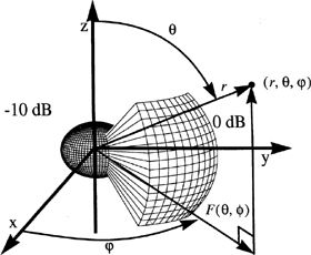
We will assume that the pattern is separable in the θ (elevation) and φ (azimuth) dimensions, so that we can express the pattern as
The elevation pattern, Fe(θ), is fixed with a maximum value on the horizon, at θ = π/2. For simplicity, we will assume that
The maximum gain of the overall pattern, given by (1.44), is

When considered by itself, the maximum gain of the elevation pattern portion of the separable antenna pattern, Fe(θ), is

The azimuth pattern, Fa(φ), can be steered through 360 degrees in the horizontal (φ) plane so that the desired user (user 0) is always in the main beam of the pattern. The maximum value of the horizontal antenna pattern occurs in the direction toward user 0.
The maximum gain of the horizontal portion of the pattern, Fa(φ), is

We assume that K users in the single cell CDMA system are uniformly distributed throughout a two-dimensional cell (in the horizontal plane, θ = π/2). On the reverse link, the received power from the desired mobile is Pr;0. The powers of the signals incident at the base station antenna from the K – 1 interfering users are given by Gm Fα(φi)Pr;i where φi is the direction of the ith user in the horizontal plane, measured from the x-axis. Then the average total interference power, Io, seen by the base station receiver for user 0, measured at the output of the receiving array, is given by

If perfect power control is applied so that the power incident at the base station antenna from each user is the same, then Pr;i = Pc for each of the K users, and the average interference power seen by user 0 is given by

Assuming that users are independently and identically distributed throughout a circular region with radius R, the average total interference power received at the central base station may be expressed as

where fr,φ(r,φ) is the probability density function describing the geographic distribution of users throughout the cell. Assume users are uniformly distributed in the cell, then we have
and

Substituting (5.26) into (5.31) we have
Assuming that the system is set to operate with ![]() , so that the system is not thermal noise-limited, then the mean CINR is found from (5.21)
, so that the system is not thermal noise-limited, then the mean CINR is found from (5.21)

In other words, the CINR is proportional to the gain associated with the horizontal portion of the antenna pattern, Fa(φ). Note that (5.33) holds for a single cell CDMA system, with perfect power control applied to all subscribers, when the base station antenna pattern may be steered toward the desired subscriber.
With the canonical single-cell CDMA system with perfect power control as a backdrop, we now explore capacity limitations of multi-cell CDMA systems. Section 5.3 describes analytical techniques used to determine bit error rates in multi-cell CDMA systems employing spatial filtering. These techniques are applied to compare the performance of omni, sectorized, and smart antenna systems at the base stations. In Section 5.4, the effects of spatial filtering at the subscriber unit are examined, using several different base station configurations.
In this section, we investigate how smart antennas are used on the reverse link to improve CDMA system capacity in multi-cell systems. Note that equation (5.33) is valid only when a single cell is considered. To study the effects of spatial filtering on the reverse link when CDMA users are simultaneously active in several adjacent cells, we must first define the geometry of the cell region. For simplicity, we consider the geometry proposed in [Rap92][Rap96a] with a single layer of surrounding cells, as illustrated in Figures 5-2 and 5-3.
![The wedge cell geometry proposed in [Rap92], showing a central cell surrounded by eight wedge-shaped cells that have the same area as the central cell.](http://imgdetail.ebookreading.net/system_admin/3/0137192878/0137192878__smart-antennas-for__0137192878__graphics__05fig02.jpg)
Figure 5-2. The wedge cell geometry proposed in [Rap92], showing a central cell surrounded by eight wedge-shaped cells that have the same area as the central cell.
To develop a framework for studying CDMA systems, first consider the simple case where omni-directional antennas are used at each base station. Each antenna pattern is assumed to be of a separable form, as shown in (5.22), so that it can be expressed as F(θ, φ) = Fa(φ)Fe(θ). For an omni-directional antenna, Fa(φ) = 1 for all φ. Using (5.26), the azimuthal gain is Ga = 1, so that the overall antenna gain is Gm = Ge.
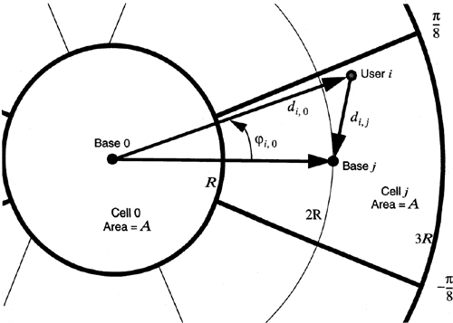
Let di, j represent the distance from the ith user to base j as illustrated in Figure 5-3. Let di, 0 represent the distance from the ith user to base station 0, the center base station. If Cell 0 contains the desired user, user 0, then the ith user shown in Figure 5-3 is an in-cell interferer if it is in Cell 0, and it is an out-of-cell interferer if it is outside of Cell 0. If user i is outside of Cell 0, then that user is power controlled to a base station in another cell j, and it represents a source of uplink interference that is not under control of the center cell.
Assume that the subscriber unit uses an isotropic antenna with a gain of Gsub = 1. The path loss between user i and base j is given by the log-distance path loss model described in Section 1.7.1, so that the power received at base station j, from the transmitter of user i, Pr, i, j, is given by

where n is the path loss exponent, and dref is a close-in reference distance [Rap92]. The term Li, j represents a log-normally distributed shadowing loss on the link between subscriber transmitter i and base station receiver j.
Assume that base station j applies perfect power control to all users in cell j, so that power Pc, j is received at base j, for each of the users in cell j, then the required power transmitted by user i, Pt;i, is

The power received at base station 0 from user i, Pr;i,0 is given by
Substituting (5.35) into (5.36), the reverse link power received at base 0 from user i, in adjacent cell j, is
To analyze (5.37), we consider the geometry shown in Figure 5-3. From the law of cosines,
Substituting (5.39) into (5.38), the power received at base 0 from user i is
To determine the average out-of-cell interference power incident on the central base station, we assume that users are uniformly distributed in a typical adjacent cell from r=R to r=3R and from φ = π/8 to π/8. Thus, we use a modified geometry from [Rap92] where 8 equal area cells surround the center cell. The probability density function (pdf) for the spatial distribution of users in a single adjacent cell is given by
Note that [Rap92] also considers the case in which users are not uniformly distributed throughout the cell. By allowing more users in an adjacent cell to concentrate closer to the central cell (in the smaller portion of the wedge), system performance is degraded [Rap92]. This is because out-of-cell users must transmit more power to reach their own base station, while generating more interference to the central base station due to their proximity. In this way, a worst-case analysis may be performed. For the present analysis, we consider only the case in which all users are uniformly distributed throughout the available coverage region.
Let ξ represent the expected value of the interference power from a single user in one of the adjacent cells when omni-directional base station antennas are used.

The terms Li, 0 and Li, j are independent and log-normally distributed, with E[Li, 0] = E[Li, j], so E[Li, 0/Li, j] = 1. If it is assumed that the center base station and all 8 surrounding base stations control power such that Pc;j = Pc, then, given a path loss exponent of n, we can express the expected value of central cell interference power from a single adjacent cell user as
where

Table 5-2 lists values of β for several values of n.
Table 5-2. Values of β as a function of the path loss exponent, n as determined by (5.43).
n | β |
|---|---|
2 | 0.1496 |
3 | 0.0824 |
4 | 0.0551 |
When omni-directional antennas are used at both the base station and the portable unit, β is related to the reuse factor, f, where f ≤ 1. The reuse factor is defined in [Rap92] as the ratio of received power from all in-cell interferers to the total interference from all users, with the assumption that users are in perfect power control to their closest base station.
As described in Chapter 8 of [Rap96a], this reuse factor is equivalent to the reciprocal of the frequency reuse ratio used in FDMA and TDMA systems.
For a single layer of adjacent cells, as shown in Figure 5-2,
The term N0 in (5.45) is the total Multiple Access Interference, seen at the central base station on the reverse link due only to subscribers in the central cell. Na 1 is the total interference affecting the desired central cell user from all users in a single adjacent cell. M1 is the number of cells which are adjacent to the central cell, which is always 8 for the geometry considered in this chapter.
When power control is performed by each base station on its own users, so that the power received from each mobile unit in the base station controlling that unit is Pc, then (5.45) may be expressed as
where we assume that there are K users in each of the nine cells. For n = 4, from Table 5-2, β = 0.055, and, from (5.46), f = 0.69, meaning that 31% of the interference power received at the central base station is due to users in adjacent cells. The reuse factor is summarized in Table 5-3 for different path loss exponents and different cell geometries. The table illustrates the impact of out-of-cell interference in CDMA systems.
Table 5-3. Reuse factor as a function of path loss exponent. The reuse factor is the fraction of Multiple Access Interference, seen at the base station, that is due to in-cell subscribers.
n | Reuse Factor, computed using concentric circle cell geometry with a single tier of adjacent cells. (5.46) | Reuse Factor, computed using concentric circle cell geometry with three tiers of adjacent cells [Rap92] | Reuse Factor, computed using 36 hexagonal cells [Lib96c] |
|---|---|---|---|
2 | 0.46 | 0.19 | 0.17 |
3 | 0.60 | 0.37 | 0.34 |
4 | 0.69 | 0.49 | 0.48 |
When omni-directional antennas are used at both the base station and the portable unit, the total interference seen on the reverse link by the central base station is the sum of the interference from users within the central cell, (K – 1)Pc, and from users in adjacent cells, 8KβPc.

Now consider what happens as directional antennas are added at each base station. A horizontal beam pattern, Fa; i, j(φ), is applied for each subscriber and steered so that the desired subscriber is centered in the main beam of the pattern. As in the previous section, we assume the keyhole pattern of Figure 5-1 with the same beamwidth for each subscriber, so that the overall base station antenna gain is equal to Gm = Ge Ga for all links. We assume that the same value of elevation gain Ge is used from the previous example.
Now assume that all adjacent cell subscribers are power controlled to the same level Pc, j at base station j; however, the output power for each subscriber may be lower than the case using omni-directional antennas, due to increased gain, Gm for each subscriber, relative to Ge.
Let us assume that for the ith user in the central cell, an antenna beam from the central base station with pattern Fi, 0(θ, φ) = Fe(θ)Fa; i; 0(φ) may be formed with maximum gain in the direction of user i. The pattern for the desired user (user 0) is F0, 0(θ, φ) = Fe(θ)Fa; 0; 0(φ). For simplicity, we write this pattern for user 0 as F(θ, φ) = Fe(θ)Fa(φ).
The average interference power contributed by a single user in the central cell is thus given by

The average interference power at the array output of the antenna array at the base station due to a single user in an adjacent cell is given by

If Fa(φ) is piece-wise constant over the region (2p − 1)(π/8)< φ < (2p + 1)(π/8) for p = 0...7, then the antenna pattern may be expressed as

where

Substituting (5.50) into (5.49), we obtain

The gain, Ga of Fa(φ), as described by (5.50) is

Therefore, (5.52) may be rewritten, using (5.53) and (5.43), as
It can be shown that (5.54) remains valid when the beam pattern, G(φ), is rotated in the φ plane. Therefore, (5.54) is appropriate when G(φ) is piece-wise constant over (2p − 1)(π/8) < φ − φd <(2p +1)(π/8) for any angle φd between − π/8 and π/8.
Using (5.54) with (5.48), the total interference power at the array output of the center base station receiver is
which is 1/Ga times the interference received at an omni-directional base station, which was given by (5.47).
We can substitute (5.55) into (5.18) to obtain
Equation (5.56) shows how the azimuthal antenna pattern and the reuse factor combine to determine the CINR for a desired subscriber. The reuse factor is determined through the value of β, given in Table 5-2. It is assumed that perfect power control is applied as described in Section 5.2, with all base stations controlling reverse link received power to the same level, Pc.
To explore how (5.56) can be used to determine the capacity of a CDMA system, consider the three hypothetical base station antenna patterns illustrated in Figure 5-4. Descriptions of these patterns are summarized in Table 5-4. These antenna patterns are assumed to be directed so that maximum gain is in the direction of the desired mobile users. The first base station antenna pattern is an omni-directional pattern which models antennas used in traditional cellular systems. This configuration, shown in Figure 5-4(a) is used as a model for standard omni-directional systems without spatial filtering. This is Case A in Table 5-4.
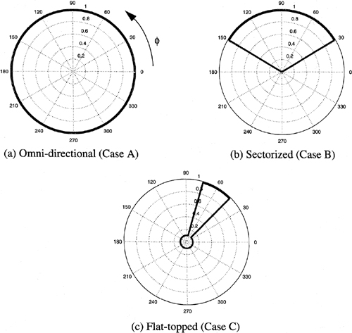
Table 5-4. Summary of the spatial filters used in this analysis.
Name | Ga | Description |
|---|---|---|
Case A: Omni-directional | 0 dB | Pattern is illustrated in Figure 5-4(a). |
Case B: Sectorized | 4.8 dB | Perfect 120° sectorization with zero sidelobes, shown in Figure 5-4(b). |
Case C: Flat-topped | 9.3 dB | Uniform gain across the 30° main beam and uniform sidelobes which are 10 dB below the main beam, as shown in Figure 5-4(c). |
The second configuration, given as Case B in Table 5-4 and illustrated in Figure 5-4(b), uses 120° sectorization at the base station. In this case, each base station uses three sectors, one covering the region from 30° to 150°, the second covering the region from 150° to 270°, and the third covering the region from −90° to 30°. The first sector is illustrated in Figure 5-4(b). This sector is active when the desired user is at an angle of 30° to 150°. The azimuth gain, Ga, of this antenna is 4.8 dB.
Table 5-5. Number of users supported in each cell, as limited by the reverse link for each spatial pattern. It is assumed that an Eb/N0 of 9 dB is required, and a voice activity factor of 0.6 is used.
Rate Set 1(N=19.3 dB) | Rate Set 1 (N=21.1 dB) | ||||||
|---|---|---|---|---|---|---|---|
Name | Ga | n=2 | n=3 | n=4 | n=2 | n=3 | n=4 |
Case A: Omni-directional | 0 dB | 12 | 16 | 18 | 8 | 10 | 12 |
Case B: Sectorized | 4.8 dB | 36 | 48 | 55 | 24 | 32 | 37 |
Case C: Flat-topped | 9.3 dB | 104 | 137 | 158 | 69 | 91 | 105 |
The third base station antenna pattern, shown in Figure 5-4(c), uses a flat-topped beam pattern similar to that shown in Figure 5-1. The main beam is 30 degrees wide with uniform gain in the main lobe. Side lobes are simulated by assuming a uniform side lobe gain which was 10 dB below the main beam gain. From (5.26), the azimuth gain of this beam is Ga = 9.3 dB. This is Case C in Table 5-4.
To evaluate the performance of each antenna pattern, assume that an Eb/N0 of 9 dB is required. A voice activity factor of v = 0.6 is assumed. Then the number of users supported is found from (5.56).
For example, using Rate Set 1, the processing gain, N, is 128. For a path loss exponent of n = 3, from Table 5-3, the reuse factor is f = 0.60. For the case of an omni-directional base station antenna, the number of users that can be active at any one time is
Therefore, a system using omni-directional antennas on the reverse link can support 16 simultaneous subscribers per cell. Using 120° sectorization,
Therefore, 48 users can be supported in each cell. This is the reason that most CDMA systems are deployed using sectorization. By using three sectors at each base station, as shown by (5.58) and (5.59), CDMA base stations support three times the uplink traffic in each cell, compared with omni-directional systems. Since each sector covers one third of the cell, each 120° sector, or cell face, can support up to 48/3 or 16 subscribers.
When sectors are used on the uplink, they are also used on the downlink to provide three independent sets of forward link channels, one set on each cell face. In the IS-95 downlink, depending on the configuration, each sector can support a maximum of 61 downlink traffic channels. Thus, each sector transmits a different CDMA carrier (all on the same frequency, but with different pilot offsets). As described in Section 2.2, each carrier contains a complete set of forward link channels, including its own pilot, sync, and paging channels, which are spatially separated using the sector antennas. Because of soft and softer handoff, the actual number of subscribers that can be supported on each forward link carrier is considerably less than 61.
Finally, considering the steerable keyhole antenna pattern of Figure 5-4(c), we have
Thus, up to 137 subscribers can be supported on the reverse link while meeting the required Eb/N0 target.
To balance these capacity improvements on the forward link, multiple forward link sector-wide transmitters can be used with different PN offsets, or a scheme similar to that shown in Figure 4-9 can be employed. Together, the reverse channel result described in (5.60) and downlink spatial processing technologies can be combined to allow the current and future CDMA technologies to support tremendous capacity in a minimal amount of spectrum.
In this section, we examine how the reverse channel is affected by using spatial filtering at the subscriber unit. In Section 1.5, we showed that the maximum gain that can be achieved with an antenna is limited by its size or aperture. As portable devices shrink, making them more convenient, the possibilities for simple spatial processing at the subscriber unit, beyond the use of two or three antenna elements, is diminished. However, for mobile systems, it is certainly possible to use arrays at the subscriber unit. Even more importantly, in WLL systems, described in Section 1.2.3, the benefits of spatial processing at the subscriber terminal are well-justified. In WLL systems, the goal is often to provide wireline quality voice and data services to residential and business customers, where capacity and link quality are at a premium. Many of these systems use antennas mounted on houses and buildings, where there is plenty of space for antenna arrays and other directional antenna systems. WLL subscriber terminals also typically draw power from a wired supply rather than batteries, so there is power to run digital signal processors required for spatial processing. Most of the CDMA WLL technologies discussed in Chapter 1 use directional antennas for precisely this reason. In this section, we show how subscriber-based spatial processing for the uplink can substantially improve system capacity.
To demonstrate the impact of subscriber-based uplink beamforming, a flat-topped beam shape, as illustrated in Figure 5-1, is used to model an adaptive antenna at the subscriber terminal. For analysis and simulation, let us assume that the subscriber terminal can achieve a beamwidth of 60 degrees with a side lobe level that was 6 dB down from the main beam. This corresponds to an antenna with a gain of 4.3 dB, which, using (5.11), can be achieved using only a few antenna elements. The pattern is similar to that shown in Figure 5-4(c) except that the beamwidth is wider in this case, representing the fact that subscriber-based equipment is lower in cost and has fewer antenna elements than the base station.
If each subscriber unit is capable of perfectly aligning the boresight of its antenna pattern with its serving base station, units then radiate maximum power in the direction of the desired base station, while reducing transmitter power in proportion to the gain of the subscriber antenna. In a fixed WLL or Wireless Local Area Network (WLAN) system, fixed directional antennas can be given the proper orientation when the system is installed. In future systems, steerable transmit arrays, as in Figure 3-23, may allow fixed subscriber terminals to select from multiple serving base stations.
Simulations were conducted, as described in [Lib94] and [Lib95] using this subscriber antenna configuration, along with the three base station patterns shown in Figure 5-4. In these simulations, subscribers were uniformly placed throughout a multi-cell coverage area, using the concentric circle cell geometry of Figure 5-2 with a central cell and a single tier of adjacent cells. For comparison, cases were run using both directional antennas and omni-directional antennas at the subscriber unit. The results are illustrated in Tables 5-6 and 5-7, respectively. Comparing Tables 5-6 and 5-7, we conclude that the use of spatial filtering at the base station does nothing to improve the reuse factor, f; however, the use of spatial filtering at the portable unit does allow f to be improved.
Table 5-7. Ratio of in-cell interference to total interference, f, as a function of path loss exponent, for each base station antenna pattern with spatial filtering at the subscriber terminal.
Base Station Antenna Pattern | n=2 | n=3 | n=4 |
|---|---|---|---|
Case A: Omni-directional | 0.675 | 0.816 | 0.883 |
Case B: Sectorized | 0.675 | 0.815 | 0.882 |
Case C: Flat-topped | 0.675 | 0.815 | 0.882 |
Spatial processing at the base station improves capacity by reducing the impact of both in-cell and out-of-cell interference, but it does so at the same rate on average. In other words, the gain Ga in (5.55) acts to reduce both in-cell and out-of-cell interference. On the other hand, when uplink spatial processing is used at the subscriber terminal, the effect is to increase the cell-to-cell isolation, so that every base station continues to see the same level of Multiple Access Interference from within the cell, but sees less interference from outside the cell. As shown in Tables 5-6 and 5-7, using directional antennas at the subscriber unit reduces the reuse factor, f, from 0.60 to 0.82 for n = 3. Using these values for the reuse factor in (5.57) for a given base station azimuth gain, Ga,
using omni-directional antennas at the subscriber, compared with
using directional subscriber antennas. So, using relatively low gain antennas at the subscriber unit, each base station receiver can support Kdir = (0.82/0.60) Komni = 1.37Komni subscribers, for a 37% improvement in capacity. More directional subscriber units, with narrower beamwidths, provide greater capacity improvements.
When omni-directional antennas are used at the subscriber terminal, the reuse factor, f, is determined primarily by the path loss exponent, n, which is a function of environment and is not controlled by system designers. Using spatial filtering at the subscriber unit, it is possible to tailor f to a desired value which is greater than the reuse factor obtained using omni-directional antennas at the portable unit. Ideally, driving f to unity would allow system design to be virtually independent of inter-cell propagation environment, when perfect power control is assumed. This result is very important for Wireless Local Loop systems, where the highest possible system capacity is needed in a limited spectrum allocation to support advanced broadband data and video services.
The analysis and simulations in the previous sections provide a powerful means of quantifying how narrowbeam systems can be used to improve CDMA uplink capacity. This analysis is useful for basic research as well as back-of-the-envelope calculations, and it provides useful insight into the impact of spatial processing in CDMA systems. However, the approach assumes ideal antenna patterns and does not allow practical treatment of multipath, adaptive array weight misadjustment, or pattern degradation as a function of array geometry. Section 5.1 presented an analysis of CDMA uplink range extension when the Multiple Access Interference appears like noise. In this section, we reconsider the problem of CDMA uplink range and capacity improvements using a vector space approach and model MAI using a different approach.
Uplink range for CDMA is limited by the maximum power that can be transmitted by each subscriber unit, which is shown for each Station Class Mark in Table 5-8. Range also depends on the number of active users in the system. Even when the number of users in the system is small, the interference level will be significant relative to the thermal noise level and limits the CINR at the base station. Thus, CDMA systems are interference-limited rather than noise-limited. When the number of users decreases, the total interference level drops, and a subscriber can operate at an increased range while maintaining the same link margin. Similarly, if the number of active users in the system increases, the interference level rises and the maximum range of the cell decreases.
In the previous section, we ignored the impact of thermal noise on the CINR. In practical systems, if power control set points are established at high enough levels so that thermal noise, Nn is too much less than the interference power, Ni, then cell range will be extremely limited. Thus, set points for power control on the reverse link are set to be slightly higher than the thermal noise level.
In general, it is desirable to strike a balance between the lowest power control set points possible, to allow maximum range to the edge of the cell, while not sacrificing system capacity to thermal noise. In practice, this is accomplished by using Outer Loop Power Control to adjust power control set points to achieve a 1% FER for each subscriber. In modeling, this effect is captured through the use of a loading factor, χ, which is the ratio of CDMA signal power from all users to the sum of CDMA power plus noise [Vit95].
The received signal strength from all CDMA sources, measured at the base station receiver, includes both in-cell and out-of-cell users. We can rewrite this as
where P0 is the power available at the base station receiver antenna from the desired subscriber, and It and is the total sum of Multiple Access Interference power, measured at the same point.
Typical values of χ are between 0.50 and 0.75 [Wal94][Vit95]. If the spectrum containing the signal is viewed on a spectrum analyzer at a single receiving antenna element at the base station, then the total received signal and noise power will be greater than the power spectral density of the thermal noise by
For example, using a loading factor of χ = 0.7, the presence of the CDMA signals raises the thermal noise level measured at the base station by 5.2 dB. We will use the loading factor in this section to help analyze the combined impact of thermal noise and Multiple Access Interference.
The useful range of any PCS system must take into account both the uplink and downlink. Ideally, a balance is achieved so that when the desired uplink range is obtained, the downlink does not cause unwarranted interference into adjacent cells. The uplink range is limited by the MAI, the base station receiver noise figure, and the maximum mobile unit transmitter power.
To characterize the radio channel for an array-based receiver, the vector channel impulse response was introduced in Section 3.3. Let us consider the static case in which each user moves very slowly relative to the adaptation rate of the system and Doppler shift is not significant. The received signal vector for user k, from Section 3.3, is given by

While it is possible to analyze the general case of a multi-finger RAKE receiver, with Lk multipath components for user k, for simplicity we consider the case in which each subscriber in the system contributes a single component (i.e., no multipath) to the base station under consideration. Then the spatial signature for user k is simply
Now assume that there are many active CDMA signals incident on the array, and that the combined effect of MAI appears spatially white. Then the optimal MMSE weight vector, wk, to extract spatial signature, bk, is proportional to bk, as shown in Section 5.1. Without loss of generality, we set
where
Then the total available power from the desired user at the base station despreader from the intended user, k = 0, is

where
The total MAI power at the input to the despreader is

where ν is the voice activity factor, which is assumed to be near 0.6. The CINR at the output of the despreader for user k = 0 is

where P0 is the desired signal power at the input to the despreader for subscriber 0, I0 is the total interference power, and ![]() is the total thermal noise power. From the discussion in Section 5.2, N is the processing gain.
is the total thermal noise power. From the discussion in Section 5.2, N is the processing gain.
Based on the array geometry, the element pattern, and the distribution of users, we can determine an average value of ![]() , given by
, given by ![]() . The expected value of the interference component,
. The expected value of the interference component, ![]() , is
, is

The value of each ![]() is dependent on the array geometry. As a typical example, let us assume that the array is a linear, equally spaced array with half-wavelength spacing as shown in Figure 5-5. A reasonable assumption is that the Directions-Of-Arrival, {φk}, of each of the signals incident on the array are independent and uniformly distributed on {0,π}.
is dependent on the array geometry. As a typical example, let us assume that the array is a linear, equally spaced array with half-wavelength spacing as shown in Figure 5-5. A reasonable assumption is that the Directions-Of-Arrival, {φk}, of each of the signals incident on the array are independent and uniformly distributed on {0,π}.
![Geometry for a half-wavelength spaced linear array. It is assumed that subscriber signals arrive uniformly on [0,π].](http://imgdetail.ebookreading.net/system_admin/3/0137192878/0137192878__smart-antennas-for__0137192878__graphics__05fig05.jpg)
Using the value of w0 from (5.67), we express ![]() as
as

Then we solve for the expected value of the inner product between two steering vectors:

The expectation in (5.65) results in a Bessel function expression:

Therefore, the interference contribution from each subscriber may be expressed as

The term Gi(M) is called the interference gain. Substituting (5.76) into (5.72) and using the result in (5.71) along with (5.69), we obtain the CINR,

The Interference Gain, Gi(M), given in Table 5-9, is essentially a degradation from the ideal gain of M that can be achieved relative to noise due to the specific array geometry and the distribution of interferers. For the example discussed here, signals from interferers are uniformly distributed on [0,π]. Therefore, in a system which is entirely limited by thermal noise, the smart antenna can provide a gain of M, as shown in Section 5.1, whereas in a system limited by multiple access interference, a smaller gain, M/Gi(M), can be obtained.
We can make a number of observations to simplify the expression for the CINR in (5.77). Let K0 represent the number of active users in the same sector as the desired user (including the desired user), each of which is power controlled to a level P0. Interference from adjacent sectors and other cells is modeled as Ia.

We may consider out-of-cell interference by using the reuse factor from Table 5-3,
Using the reuse factor, we can express (5.79) as

We can use the loading factor, χ, introduced in (5.63). We write
Rearranging (5.81)
When operating at the loading level, χ, we have
Substituting (5.83) into (5.80), we have

which can be rearranged,

For a particular required value of CINR, ![]() , the maximum number of simultaneous users supported is given by
, the maximum number of simultaneous users supported is given by
The maximum number of users that can be supported occurs as the loading factor is allowed to approach its maximum value, χ = 1. In this case,
Therefore, this provides an upper bound on the number of users supported in each cell of a CDMA system where a uniform path loss exponent applies throughout the system.
For example, using n = 3, which, from Table 5-6, is f = 0.603, with a processing gain of N = 128, ν = 0.6, and a required CINR of 9 dB, we have
For M = 1, Gi (M) = 1 so Kmax ≤ 17. This is approximately equivalent to the result obtained in (5.58) for omni-directional antennas.
Under the same conditions, with M = 4, Gi(M) = 2.0, we have
For an 8-element array, M = 8, Gi (M) = 2.4, so
Note that the 9.0 dB gain of the M = 8 array is roughly equivalent to the 9.3 dB keyhole antenna used in (5.60); however, while the analysis of the keyhole antenna showed that 137 users could be supported, the array system can support only 54 simultaneous subscribers. The difference is due to the Interference Gain and the fact that we did not assume that interference was distributed on [0,π] in (5.91).
Table 5-10 shows the number of subscribers supported per sector as a function of the number of antenna elements used at the base station. Because it is assumed that the Direction-Of-Arrival is uniformly distributed on [0,π], the results expressed here are applicable to sectorized antennas, such as those illustrated in Figure 4-7. These results are similar and comparable to those presented in Table 5-5, and they justify the analysis shown in earlier sections. Note, however, that the number of subscribers supported in each sector does not rise as rapidly as suggested in Table 5-5.
In this chapter, we developed several tools to analyze the range and capacity improvements that can be achieved when smart antennas are used in CDMA wireless networks. Current IS-95 CDMA deployments use omni-directional or simple sectorized antennas, as discussed in Sections 5.3 and 5.5. Future systems that use arrays or switched beam systems will have much greater capacity, as shown in Tables 5-5 and 5-10. We also demonstrated how smart antennas and directional antennas at the subscriber unit can increase cell-to-cell isolation, increasing the reuse factor, f. In the next two chapters, we provide models and measurements of the spatial radio channel needed to better quantify smart antenna system performance.