INTRODUCTION
This chapter addresses the area of test techniques, which is a range of techniques used throughout test analysis and design. The 2018 syllabus has significantly reduced the content of this section, so the main flow of the chapter will be aligned with the 2018 syllabus. The more advanced material on white-box techniques has been clearly identified so that those readers interested in understanding how white-box tests are designed can engage with this section, and there are exercises on white-box techniques and on determining the level of test coverage achieved by a suite of tests included with this material. Readers interested only in examinable material can safely skip this material.
The chapter begins with an introduction to key terms and the basic process of creating test suites for execution and then explores the three main categories of test techniques: black-box (also called behavioural or behaviour-based techniques and formerly known as specification-based techniques); white-box (also called structural or structure-based techniques); and experience-based techniques. In each case, specific techniques are explained and examples are given of their use.
In the section on white-box techniques we introduce the theory and skills needed to analyse structured representations (such as control flow graphs and program code) and draw both flow charts and control flow graphs to represent structure and facilitate analysis. Flow charts and control flow graphs have many applications outside software testing and are valuable tools for the simple expression of logical structures such as user interfaces. This section is not essential reading for those aiming only to pass the Foundation Level examination, but will be a sound basis for the more advanced techniques. The rest of the section on white-box techniques is examinable.
Learning objectives
The learning objectives for this chapter are listed below. You can confirm that you have achieved these by using the self-assessment questions that follow the ‘Check of understanding’ boxes distributed throughout the text and the example examination questions provided at the end of the chapter. The chapter summary will remind you of the key ideas.
The sections are allocated a K number to represent the level of understanding required for that section; where an individual topic has a lower K number than the section as a whole, this is indicated for that topic; for an explanation of the K numbers, see the Introduction.
Categories of test techniques (K2)
• FL-4.1.1 Explain the characteristics, commonalities, and differences between black-box test techniques, white-box test techniques, and experience-based test techniques.
Black-box test techniques (K3)
• FL-4.2.1 Apply equivalence partitioning to derive test cases from given requirements.
• FL-4.2.2 Apply boundary value analysis to derive test cases from given requirements.
• FL-4.2.3 Apply decision table testing to derive test cases from given requirements.
• FL-4.2.4 Apply state transition testing to derive test cases from given requirements.
• FL-4.2.5 Explain how to derive test cases from a use case. (K2)
White-box test techniques (K2)
• FL-4.3.1 Explain statement coverage.
• FL-4.3.2 Explain decision coverage.
• FL-4.3.3 Explain the value of statement and decision coverage.
Experience-based test techniques (K2)
• FL-4.4.1 Explain error guessing.
• FL-4.4.2 Explain exploratory testing.
• FL-4.4.3 Explain checklist-based testing.
Self-assessment questions
The following questions have been designed to enable you to check your current level of understanding for the topics in this chapter. The answers are at the end of the chapter. If you struggled with the questions it suggests that, while your recall of key ideas might be reasonable, your ability to apply the ideas needs developing. You need to study this chapter carefully and be careful to recognise all the connections between individual topics.
Which of the following are characteristics of white-box testing?
a. The test basis typically includes specifications and use cases.
b. Test coverage cannot be measured.
c. The test basis can be based on the knowledge and experience of stakeholders.
d. Test coverage is based on the items tested within a given structure.
Question SA2 (K2)
Which of the following statements about statement and decision coverage is true?
a. Statement coverage measures how many statements there are in a fragment of code.
b. Achievement of 100% statement coverage guarantees the achievement of at least 50% of decision coverage.
c. Achievement of 100% decision coverage does not guarantee the achievement of 100% statement coverage.
d. The achievement of 100% decision coverage ensures that the true and false outcomes of every decision in the code are exercised.
Question SA3 (K2)
Which of the following statements correctly characterises use case testing?
a. Use case coverage is measured by the number of error cases tested.
b. Use case coverage is measured as the number of use case behaviours tested divided by the total number of use case behaviours.
c. In use case testing, tests are derived from the basic behaviour, including error cases, defined by a set of use cases, but do not test exceptional or alternative behaviours.
d. In use case testing, tests are derived from the basic, exceptional or alternative behaviours defined by a set of use cases but do not test error cases.
THE TEST DEVELOPMENT PROCESS
The specification of test cases is a key step in any test process. The terms specification and design are used interchangeably in this context; in this section, we discuss the creation of test cases by design.
The design of tests comprises three main steps:
Our first task is to become familiar with the terminology.
A test basis is the body of knowledge used as the basis for test analysis and design.
A test condition is an aspect of the test basis that is relevant in order to achieve specific test objectives.
In other words, a test condition is some characteristic of our software that we can check with a test or a set of tests.
A test case is a set of preconditions, inputs, actions (where applicable), expected results and postconditions, based on test conditions.
In other words, a test case: gets the system to some starting point for the test (execution preconditions); then applies a set of input values that should achieve a given outcome (expected result); then leaves the system at some end-point (execution postcondition).
Our test design activity will generate the set of input values and we will predict the expected outcome by, for example, identifying from the specification what should happen when those input values are applied.
We have to define what state the system is in when we start so that it is ready to receive the inputs, and we have to decide what state it is in after the test so that we can check that it ends up in the right place (and to make it easier to design additional test cases that start from where this one ended).
A test procedure is a sequence of test cases in execution order, and any associated actions that may be required to set up the initial preconditions and any wrap-up activities post execution.
A test procedure therefore identifies all the necessary actions in sequence to execute a test. Test procedure specifications are often called test scripts (or sometimes manual test scripts to distinguish them from the automated scripts that control test execution tools, introduced in Chapter 6).
So, going back to our three-step process above, we:
1. decide on a test condition, which is typically a small section of the specification for our software under test;
2. design a test case that will verify the test condition;
3. write a test procedure to execute the test; that is, get it into the right starting state, input the values and check the outcome.
Despite the technical language, this is quite a simple set of steps. Of course, we will have to carry out a very large number of these simple steps to test a whole system, but the basic process is still the same. To test a whole system, we write a test execution schedule, which puts all the individual test procedures in the right sequence and sets up the system so that they can be run.
Bear in mind as well that the test development process may be implemented in more or less formal ways. In some situations, it may be appropriate to produce very little documentation and in others a very formal and documented process may be appropriate. It all depends on the context of the testing, taking account of factors such as maturity of development and test processes, the amount of time available and the nature of the system under test. Safety-critical systems, for example, will normally require a more formal test process.
The best way to clarify the process is to work through a simple example.
TEST CASE DESIGN BASICS
Suppose we have a system that contains the following specification for an input screen:
1.2.3 The input screen shall have three fields: a title field with a drop-down selector; a surname field that can accept up to 20 alphabetic characters and the hyphen (-) character; a first name field that can accept up to 20 alphabetic characters. All alphabetic characters shall be case insensitive. All fields must be completed. The data is validated when the Enter key is pressed. If the data is valid, the system moves on to the job input screen; if not, an error message is displayed.
This specification enables us to define test conditions; for example, we could define a test condition for the surname field (i.e. it can accept up to 20 alphabetic characters and the hyphen (-) character) and define a set of test cases to test that field.
To test the surname field, we would have to navigate the system to the appropriate input screen, select a title, tab to the surname field (all this would be setting the test precondition), enter a value (the first part of the set of input values), tab to the first name field and enter a value (the second part of the set of input values that we need because all fields must be completed), then press the Enter key. The system should either move on to the job input screen (if the data we input was valid) or display an error message (if the input data was not valid). Of course, we would need to test both of these cases.
The preceding paragraph is effectively the test procedure, though we might lay it out differently for real testing.
A good test case needs some extra information. First, it should be traceable back to the test condition and the element of the specification that it is testing; we can do this by applying the specification reference to the test, for example by identifying this test as T1.2.3.1 (because it is the first test associated with specification element 1.2.3).
Second, we would need to add a specific value for the input, say ‘Hambling’ and ‘Brian’. Finally, we would specify that the system should move to the job input screen when ‘Enter’ is pressed.
TEST CASE DESIGN EXAMPLE
As an example, we could key in the following test cases:
All these are valid test cases; even though Compo Simmonite was an imaginary male character in a TV series, the input is correct according to the specification.
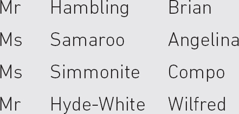
We should also test some invalid inputs, such as:
There are many more possibilities that infringe the rules in the specification, but these should serve to illustrate the point. You may be thinking that this simple specification could generate a very large number of test cases – and you would be absolutely right. One of our aims in using systematic test case design techniques will be to cut down the number of tests we need to run to achieve a given level of confidence in the software we are testing.
The test procedure needs to add some details along the following lines:
1. Select the <Name or Personal Details> option from the main menu.
2. Select the ‘input’ option from the <Name or Personal Details> menu.
3. Select ‘Mr’ from the ‘Title’ drop-down menu.
4. Check that the cursor moves to the ‘surname’ field.
5. Type in ‘Hambling’ and press the tab key once; check that the cursor moves to the ‘first name’ field.
6. Type in ‘Brian’ and press the Enter key.
7. Check that the Job Input screen is displayed.
8. . . .
That should be enough to demonstrate what needs to be defined, and also how slow and tedious such a test is to run, and we have only completed one of the test cases so far!
The test procedure collects together all the test cases related to this specification element so that they can all be executed together as a block; there would be several to test valid and non-valid inputs, as you have seen in the example.
In the wider test process, we move on to the test execution step next. In preparation for execution, the test execution schedule collects together all the tests and sequences them, considering any priorities (highest priority tests are run first) and any dependencies between tests. For example, it makes sense to do all the tests on the input screen together and to do all the tests that use input data afterwards; that way we get the input screen tests to do the data entry that we will need for the later tests. There might also be technical reasons why we run tests in a particular sequence; for example, a test of the password security needs to be done at the beginning of a sequence of tests because we need to be able to get into the system to run the other tests.
THE IDEA OF TEST COVERAGE
Test coverage is a very important idea because it provides a quantitative assessment of the extent and quality of testing. In other words, it answers the question ‘How much testing have you done?’ in a way that is not open to interpretation. Statements such as ‘I’m nearly finished’, or ‘I’ve done two weeks’ testing’ or ‘I’ve done everything in the test plan’ generate more questions than they answer. They are statements about how much testing has been done or how much effort has been applied to testing, rather than statements about how effective the testing has been or what has been achieved. We need to know about test coverage for two very important reasons:
• It provides a quantitative measure of the quality of the testing that has been done by measuring what has been achieved.
• It provides a way of estimating how much more testing needs to be done. Using quantitative measures, we can set targets for test coverage and measure progress against them.
Statements like ‘I have tested 75 per cent of the decisions’ or ‘I’ve tested 80 per cent of the requirements’ provide useful information. They are neither subjective nor qualitative; they provide a real measure of what has actually been tested. If we apply coverage measures to testing based on priorities, which are themselves based on the risks addressed by individual tests, we will have a reliable, objective and quantified framework for testing.
Test coverage can be applied to any systematic technique; in this chapter we will apply it to specification-based techniques to measure how much of the functionality has been tested, and to structure-based techniques to measure how much of the code has been tested. Coverage measures may be part of the completion criteria defined in the test plan (step 1 of a generalised test process) and used to determine when to stop testing in the final step of this process.
CHECK OF UNDERSTANDING
1. What defines the process of test execution?
2. Briefly compare a test case and a test condition.
3. Which document identifies the sequence in which tests are executed?
4. Describe the purpose of a test coverage measure.
CATEGORIES OF TEST CASE DESIGN TECHNIQUES
There are very many ways to design test cases. Some are general, others are very specific. Some are very simple to implement, others are difficult and complex to implement. The many excellent books published on software testing techniques every year testify to the rate of development of new and interesting approaches to the challenges that confront the professional software tester.
There is, however, a collection of test case design techniques that has come to be recognised as the most important ones for a tester to learn to apply, and these have been selected as the representatives of test case design for the Foundation Certificate, and hence for this book.
The test case design techniques we will look at are grouped into three categories:
• Those based on deriving test cases directly from a specification or a model of a system or proposed system, known as black-box techniques. So black-box techniques are based on an analysis of the test basis documentation, including both functional and non-functional aspects. They do not use any information regarding the internal structure of the component or system under test.
• Those based on deriving test cases directly from the structure of a component or system are known as white-box techniques. We will briefly introduce this category, which concentrates on tests based on the code written to implement a component or system in this chapter, but other aspects of structure, such as a menu structure, can be tested in a similar way. An optional section of the chapter provides a more in-depth treatment of these techniques.
• Those based on deriving test cases from the tester’s experience of similar systems and general experience of testing, known as experience-based techniques.
It is convenient to categorise techniques for test case design in this way (it is easier for you to remember, for one thing) but do not assume that these are the only categories or the only techniques; there are many more that can be added to the tester’s ‘tool kit’ over time.
The category known as ‘black-box’ techniques is so-called because the techniques in it take a view of the system that does not need to know what is going on ‘inside the box’. Some will recognise ‘black box’ as the name of anything technical that you can use but about which you know nothing or next to nothing. The natural alternative to ‘black box’ is ‘white box’ and so ‘white-box’ techniques are those that are based on internal structure rather than external function.
Experience-based testing was not really treated as ‘proper’ testing in testing prehistory, so it was given disdainful names such as ‘ad hoc’; the implication that this was not a systematic approach was enough to exclude it from many discussions about testing. Both the intellectual climate and the sophistication of experience-based techniques have moved on from those early days. It is worth bearing in mind that many systems are still tested in an experience-based way, partly because the systems are not specified in enough detail or in a sufficiently structured way to enable other categories of technique to be applied, or because neither the development team nor the testing team have been trained in the use of specification-based or structure-based techniques.
Before we look at these categories in detail, think for a moment about what we are trying to achieve. We want to try to check that a system does everything that its specification says it should do and nothing else. In practice, the ‘nothing else’ is the hardest part and generates the most tests; that is because there are far more ways of getting something wrong than there are ways of getting it right. Even if we just concentrate on testing that the system does what it is supposed to do, we will still generate a very large number of tests. This will be expensive and time-consuming, which means it probably will not happen, so we need to ensure that our testing is as efficient as possible. As you will see, the best techniques do this by creating the smallest set of tests that will achieve a given objective, and they do that by taking advantage of certain things we have learned about testing; for example, that defects tend to cluster in interesting ways.
Bear this in mind as we take a closer look at the categories of test case design techniques.
CHOOSING TEST TECHNIQUES
The decision of which test technique to use is not a simple one. There are many factors to bear in mind, some of which are listed in the box.
KEY SELECTION FACTORS
• Type of system or component that we are testing; for example it may be a database or a system to control a manufacturing process.
• Any regulatory standards that may apply. These may be related to the type of system; for example safety critical, the type of industry in which the system will be used; for example railway systems, or other regulated applications.
• Customer or contractual requirements. Some customers may demand more rigorous testing than others and this will likely be identified in any contract for purchase of the system.
• Level of risk. Risk may be defined rigorously, as in safety-critical systems, or more colloquially; for example relating to business risk.
• Type of risk. Commercial risk and risk to human safety are examples of different types of risk.
• Test objectives, which will define, formally or informally, how much and what kind of testing is needed.
• Documentation available as a test basis.
• Knowledge of the testers, which will determine what kinds of testing can be designed and implemented.
• Time and budget. Both set limits on how much testing can be done.
• Development life cycle, which may define specific testing stages, as in the V model (see Chapter 2), or testing may be an implicit part of development, as in Agile development.
• Use case models. Use case models identify how a system is expected to function from a user perspective, so the use case model will effectively determine the scope and level of testing.
• Experience of the type of defects found in similar systems, which may enable better informed testing that focuses on problem areas.
One or more of these factors may be important on any given occasion. Some leave no room for selection: regulatory or contractual requirements leave the tester with no choice. Test objectives, where they relate to exit criteria such as test coverage, may also lead to mandatory techniques. Where documentation is not available, or where time and budget are limited, the use of experience-based techniques may be favoured. All others provide pointers within a broad framework: level and type of risk will push the tester towards a particular approach, where high risk is a good reason for using systematic techniques; knowledge of testers, especially where this is limited, may narrow down the available choices; the type of system and the development life cycle will encourage testers to lean in one direction or another depending on their own particular experience. There are few clear-cut cases, and the exercise of sound judgement in selecting appropriate techniques is a mark of a good test manager or team leader.
BLACK-BOX TEST TECHNIQUES
The main thing about black-box test techniques is that they derive test cases directly from the specification or from some other kind of model of what the system should do. The source of information on which to base testing is known as the ‘test basis’. If a test basis is well defined and adequately structured, we can easily identify test conditions from which test cases can be derived.
The most important point about black-box test techniques is that specifications or models do not (and should not) define how a system should achieve the specified behaviour when it is built; it is a specification of the required (or at least desired) behaviour. One of the hard lessons that software engineers have learned from experience is that it is important to separate the definition of what a system should do (a specification) from the definition of how it should work (a design). This separation allows the two specialist groups (testers for specifications and designers for design) to work independently so that we can later check that they have arrived at the same place; that is, they have together built a system and tested that it works according to its specification.
If we set up test cases so that we check that desired behaviour actually occurs, then we are acting independently of the developers. If they have misunderstood the specification or chosen to change it in some way without telling anyone then their implementation will deliver behaviour that is different from what the model or specification said the system behaviour should be. Our test, based solely on the specification, will therefore fail and we will have uncovered a problem.
Bear in mind that not all systems are defined by a detailed formal specification. In some cases, the model we use may be quite informal. If there is no specification at all, the tester may have to build a model of the proposed system, perhaps by interviewing key stakeholders to understand what their expectations are. However formal or informal the model is, and however it is built, it provides a test basis from which we can generate tests systematically.
Remember, also, that the specification can contain non-functional elements as well as functions; topics such as reliability, usability and performance are examples. These need to be systematically tested as well.
What we need, then, are techniques that can explore the specified behaviour systematically and thoroughly in a way that is as efficient as we can make it. In addition, we use what we know about software to ‘home in’ on problems; each of the test case design techniques is based on some simple principles that arise from what we know in general about software behaviour.
You need to know five specification-based techniques for the Foundation Certificate:
• boundary value analysis;
• decision table testing;
• state transition testing;
• use case testing.
You should be capable of generating test cases for the first four of these techniques.
CHECK OF UNDERSTANDING
1. What do we call the category of test case design techniques that requires knowledge of how the system under test actually works?
2. What do black-box techniques derive their test cases from?
3. How do we make specification-based testing work when there is no specification?
Equivalence partitioning
Input partitions
Equivalence partitioning is based on a very simple idea: it is that in many cases the inputs to a program can be ‘chunked’ into groups of similar inputs. For example, a program that accepts integer values can accept as valid any input that is an integer (i.e. a whole number) and should reject anything else (such as a real number or a character). The range of integers is infinite, though the computer will limit this to some finite value in both the negative and positive directions (simply because it can only handle numbers of a certain size; it is a finite machine). Let us suppose, for the sake of an example, that the program accepts any value between −10,000 and +10,000 (computers actually represent numbers in binary form, which makes the numbers look much less like the ones we are familiar with, but we will stick to a familiar representation). If we imagine a program that separates numbers into two groups according to whether they are positive or negative, the total range of integers could be split into three ‘partitions’: the values that are less than zero; zero; and the values that are greater than zero. Each of these is known as an ‘equivalence partition’ because every value inside the partition is exactly equivalent to any other value as far as our program is concerned. So, if the computer accepts −2,905 as a valid negative integer we expect it also to accept −3. Similarly, if it accepts 100 it should also accept 2,345 as a positive integer. Note that we are treating zero as a special case. We could, if we chose to, include zero with the positive integers, but my rudimentary specification did not specify that clearly, so it is really left as an undefined value (and it is not untypical to find such ambiguities or undefined areas in specifications). It often suits us to treat zero as a special case for testing where ranges of numbers are involved; we treat it as an equivalence partition with only one member. So, we have three valid equivalence partitions in this case.
The equivalence partitioning technique takes advantage of the properties of equivalence partitions to reduce the number of test cases we need to write. Since all the values in an equivalence partition are handled in exactly the same way by a given program, we need only test one of them as a representative of the partition. In the example given, then, we need any positive integer, any negative integer and zero. We generally select values somewhere near the middle of each partition, so we might choose, say, −5,000; 0; and 5,000 as our representatives. These three test inputs exercise all three partitions and the theory tells us that if the program treats these three values correctly, it is very likely to treat all of the other values, all 19,998 of them in this case, correctly.
The partitions we have identified so far are called valid equivalence partitions because they partition the collection of valid inputs, but there are other possible inputs to this program that are not valid – real numbers, for example. We also have two input partitions of integers that are not valid: integers less than –10,000 and integers greater than 10,000. We should test that the program does not accept these, which is just as important as the program accepting valid inputs.
If you think about the example we have been using, you will soon recognise that there are far more possible non-valid inputs than valid ones, since all the real numbers (e.g. numbers containing decimals) and all characters are non-valid in this case. It is generally the case that there are far more ways to provide incorrect input than there are to provide correct input; as a result, we need to ensure that we have tested the program against the possible non-valid inputs. Here again, equivalence partitioning comes to our aid: all real numbers are equally non-valid, as are all alphabetic characters. These represent two non-valid partitions that we should test, using values such as 9.45 and ‘r’ respectively. There will be many other possible non-valid input partitions, so we may have to limit the test cases to the ones that are most likely to crop up in a real situation.
EXAMPLE EQUIVALENCE PARTITIONS
• valid input: integers in the range 100 to 999;
• valid partition: 100 to 999 inclusive;
• non-valid partitions: less than 100, more than 999, real (decimal) numbers and non-numeric characters;
• valid input: names with up to 20 alphabetic characters;
• valid partition: strings of up to 20 alphabetic characters;
• non-valid partitions: strings of more than 20 alphabetic characters, strings containing non-alphabetic characters.
Exercise 4.1
Suppose you have a bank account that offers variable interest rates: 0.5 per cent for the first £1,000 credit; 1 per cent for the next £1,000; 1.5 per cent for the rest. If you wanted to check that the bank was handling your account correctly, what valid input partitions might you use?
The answer can be found at the end of the chapter.
Output partitions
Just as the input to a program can be partitioned, so can the output. The program in the exercise above could produce outputs of 0.5 per cent, 1 per cent and 1.5 per cent, so we can use test cases that generate each of these outputs as an alternative to generating input partitions. An input value in the range £0.00–£1,000.00 generates the 0.5 per cent output; a value in the range £1,001.00–£2,000.00 generates the 1 per cent output; a value greater than £2,000.00 generates the 1.5 per cent output.
Other partitions
If we know enough about an application, we may be able to partition other values instead of or as well as input and output. For example, if a program handles input requests by placing them on one of a number of queues we could, in principle, check that requests end up on the right queue. In this case, a stream of inputs can be partitioned according to the queue we anticipate it will be placed into. This is more technical and difficult than input or output partitioning, but it is an option that can be considered when appropriate.
PARTITIONS – EXAMPLE 4.1
A mail-order company charges £2.95 postage for deliveries if the package weighs less than 2 kg, £3.95 if the package weighs 2 kg or more but less than 5 kg, and £5 for packages weighing 5 kg or more. Generate a set of valid test cases using equivalence partitioning.
The valid input partitions are: under 2 kg; 2 kg or over but less than 5 kg; and 5 kg or over.
Input values could be 1 kg, 3.5 kg, 7.5 kg. These produce expected results of £2.95, £3.95 and £5 respectively.
In this case there are no non-valid inputs (unless the scales fail).
Exercise 4.2
A mail-order company selling flower seeds charges £3.95 for postage and packing on all orders up to £20 value and £4.95 for orders above £20 value and up to £40 value. For orders above £40 value, there is no charge for postage and packing.
If you were using equivalence partitioning to prepare test cases for the postage and packing charges what valid partitions would you define?
What about non-valid partitions?
The answer can be found at the end of the chapter.
Boundary value analysis
One thing we know about the kinds of mistakes that programmers make is that errors tend to cluster around boundaries. For example, if a program should accept a sequence of numbers between 1 and 10, the most likely fault will be that values just outside this range are incorrectly accepted or that values just inside the range are incorrectly rejected. In the programming world, these faults coincide with particular programming structures such as the number of times a program loop is executed or the exact point at which a loop should stop executing.
This works well with our equivalence partitioning idea because partitions must have boundaries. (Where partitions do not have boundaries, for example in the set of days of the week, the boundary analysis technique cannot be used.) A partition of integers between 1 and 99, for instance, has a lowest value, 1, and a highest value, 99. These are called boundary values. Actually, they are called valid boundary values because they are the boundaries on the inside of a valid partition. What about the values on the outside? Yes, they have boundaries too. So, the boundary of the non-valid values at the lower end will be zero because it is the first value you come to when you step outside the partition at the bottom end. (You can also think of this as the highest value inside the non-valid partition of integers that are less than one, of course.) At the top end of the range we also have a non-valid boundary value, 100.
This is the boundary value technique, more or less. For most practical purposes the boundary value analysis technique needs to identify just two values at each boundary. For reasons that need not detain us here there is an alternative version of the technique that uses three values at each boundary. For this variant, which is the one documented in BS 7925-2, we include one more value at each boundary when we use boundary value analysis: the rule is that we use the boundary value itself and one value (as close as you can get) either side of the boundary.
So, in this case lower boundary values will be 0, 1, 2 and upper boundary values will be 98, 99, 100. What does ‘as close as we can get’ mean? It means take the next value in sequence using the precision that has been applied to the partition. If the numbers are to a precision of 0.01, for example, the lower boundary values are 0.99, 1.00, 1.01 and the upper boundary values are 98.99, 99.00, 99.01.
When you come to take your exam, you will find that the exam recognises that there are two possible approaches to boundary value analysis. For this reason, any questions about boundary value analysis will clearly signal whether you are expected to identify two or three values at any boundary. You will find that this causes no problems, but there are examples below using both the two value and the three value approach, just to be on the safe side, to ensure that you do not get taken by surprise in the exam.
The best way to consolidate the idea of boundaries is to look at some examples.
• The boiling point of water – the boundary is at 100 degrees Celsius, so for the three value boundary approach, the boundary values will be 99 degrees, 100 degrees, 101 degrees – unless you have a very accurate digital thermometer, in which case they could be 99.9 degrees, 100.0 degrees, 100.1 degrees. For the two value approach the corresponding values are 100 and 101.
• Exam pass – if an exam has a pass boundary at 40 per cent, merit at 60 per cent and distinction at 80 per cent the three value boundaries are 39, 40, 41 for pass, 59, 60, 61 for merit, 79, 80, 81 for distinction. It is unlikely that marks would be recorded at any greater precision than whole numbers. The two value equivalents are 39 and 40, 59 and 60, and 79 and 80 respectively.
Exercise 4.3
A system is designed to accept scores from independent markers who have marked the same examination script. Each script should have five individual marks, each of which is out of 20, and a total for the script. Two markers’ scores are compared and differences greater than three in any question score or 10 overall are flagged for further examination.
Using equivalence partitioning and boundary value analysis, identify the boundary values that you would explore for this scenario.
(In practice, some of the boundary values might actually be in other equivalence partitions, and we do not need to test them twice, so the total number of boundary values requiring testing might be less than you might expect.) The answer can be found at the end of the chapter.
CHECK OF UNDERSTANDING
1. What is the relationship between a partition and a boundary?
2. Why are equivalence partitioning and boundary value analysis often used together?
3. Explain what is meant by ‘as close as possible to a boundary’?
Decision table testing
Specifications often contain business rules to define the functions of the system and the conditions under which each function operates. Individual decisions are usually simple, but the overall effect of these logical conditions can become quite complex. As testers we need to be able to assure ourselves that every combination of these conditions that might occur has been tested, so we need to capture all the decisions in a way that enables us to explore their combinations. The mechanism usually used to capture the logical decisions is called a decision table.
A decision table lists all the input conditions that can occur and all the actions that can arise from them. These are structured into a table as rows, with the conditions at the top of the table and the possible actions at the bottom. Business rules, which involve combinations of conditions to produce some combination of actions, are arranged across the top. Each column therefore represents a single business rule (or just ‘rule’) and shows how input conditions combine to produce actions. Thus, each column represents a possible test case, since it identifies both inputs and expected outputs. This is shown schematically in the box below.
DECISION TABLE STRUCTURE

Business rule 1 requires all conditions to be true to generate action 1. Business rule 2 results in action 2 if condition 1 is false and condition 2 is true, but does not depend on condition 3. Business rule 3 requires conditions 1 and 2 to be true and condition 3 to be false.
In reality the number of conditions and actions can be quite large, but usually the number of combinations producing specific actions is relatively small. For this reason, we do not enter every possible combination of conditions into our decision table but restrict it to those combinations that correspond to business rules – this is called a limited entry decision table to distinguish it from a decision table with all combinations of inputs identified. In this chapter we will always mean the limited entry kind when we refer to a decision table.
As usual, we use an example to clarify what we mean.
DECISION TABLE TESTING – EXAMPLE 4.3
A supermarket has a loyalty scheme that is offered to all customers. Loyalty cardholders enjoy the benefits of either additional discounts on all purchases (rule 3) or the acquisition of loyalty points (rule 4), which can be converted into vouchers for the supermarket or to equivalent points in schemes run by partners. Customers without a loyalty card receive an additional discount only if they spend more than £100 on any one visit to the store (rule 2), otherwise only the special offers offered to all customers apply (rule 1).

From the decision table, we can determine test cases by setting values for the conditions and determining the expected output; for example, from rule 1 we could input a normal customer with a £50 transaction and check that no discount was applied. The same customer with a £150 transaction (rule 2) should attract a discount. Thus, we can see that each column of the decision table represents a possible test case.
CHECK OF UNDERSTANDING
1. What is a decision table derived from?
2. Why does decision table testing use limited entry decision tables?
3. Describe how test cases are identified from decision tables.
4. Which element of a decision table defines the expected output for a test case?
Exercise 4.4
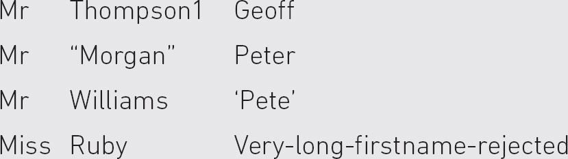
A mutual insurance company has decided to float its shares on the stock exchange and is offering its members rewards for their past custom at the time of flotation. Anyone with a current policy will benefit provided it is a ‘with-profits’ policy and they have held it since 2001. Those who meet these criteria can opt for either a cash payment or an allocation of shares in the new company; those who have held a qualifying policy for less than the required time will be eligible for a cash payment but not for shares. Here is a decision table reflecting those rules.
What result would you expect to get for the following test case?
Billy Bunter is a current policy holder who has held a ‘with-profits’ policy since 2003.
The answer can be found at the end of the chapter.
State transition testing
The previous technique, decision table testing, is particularly useful in systems where combinations of input conditions produce various actions. Now we consider a similar technique, but this time we are concerned with systems in which outputs are triggered by changes to the input conditions, or changes of ‘state’; in other words, behaviour depends on current state and past state, and it is the transitions that trigger system behaviour. It will be no surprise to learn that this technique is known as state transition testing or that the main diagram used in the technique is called a state transition diagram.
Look at the box to see an example of a state transition diagram.
A state transition diagram is a representation of the behaviour of a system. It is made up from just two symbols.
which is the symbol for a state. A state is just what it says it is: the system is ‘static’, in a stable condition from which it will only change if it is stimulated by an event of some kind. For example, a TV stays ‘on’ unless you turn it ‘off’; a multifunction watch tells the time unless you change mode. The second is
![]()
which is the symbol for a transition; that is, a change from one state to another. The state change will be triggered by an event (e.g. pressing a button or switching a switch). The transition will be labelled with the event that caused it and any action that arises from it. So, we might have ‘mode button pressed’ as an event and ‘presentation changes’ as the action. Usually (but not necessarily) the start state will have a double arrowhead pointing to it. Often the start state is obvious anyway.
If we have a state transition diagram representation of a system, we can analyse the behaviour in terms of what happens when a transition occurs.
Transitions are caused by events and they may generate outputs and/or changes of state. An event is anything that acts as a trigger for a change; it could be an input to the system, or it could be something inside the system that changes for some reason, such as a database field being updated.
In some cases, an event generates an output; in others, the event changes the system’s internal state without generating an output; and in still others, an event may cause an output and a change of state. What happens for each change is always deducible from the state transition diagram.
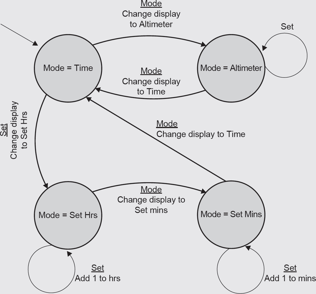
STATE TRANSITION DIAGRAM – EXAMPLE 4.4
A hill-walker’s watch has two modes: Time and Altimeter. In Time mode, pressing the Mode switch causes the watch to switch to Alt mode; pressing Mode again returns to Time mode. While the watch is in Alt mode the Set button has no effect.
When the watch is in Time mode pressing the Set button transitions the watch into Set Hrs, from which the Hrs display can be incremented by pressing the Set button. If the Mode switch is pressed while the watch is in Set Hrs mode the watch transitions to Set Mins mode, in which pressing the Set button increments the Mins display. If the Mode button is pressed in this mode, the watch transitions back to Time mode (Figure 4.1).
Note that not all events have an effect in all states. Where an event does not have an effect on a given state it is usually omitted, but it can be shown as an arrow starting from the state and returning to the same state to indicate that no transition takes place; this is sometimes known as a ‘null’ transition or an ‘invalid’ transition.
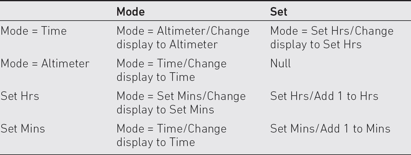
Rather than work out what happens for each event each time we want to initiate a test, we can take the intermediate step of creating what is known as a state table (ST). An ST records all the possible events and all the possible states; for each combination of event and state it shows the outcome in terms of the new state and any outputs that are generated.
The ST is the source from which we usually derive test cases. It makes sense to do it this way because the analysis of state transitions takes time and can be a source of errors; it is better to do this task once and then have a simple way of generating tests from it than to do it every time we want to generate a new test case.
Table 4.1 provides an example of what an ST looks like.
Figure 4.1 State transition diagram of the hill-walker’s watch
An ST has a row for each state in the state transition diagram and a column for every event. For a given row and column intersection, we read off the state from the state transition diagram and note what effect (if any) each event has. If the event has no effect, we label the table entry with a symbol that indicates that nothing happens; this is sometimes called a ‘null’ transition or an ‘invalid’ transition. If the event does have an effect, label the table entry with the state to which the system transitions when the given event occurs; if there is also an output (there is sometimes but not always) the output is indicated in the same table entry separated from the new state by the ‘/’ symbol. The example shown in Table 4.1 is the ST for Figure 4.1, which we drew in the previous box.
Table 4.1 ST for the hill-walker’s watch
Once we have an ST it is a simple exercise to generate the test cases that we need to exercise the functionality by triggering state changes.
STATE TRANSITION TESTING – EXAMPLE 4.4
We generate test cases by stepping through the ST. If we begin in Time mode, then the first test case might be to press Mode and observe that the watch changes to Alt state; pressing Mode again becomes test case 2, which returns the watch to Time state. Test case 3 could press Set and observe the change to Set Hrs mode and then try a number of presses of Set to check that the incrementing mechanism works. In this way we can work our way systematically round the ST until every single transition has been exercised. If we want to be more sophisticated, we can exercise pairs of transitions; for example, pressing Set twice as a single test case to check that Hrs increments correctly. We should also test all the negative cases; that is, those cases where the ST indicates there is no valid transition.
1. What is the main use of an ST for testers?
2. Name three components of a state transition diagram.
3. How are negative tests identified from an ST?
4. What is meant by the term ‘invalid’ transition?
Exercise 4.5
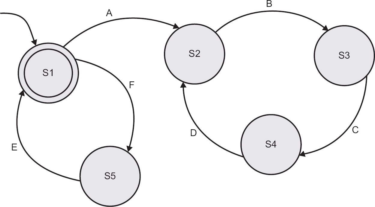
In the state transition diagram in Figure 4.2, which of the sequences of transitions below is valid?
a. ABCDE
b. FEABC
c. ABCEF
d. EFADC
The answer can be found at the end of the chapter.
Figure 4.2 State transition diagram
Use case testing
Use cases are one way of specifying functionality as business scenarios or process flows. They capture the individual interactions between ‘actors’ and the system. An actor represents a particular type of user and the use cases capture the interactions that each user takes part in to produce some output that is of value. Test cases based on use cases at the business process level, often called scenarios, are particularly useful in exercising business rules or process flows and will often identify gaps or weaknesses in these that would not be found by exercising individual components in isolation. This makes use case testing very effective in defining acceptance tests because the use cases represent actual likely use.
Use cases may also be defined at the system level, with preconditions that define the state the system needs to be in on entry to a use case to enable the use case to complete successfully, and postconditions that define the state of the system on completion of the use case. Use cases typically have a mainstream path, defining the expected behaviour, and one or more alternative paths related to such aspects as error conditions. Well-defined use cases can therefore be an excellent basis for system level testing, and they can also help to uncover integration defects caused by incorrect interaction or communication between components.
In practice, writing a test case to represent each use case is often a good starting point for testing, and use case testing can be combined with other specification-based testing.
USE CASES
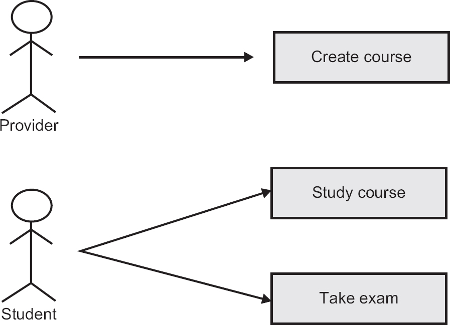
In a use case diagram (e.g. Figure 4.3), each type of user is known as an actor and an actor stands for all users of the type. Use cases are activities carried out for that actor by the system. This is, in effect, a high-level view of requirements.
The diagram alone does not provide enough detail for testing, so we need some textual description of the processes involved as well.
Use case testing has the major benefit that it relates to real user processes, so it offers an opportunity to exercise a complete process flow. The principles applied elsewhere can be applied here: first, test the highest priority (highest value) use cases by taking typical examples; then exercise some attempts at incorrect process flows; and then exercise the boundaries.
CHECK OF UNDERSTANDING
1. What is the purpose of a use case?
2. What is the relationship between a use case and a test case?
3. Briefly compare equivalence partitioning and use case testing.
WHITE-BOX TEST TECHNIQUES
White-box test techniques are used to explore system or component structures at several levels. At the component level, the structures of interest will be program structures such as program statements and decisions; at the integration level, we may be interested in exploring the way components interact with other components (in what is usually termed a calling structure); at the system level, we may be interested in how users will interact with a menu structure. All these are examples of structures and all may be tested using white-box test techniques.
Instead of exercising a component or system to see if it functions correctly, using a specification or model of the system to determine correct functioning, white-box tests focus on ensuring that elements of the structure of a component, sub-system or system are correctly exercised. For example, we can use white-box test techniques to ensure that each statement in the code of a component is executed at least once, using a technique called statement testing; we can test that each decision in a component is exercised and behaves as expected; we can test that components interact correctly in a sub-system; we can test that user interaction with menus is correct.
We will focus here on statement testing and decision testing, both of which are usually deployed at the component or program level.
Statement testing and coverage
Statement testing exercises the executable statements in the code. Tests are designed to attempt to force the program to execute particular statements by setting a program to a known start state and inputting data that will cause the required statements to be executed. The expected outputs of the test will also be predicted from the program code so that, on completion of the test, it can be determined whether the test executed the required statements. An analyser tool can also be used to determine which statements were executed by a test run.
Statement coverage is measured as the number of statements executed by the tests divided by the total number of executable statements in the test object, normally expressed as a percentage. A target for statement coverage can be set and statement testing would continue until the required target statement coverage is achieved.
Decision testing and coverage
Decision testing exercises the decisions in the code. In a similar way to statement testing, tests are designed to attempt to force the program to execute particular decisions in particular ways. This will be achieved by setting the program to a known start state and inputting data that is expected to set given decisions so that the program exits them from the required exit (true or false). To do this, the test cases follow the control flows that occur from a decision point (e.g. for an IF statement, one for the true outcome and one for the false outcome; for a CASE statement, test cases are required for all the possible outcomes, including the default outcome). As with statement testing, the expected outputs of the test will also be predicted from the program code so that, on completion of the test, it can be determined whether the test executed the required decisions appropriately. An analyser tool can also be used to determine which decisions were executed by a test run.
Decision coverage is measured as the number of decision outcomes executed by the tests divided by the total number of decision outcomes in the test object, normally expressed as a percentage. A target for decision coverage can be set and decision testing would continue until the required target decision coverage is achieved.
The value of statement and decision testing
When 100 per cent statement coverage is achieved, it ensures that all executable statements in the code have been tested at least once, but it does not ensure that all decision logic has been tested. Of the two white-box techniques discussed in this syllabus, statement testing may provide less coverage than decision testing. To achieve 100 per cent decision coverage, all decision outcomes must be exercised, so for each decision, both the true outcome and the false outcome, even when there is no explicit false statement (e.g. in the case of an IF statement without an ELSE in the code), must be executed successfully.
Statement coverage can help to find defects in code that was not exercised by other tests. For example, a functional test may run and confirm the correct output, even though the program does not always process the inputs correctly. A functional test is limited to checking that a given input achieves the correct functional output, but it may be that it only exercises part of a program. A more thorough test of the program in isolation may discover that the program does not always behave exactly as expected, and this defect may have functional implications that were not discovered during black-box testing.
Similarly, decision testing may help to find defects in code where functional tests have not forced the program to take both true and false decision exits. Here again, a more thorough exploration of the decision structures in the code can unearth problems that could not easily be detected, or could not be detected at all, by black-box testing.
Achieving 100 per cent decision coverage guarantees that 100 per cent statement coverage has also been achieved, but the reverse is not necessarily true.
The following material is not examinable. Readers who wish to skip this material at first reading may resume the examinable material on page 145.
WHITE-BOX TESTING IN DETAIL
White-box test techniques are used to explore system or component structures at several levels. At the component level, the structures of interest are program structures such as decisions; at the integration level we may be interested in exploring the way components interact with other components (in what is usually termed a calling structure); at the system level, we may be interested in how users will interact with a menu structure. All these are examples of structures and all may be tested using white-box test case design techniques. Instead of exercising a component or system to see if it functions correctly, white-box tests focus on ensuring that particular elements of the structure itself are correctly exercised. For example, we can use structural testing techniques to ensure that each statement in the code of a component is executed at least once. At the component level, where white-box testing is most commonly used, the test case design techniques involve generating test cases from code, so we need to be able to read and analyse code. As you will see later, in Chapter 6, code analysis and white-box testing at the component level are mostly done by specialist tools, but a knowledge of the techniques is still valuable. You may wish to run simple test cases on code to ensure that it is basically sound before you begin detailed functional testing, or you may want to interpret test results from programmers to ensure that their testing adequately exercises the code.
The CTFL syllabus does not require this complete level of understanding and takes a simplified approach that uses simplified control flow graphs (introduced in the section on Simplified control flow graphs). The following paragraphs can therefore be considered optional for readers whose interest is solely to pass the CTFL exam at this stage but, for anyone intending to progress to the more advanced levels, they provide an essential introduction to code analysis that will be required for these exams and that will be needed in testing real software.
Our starting point, then, is the code itself. The best route to a full understanding of white-box techniques is to start here and work through the whole section.
READING AND INTERPRETING CODE
Often the term ‘code’ will be taken to mean pseudo code, and this is particularly relevant when addressing a non-specific audience or an international audience. Pseudo code is a much more limited language than any real programming language, but it enables designers to create all the main control structures needed by programs. It is sometimes used to document designs before they are coded into a programming language.
In the next few boxes we will introduce all the essential elements of pseudo code that you will need to be able to analyse code and create test cases.
Wherever you see the word ‘code’ from here on in this chapter, read it as ‘pseudo code’.
Real programming languages have a wide variety of forms and structures – so many that we could not adequately cover them all. The advantage of pseudo code in this respect is that it has a simple structure.
OVERALL PROGRAM STRUCTURE
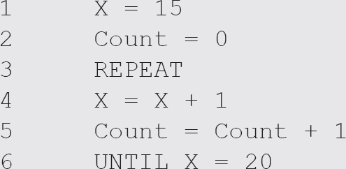
Code can be of two types: executable and non-executable. Executable code instructs the computer to take some action; non-executable code is used to prepare the computer to do its calculations, but it does not involve any actions. For example, reserving space to store a calculation (this is called a declaration statement) involves no actions. In pseudo code, non-executable statements will be at the beginning of the program; the start of the executable part is usually identified by BEGIN, and the end of the program by END. So, we get the following structure:
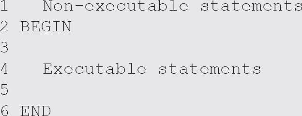
If we were counting executable statements, we would count lines 2, 4 and 6. Line 1 is not counted because it is non-executable. Lines 3 and 5 are ignored because they are blank.
If there are no non-executable statements there may be no BEGIN or END either, but there will always be something separating non-executable from executable statements where both are present.
Now we have a picture of an overall program structure we can look inside the code. Surprisingly, there are only three ways that executable code can be structured, so we only have three structures to learn. The first is simple and is known as sequence: that just means that the statements are exercised one after the other as they appear on the page. The second structure is called selection: in this case the computer has to decide if a condition (known as a Boolean condition) is true or false. If it is true the computer takes one route, and if it is false the computer takes a different route. Selection structures therefore involve decisions. The third structure is called iteration: it simply involves the computer exercising a chunk of code more than once; the number of times it exercises the chunk of code depends on the value of a condition (just as in the selection case). Let us look at that a little closer.
SEQUENCE
The following program is purely sequential:

The BEGIN and END have been omitted in this case, since there were no non-executable statements; this is not strictly correct but is common practice, so it is wise to be aware of it and remember to check whether there are any non-executable statements when you do see BEGIN and END in a program. The computer would execute those three statements in sequence, so it would read (input) a value into A (this is just a name for a storage location), then read another value into B, and finally add them together and put the answer into C.
SELECTION
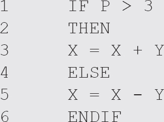
Here we ask the computer to evaluate the condition P > 3, which means compare the value that is in location P with 3. If the value in P is greater than 3, then the condition is true; if not, the condition is false. The computer then selects which statement to execute next. If the condition is true it will execute the part labelled THEN, so it executes line 3. If the condition is false, it will execute line 5. After it has executed either line 3 or line 5 it will go to line 6, which is the end of the selection (IF THEN ELSE) structure. From there, it will continue with the next line in sequence.
There may not always be an ELSE part, as below:
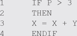
In this case the computer executes line 3 if the condition is true or moves on to line 4 (the next line in sequence) if the condition is false.
ITERATION
Iteration structures are called loops. The most common loop is known as a DO WHILE (or WHILE DO) loop and is illustrated below:

As with the selection structures, there is a decision. In this case the condition that is tested at the decision is X < 20. If the condition is true, the program ‘enters the loop’ by executing the code between DO and END DO. In this case the value of X is increased by one and the value of Count is increased by one. When this is done the program goes back to line 3 and repeats the test. If X < 20 is still true, the program ‘enters the loop’ again. This continues as long as the condition is true. If the condition is false, the program goes directly to line 6 and then continues to the next sequential instruction. In the program fragment above, the loop will be executed five times before the value of X reaches 20 and causes the loop to terminate. The value of Count will then be 5.
There is another variation of the loop structure known as a REPEAT UNTIL loop. It looks like this:
The difference from a DO WHILE loop is that the condition is at the end, so the loop will always be executed at least once. Every time the code inside the loop is executed, the program checks the condition. When the condition is true, the program continues with the next sequential instruction. The outcome of this REPEAT UNTIL loop will be exactly the same as the DO WHILE loop above.
CHECK OF UNDERSTANDING
1. What is meant by the term executable statement?
2. Briefly describe the two forms of looping structure introduced in this section.
3. What is a selection structure?
4. How many different paths are there through a selection structure?
Flow charts
Now that we can read code, we can go a step further and create a visual representation of the structure that is much easier to work with. The simplest visual structure to draw is the flow chart, which has only two symbols. Rectangles represent sequential statements and diamonds represent decisions. More than one sequential statement can be placed inside a single rectangle as long as there are no decisions in the sequence. Any decision is represented by a diamond, including those associated with loops.
Let us look at our earlier examples again.
To create a flow chart representation of a complete program, all we need to do is to connect together all the different bits of structure.
Figure 4.4 Flow chart for a sequential program
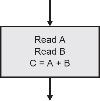
Figure 4.5 Flow chart for a selection (decision) structure

Figure 4.6 Flow chart for an iteration (loop) structure

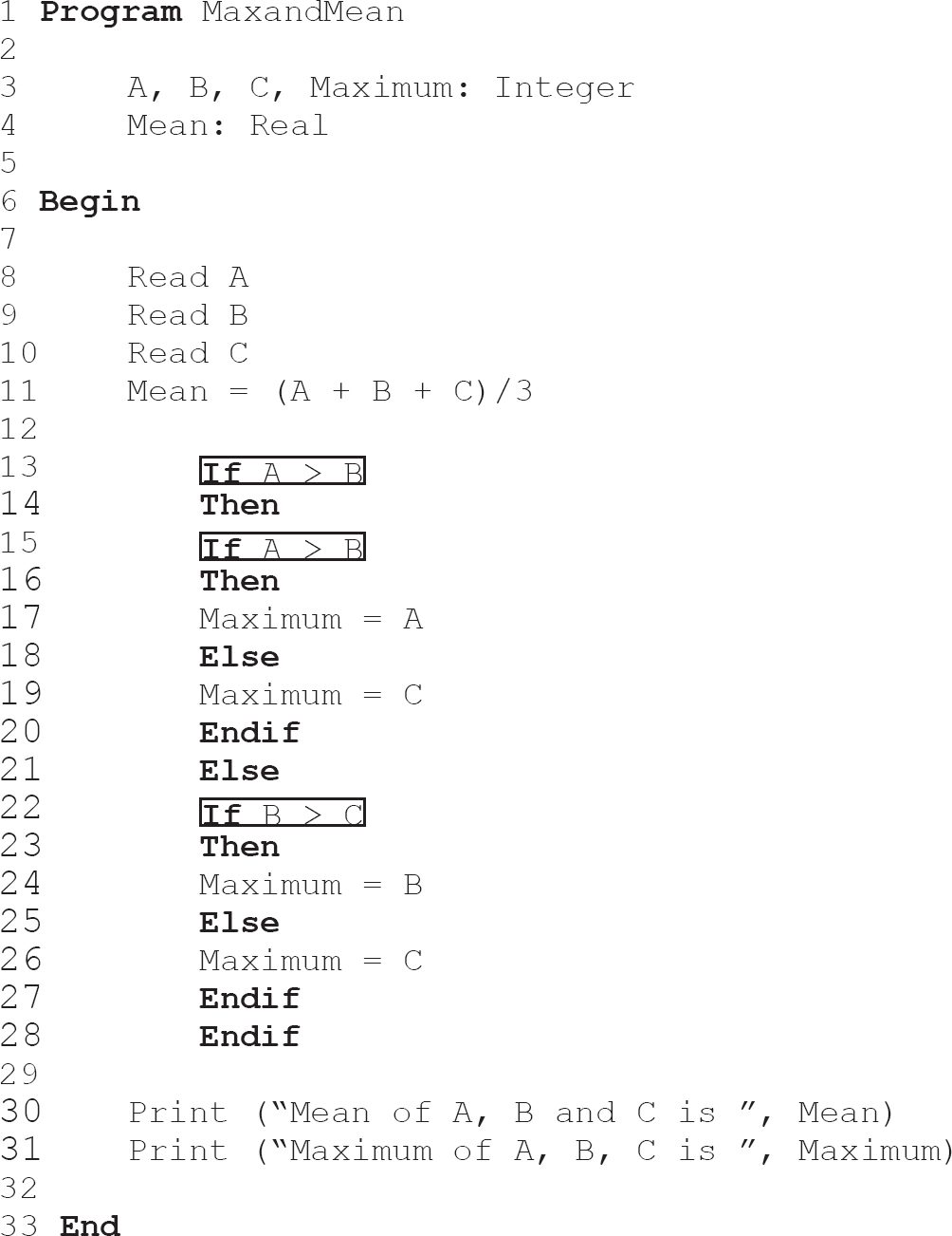
PROGRAM ANALYSIS – EXAMPLE 4.5
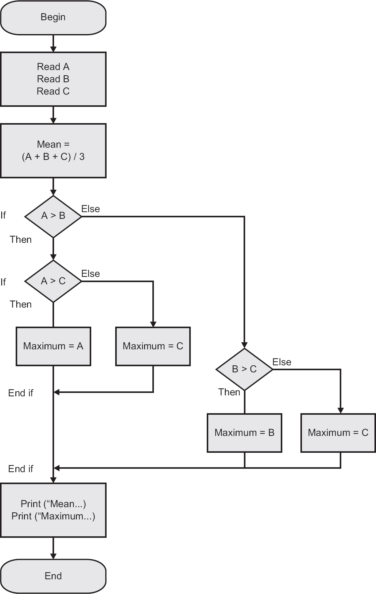
Here is a simple program for calculating the mean and maximum of three integers.

Note one important thing about this code: it has some non-executable statements (those before the Begin and those after the Begin that are actually blank lines) that we will have to take account of when we come to count the number of executable statements later. The line numbering makes it a little easier to do the counting.
By the way, you may have noticed that the program does not recognise if two of the numbers are the same value, but simplicity is more important than sophistication at this stage.
This program can be expressed as a flow chart; have a go at drawing it before you look at the solution in the text.
Figure 4.7 shows the flow chart for Example 4.5.
Figure 4.7 Flow chart representation for Example 4.5
Before we move on to look at how we generate test cases for code, we need to look briefly at another form of graphical representation called the control flow graph.
Control flow graphs
A control flow graph provides a method of representing the decision points and the flow of control within a piece of code, so it is just like a flow chart except that it only shows decisions. A control flow graph is produced by looking only at the statements affecting the flow of control.
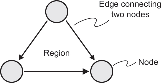
The graph itself is made up of two symbols: nodes and edges. A node represents any point where the flow of control can be modified (i.e. decision points), or the points where a control structure returns to the main flow (e.g. END WHILE or ENDIF). An edge is a line connecting any two nodes. The closed area contained within a collection of nodes and edges, as shown in the diagram, is known as a region.
We can draw ‘subgraphs’ to represent individual structures. For a flow graph the representation of sequence is just a straight line, since there is no decision to cause any branching.
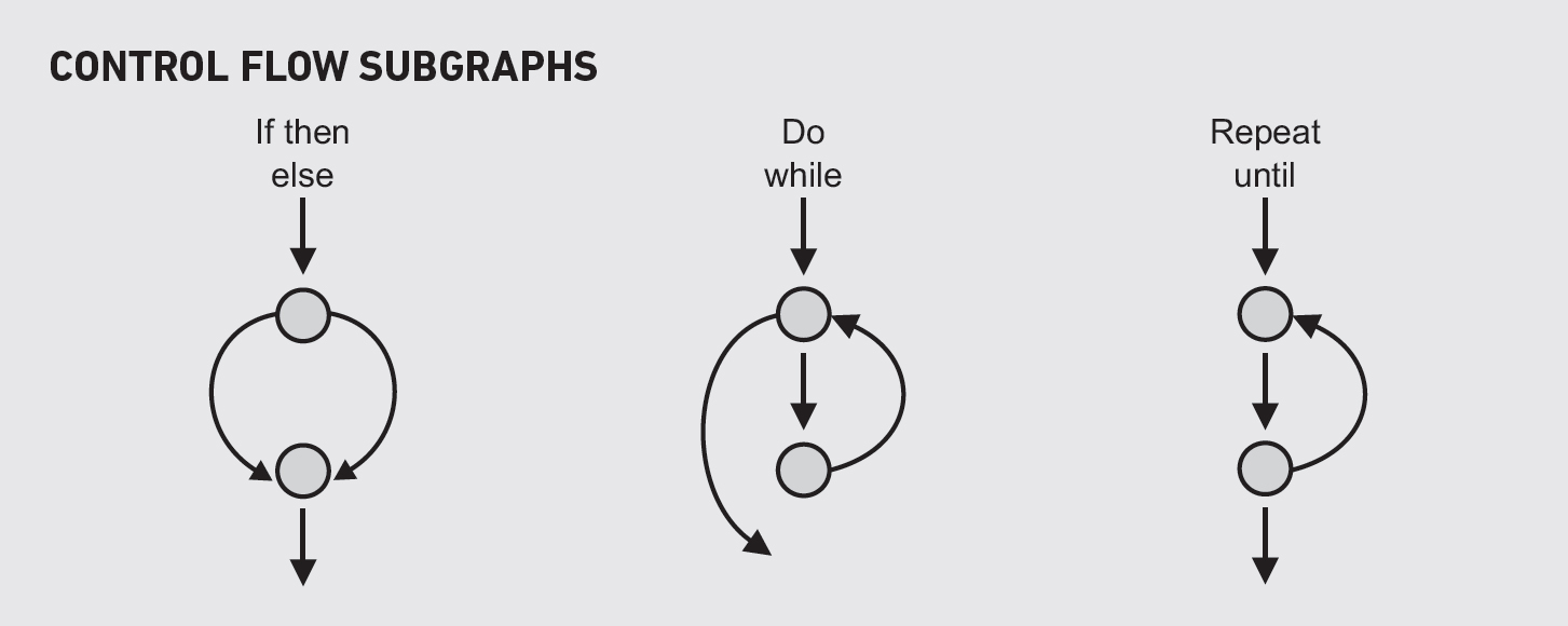
The subgraphs show what the control flow graph would look like for the program structures we are already familiar with.
Any chunk of code can be represented by using these subgraphs.
The steps are as follows:
1. Analyse the component to identify all control structures; that is, all statements that can modify the flow of control, ignoring all sequential statements.
2. Add a node for any decision statement.
3. Expand the node by substituting the appropriate subgraph representing the structure at the decision point.
As an example, we will return to Example 4.5.
Step 1 breaks the code into statements and identifies the control structures, ignoring the sequential statements, in order to identify the decision points; these are highlighted below.
Step 2 adds a node for each branching or decision statement (Figure 4.8).
Step 3 expands the nodes by substituting the appropriate subgraphs (Figure 4.9).
Figure 4.8 Control flow graph showing subgraphs as nodes

Figure 4.9 Control flow graph with subgraphs expanded

1. What is the difference between a flow chart and a control flow graph?
2. Name the three fundamental program structures that can be found in programs.
3. Briefly explain what is meant by an edge, a node and a region in a control flow graph.
Exercise 4.6
Draw a flow chart and a control flow graph to represent the following code:
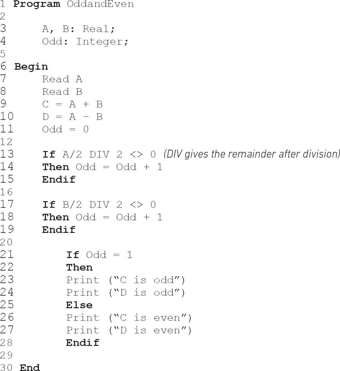
The answer can be found at the end of the chapter.
Statement testing and coverage
Statement testing is testing aimed at exercising programming statements. If we aim to test every executable statement, we call this full or 100 per cent statement coverage. If we exercise half the executable statements this is 50 per cent statement coverage, and so on. Remember: we are only interested in executable statements, so we do not count non-executable statements at all when we are measuring statement coverage.
Why measure statement coverage? It is a very basic measure that testing has been (relatively) thorough. After all, a suite of tests that had not exercised all of the code would not be considered complete. Actually, achieving 100 per cent statement coverage does not tell us very much, and there are much more rigorous coverage measures that we can apply, but it provides a baseline from which we can move on to more useful coverage measures. Look at the following pseudo code:
A flow chart can represent this, as in Figure 4.10.
Having explored flow charts and flow graphs a little, you will see that flow charts are very good at showing you where the executable statements are; they are all represented by diamonds or rectangles and where there is no rectangle, there is no executable code. A flow graph is less cluttered, showing only the structural details, in particular where the program branches and rejoins. Do we need both diagrams? Well, neither has everything that we need. However, we can produce a version of the flow graph that allows us to determine statement coverage.
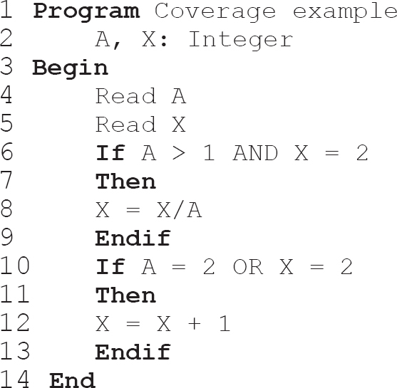
To do this we build a conventional control flow graph but then we add a node for every branch in which there are one or more statements. Take the Coverage example: we can produce its flow graph easily as shown in Figure 4.11.
Before we proceed, let us confirm what happens when a program runs. Once the program starts, it will run through to the end executing every statement that it comes to in sequence. Control structures will be the only diversion from this end-to-end sequence, so we need to understand what happens with the control structures when the program runs. The best way to do that is to ‘dry run’ the program with some inputs; this means writing down the inputs and then stepping through the program logic, noting what happens at each step and what values change. When you get to the end, you will know what the output values (if any) will be and you will know exactly what path the program has taken through the logic.
Figure 4.10 Flow chart for Coverage example
THE HYBRID FLOW GRAPH
Figure 4.11 The hybrid flow graph
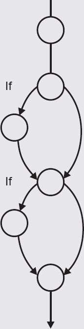
Note the additional nodes that represent the edges with executable statements in them; they make it a little easier to identify what needs to be counted for statement coverage.
Flow charts, control flow graphs and hybrid flow graphs all show essentially the same information, but sometimes one format is more helpful than another. We have identified the hybrid flow graph as a useful combination of the control flow graph and the control flow chart. To make it even more useful we can add to it labels to indicate the paths that a program can follow through the code. All we need to do is to label each edge; paths are then made up from sequences of the labels, such as abeh, which make up a path through the code (see Figure 4.12).
Figure 4.12 Paths through the hybrid flow graph example

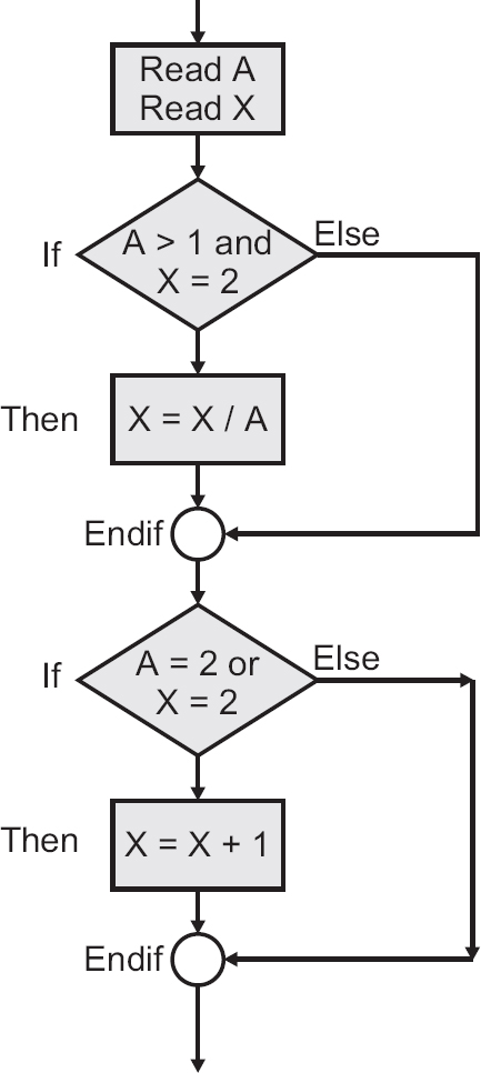
In the Coverage example, for which we drew the flow chart in Figure 4.10, 100 per cent statement coverage can be achieved by writing a single test case that follows the path acdfgh (using lower case letters to label the arcs on the diagram that represent path fragments). By setting A = 2 and X = 2 at point a, every statement will be executed once. However, what if the first decision should be an OR rather than an AND? The test would not have detected the error, since the condition will be true in both cases. Similarly, if the second decision should have stated X > 2, this error would have gone undetected because the value of A guarantees that the condition is true. Also, there is a path through the program in which X goes unchanged (the path abeh). If this were an error, it would also go undetected.
Remember that statement coverage takes into account only executable statements. There are 12 in the Coverage example if we count the BEGIN and END statements, so statement coverage would be 12/12 or 100 per cent. There are alternative ways to count executable statements: some people count the BEGIN and END statements; some count the lines containing IF, THEN and ELSE; some count none of these. It does not matter as long as:
• You exclude the non-executable statements that precede BEGIN.
• You ignore blank lines that have been inserted for clarity.
• You are consistent about what you do or do not include in the count with respect to control structures.
As a general rule, for the reasons given above, statement coverage is too weak to be considered an adequate measure of test effectiveness.
STATEMENT TESTING – EXAMPLE 4.6
Here is an example of the kind you might see in an exam. Try to answer the question, but if you get stuck the answer follows immediately in the text.
Here is a program. How many test cases will you need to achieve 100 per cent statement coverage and what will the test cases be?

Figure 4.13 shows what the flow graph looks like. It is drawn in the hybrid flow graph format so that you can see which branches need to be exercised for statement coverage.
Figure 4.13 Paths through the hybrid flow graph – Example 4.6

It is clear from the flow graph that the left-hand side (Balance below £1,000) need not be exercised, but there are two alternative paths (Balance between £1,000 and £10,000 and Balance > £10,000) that need to be exercised.
So, we need two test cases for 100 per cent statement coverage and Balance = £5,000, Balance = £20,000 will be suitable test cases.
Alternatively, we can aim to follow the paths abcegh and abdfgh marked on the flow graph. How many test cases do we need to do that?
We can do this with one test case to set the initial balance value to a value between £1,000 and £10,000 (to follow abcegh) and one test case to set the initial balance to something higher than £10,000, say £12,000 (to follow path abdfgh).
So, we need two test cases to achieve 100 per cent statement coverage in this case.
Now look at this example from the perspective of the tester actually trying to achieve statement coverage. Suppose we have set ourselves an exit criterion of 100 per cent statement coverage by the end of component testing. If we ran a single test with an input of Balance = £10,000 we can see that that test case would take us down the path abdfgh, but it would not take us down the path abcegh, and line 14 of the pseudo code would not be exercised. So that test case has not achieved 100 per cent statement coverage and we will need another test case to exercise line 14 by taking path abcegh. We know that Balance = £5,000 would do that. We can build up a test suite in this way to achieve any desired level of statement coverage.
1. What is meant by statement coverage?
2. In a flow chart, how do you decide which paths to include in determining how many test cases are needed to achieve a given level of statement coverage?
3. Does 100 per cent statement coverage exercise all the paths through a program?
Exercise 4.7
For the following program:
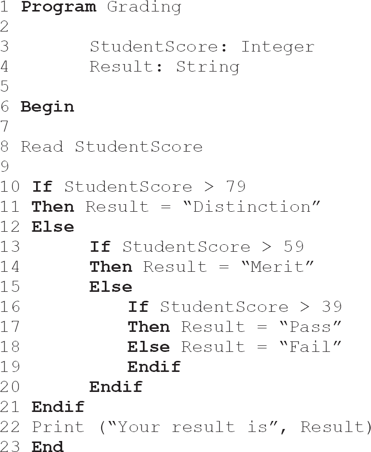
How many test cases are needed for 100 per cent statement coverage?
The answer can be found at the end of the chapter.
Exercise 4.8
Now using the program Grading in Exercise 4.7 again, try to calculate whether 100 per cent statement coverage is achieved with a given set of data.
Suppose we ran two test cases, as follows:
Test Case 1 StudentScore = 50
1. Would 100 per cent statement coverage be achieved?
2. If not, which lines of pseudo code will not be exercised?
The answer can be found at the end of the chapter.
Decision testing and coverage
Decision testing aims to ensure that the decisions in a program are adequately exercised. Decisions, as you know, are part of selection and iteration structures; we see them in IF THEN ELSE constructs and in DO WHILE or REPEAT UNTIL loops. To test a decision, we need to exercise it when the associated condition is true and when the condition is false; this guarantees that both exits from the decision are exercised.
As with statement testing, decision testing has an associated coverage measure and we normally aim to achieve 100 per cent decision coverage. Decision coverage is measured by counting the number of decision outcomes exercised (each exit from a decision is known as a decision outcome) divided by the total number of decision outcomes in a given program. It is usually expressed as a percentage.
The usual starting point is a control flow graph, from which we can visualise all the possible decisions and their exit paths. Have a look at the following example.

This program has a WHILE loop in it. There is a golden rule about WHILE loops. If the condition at the WHILE statement is true when the program reaches it for the first time, then any test case will exercise that decision in both directions because it will eventually be false when the loop terminates. For example, as long as Index is less than Count when the program reaches the loop for the first time, the condition will be true and the loop will be entered. Each time the program runs through the loop it will increase the value of Index by one, so eventually Index will reach the value of Count and pass it, at which stage the condition is false and the loop will not be entered. So, the decision at the start of the loop is exercised through both its true exit and its false exit by a single test case. This makes the assumption that the logic of the loop is sound, but we are assuming that we are receiving this program from the developers, who will have debugged it.
Now all we have to do is to make sure that we exercise the If statement inside the loop through both its true and false exits. We can do this by ensuring that the input stream has both negative and positive numbers in it.
For example, a test case that sets the variable Count to 5 and then inputs the values 1, 5, −2, −3, 6 will exercise all the decisions fully and provide us with 100 per cent decision coverage. Note that this is considered to be a single test case, even though there is more than one value for the variable New, because the values are all input in a single execution of the program. This example does not provide the smallest set of inputs that would achieve 100 per cent decision coverage, but it does provide a valid example.
Although programs with loops are a little more complicated to understand than programs without loops, they can be easier to test once you get the hang of them.
DECISION TESTING – EXAMPLE 4.7
Let us try an example without a loop now.
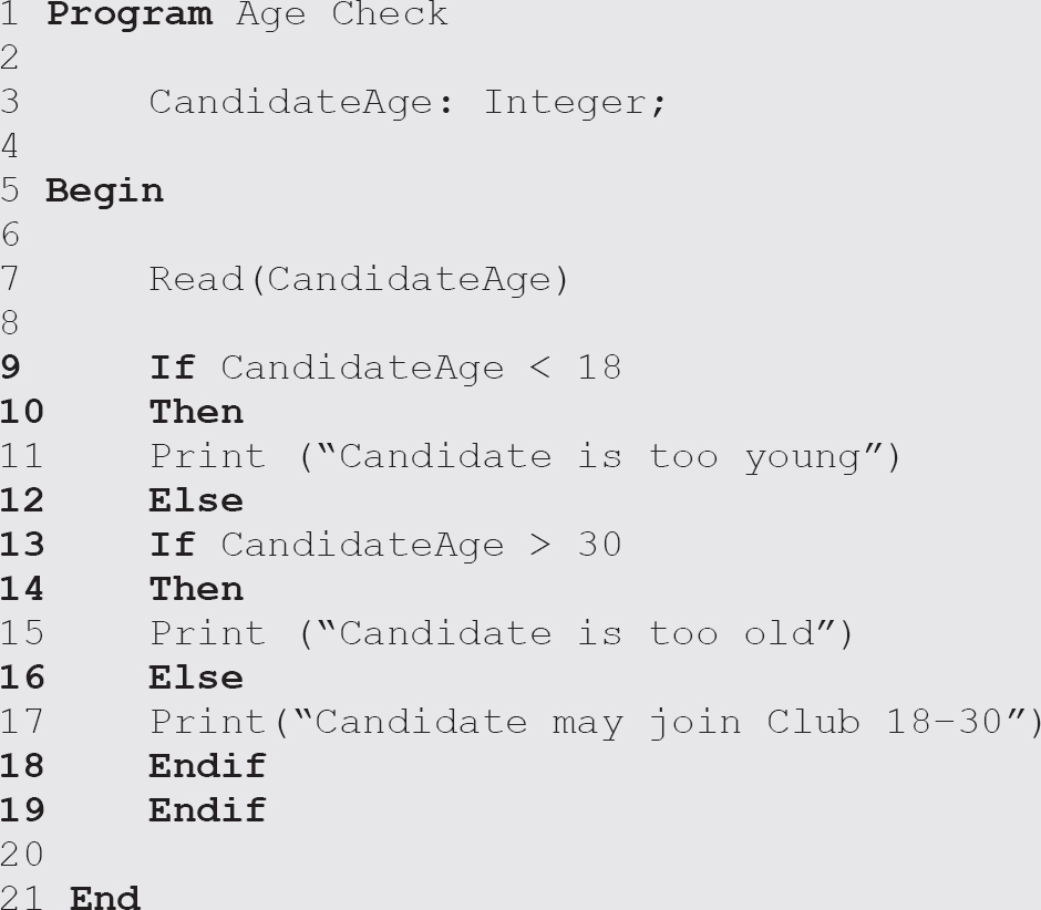
Have a go at calculating how many test cases are needed for 100 per cent decision coverage and see if you can identify suitable test cases.
Figure 4.14 shows the flow graph drawn in the hybrid flow graph format.
Figure 4.14 Paths through the hybrid flow graph – Example 4.7
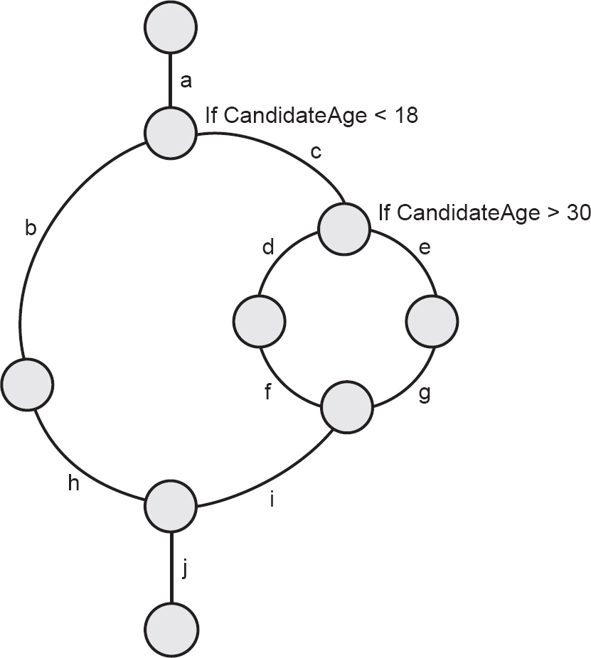
How many test cases will we need to achieve 100 per cent decision coverage? Well each test case will just run through from top to bottom, so we can only exercise one branch of the structure at a time.
We have labelled the path fragments a, b, c, d, e, f, g, h, i, j and you can see that we have three alternative routes through the program – path abhj, path acegij and path acdfij. That needs three test cases.
The first test case needs decision 1 to be true – so CandidateAge = 16 will be OK here. The second needs to make the first decision false and the second decision true, so CandidateAge must be more than 18 and more than 30 – let us say 40. The third test case needs the first decision to be false and the second decision to be false, so CandidateAge of 21 would do here. (You cannot tell which exit is true and which is false in the second decision; if you want to, you can label the exits T and F, though in this case it does not really matter because we intend to exercise them both anyway.)
So, we need three test cases for 100 per cent decision coverage:
CandidateAge = 16
CandidateAge = 21
CandidateAge = 40
which will exercise all the decisions.
Note that when we are testing decisions, we need to exercise the true and false outcomes of each decision, even if one of these has no statements associated with it. So, decision coverage gives us that little bit extra in return for a little more work. One hundred per cent decision coverage guarantees 100 per cent statement coverage, but 100 per cent statement coverage may be less than 100 per cent decision coverage.
CHECK OF UNDERSTANDING
1. What is the purpose of decision testing?
2. How many test cases are needed to exercise a single decision?
3. How many test cases are needed to exercise a loop structure?
Exercise 4.9
This program reads a list of non-negative numbers terminated by −1.
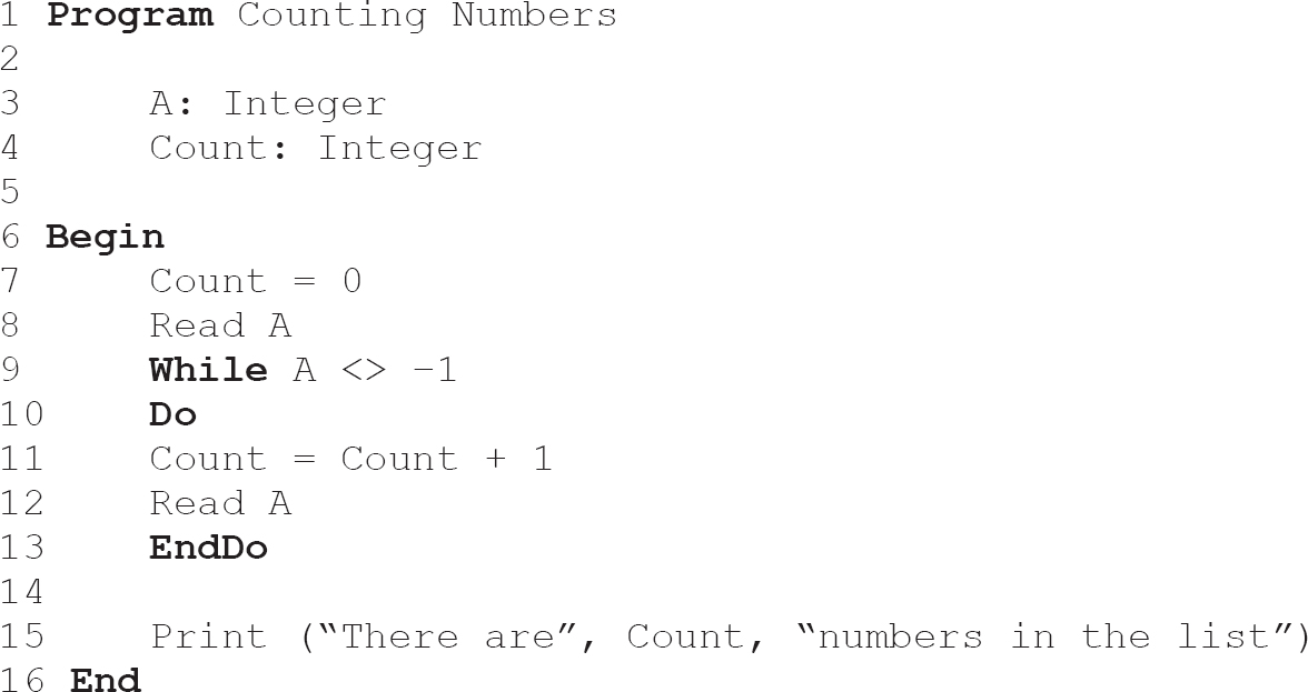
How many test cases are needed to achieve 100 per cent decision coverage?
The answer can be found at the end of the chapter.
Exercise 4.10
Using Program Counting Numbers from Exercise 4.9, what level of decision coverage is achieved by the single input A = –1?
The answer can be found at the end of the chapter.
Simplified control flow graphs
Simplified control flow graphs (CFGs) share the format used for flow charts. They incorporate less detail, since their purpose is to identify control structures but not the detail of code. The testing literature sometimes provides examples and questions using simplified CFGs instead of code, so this section deals with the interpretation of simplified CFGs and provides examples and exercises that cover these structures.
In simplified CFGs, a sequence of code is presented as one or more boxes in a line. Strictly speaking, only a single box is needed but additional boxes are sometimes included to make the CFG easier to follow. Decisions are represented by a single box with two exits, usually labelled T and F (for True and False respectively).
Figure 4.15 shows a simplified CFG depicting a sequence of code followed by a decision based on the evaluation of a decision.
Figure 4.15 Simplified control flow graph: a decision
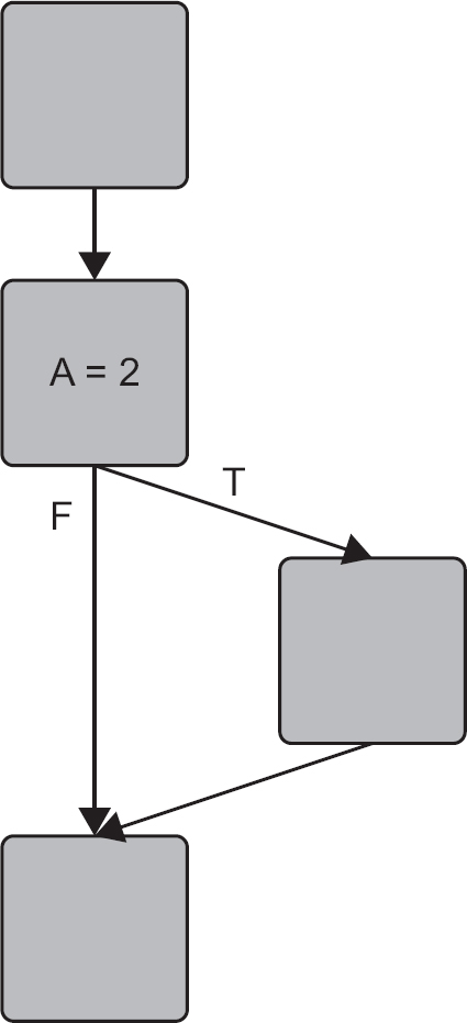
Looping structures can have a decision at the beginning of the loop or at the end (see Figure 4.16).
Figure 4.16 Simplified control flow graph: location of a decision in a loop
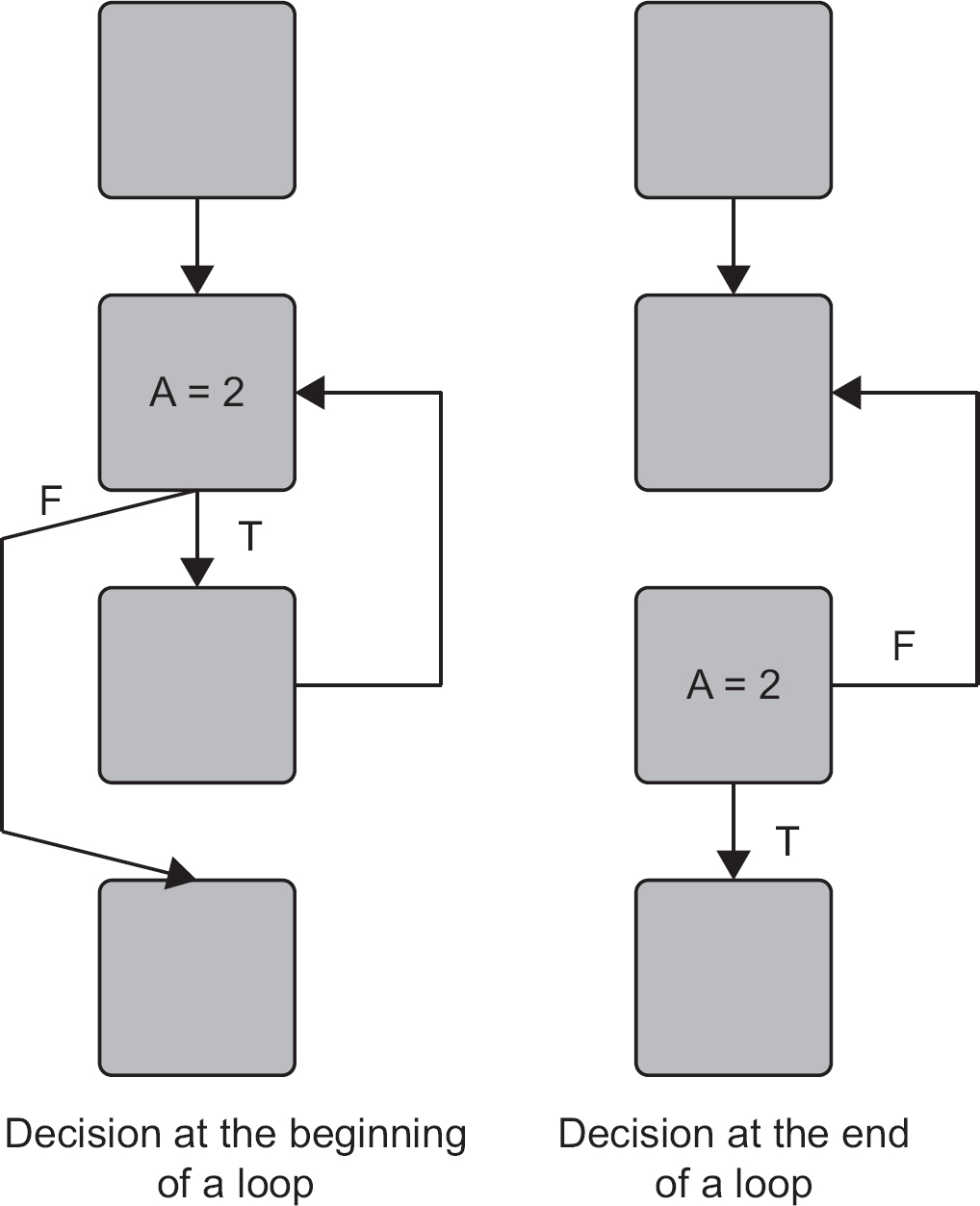
Here is an example of how simplified CFGs are read and interpreted for simple structures.
SIMPLIFIED CONTROL FLOW GRAPHS – EXAMPLE 4.8
Figure 4.17 Example of how simplified control flow graphs are read and interpreted
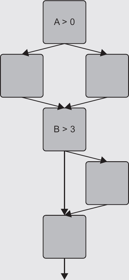
Which of the following pairs of tests achieve 100 per cent decision coverage for the structure shown in Figure 4.17?
a. A = 1, B = 2; A = 0, B = 1
b. A = 2, B = 4; A = 1, B = 2
c. A = 3, B = 0; A = 0, B = 1
d. A = 0, B = 4; A = 1, B = 3
Answer – The correct answer is d.
Option a. In the first decision A is greater than zero in the first test and equals zero in the second, so this decision has been exercised in both directions. B is less than 3 in both tests, so decision B > 3 is not exercised in both directions. Therefore 100 per cent decision coverage has not been achieved.
Option b. A is greater than zero in both tests, so the decision A > 0 has not been exercised in both directions. Therefore 100 per cent decision coverage has not been achieved.
Option c. A is greater than zero in test 1 and equals zero in test 2, so decision A > 0 has been exercised in both directions. B is less than 3 in both tests, so decision B > 3 has not been exercised in both directions. Therefore 100 % decision coverage has not been achieved.
Option d. A equals zero on test 1 and equals 1 in test 2, so test A > 0 has been exercised in both directions. B is greater than 3 in test 1, but not in test 2, so decision B > 3 has been exercised in both directions. Therefore 100 per cent decision coverage has been achieved.
SIMPLIFIED CONTROL FLOW GRAPHS – 50 PER CENT DECISION COVERAGE – EXAMPLE 4.9
Using the same diagram as in Example 4.8, which of the following sets of test cases achieve 50 per cent decision coverage?
a. A = 1, B = 2; A = 0, B = 3
b. A = 0, B = 4; A = 1, B = 3
c. A = 1, B = 2; A = 2, B = 2
d. A = 5, B = 4; A = 0, B = 3
Answer – The correct answer is c.
Option a. The decision A > 0 has been exercised in both directions, but decision B > 3 has been exercised in only one direction. Therefore, the decision coverage would be 3/4 or 75 per cent.
Option b. The decision A > 0 has been exercised in both directions and decision B > 3 has been exercised in both directions. Therefore, the decision coverage would be 4/4 or 100 per cent.
Option c. The decision A > 0 has not been exercised in both directions and decision B > 3 has not been exercised in both directions. Therefore, the decision coverage is 2/4 or 50 per cent.
Option d. The decision A > 0 has been exercised in both directions and decision B > 3 has been exercised in both directions. Therefore, the decision coverage would be 4/4 or 100 per cent.
Exercise 4.11
In the simplified CFG shown in Figure 4.18, which of the following sets of test cases achieve 100 per cent statement coverage?
Figure 4.18 Control flow graph for Exercise 4.11
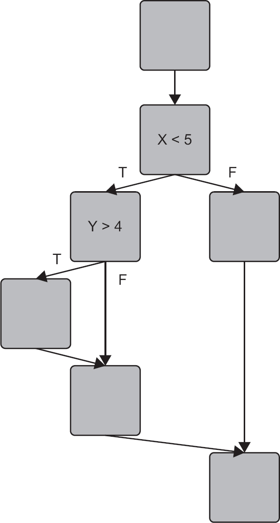
a. X = 7, Y = 6; X = 3, Y = 5
b. X = 3, Y = 3; X = 4, Y = 4
c. X = 6, Y = 5; X = 1, Y = 1
d. X = 5, Y = 4; X = 4, Y = 4
The answer can be found at the end of the chapter.
Exercise 4.12
In the same CFG shown in the previous exercise, how many test cases are required to achieve 100 per cent decision coverage?
a. 1
b. 2
c. 3
d. 4
The answer can be found at the end of the chapter.
There are further questions for you to try at the end of this chapter.
Other white-box test techniques
More sophisticated techniques are available to provide increasingly complete code coverage. In some applications these are essential: for example, in a safety-critical system it is vital to know that nothing unacceptable happens at any point when the code is executed. Would you like to ‘fly by wire’ if you did not know what was happening in the software? The many well-documented mishaps in computer-controlled systems provide compelling examples of what can happen if code – even code that is not providing essential functionality in some cases – does something unexpected. Measures such as condition coverage and multiple condition coverage are used to reduce the likelihood that code will behave in unpredictable ways by examining more of it in more complex scenarios.
Coverage is also applicable to other types and levels of structure. For example, at the integration level it is useful to know what percentage of modules or interfaces has been exercised by a test suite, while at the functional level it is helpful to step through all the possible paths of a menu structure. We can also apply the idea of coverage to areas outside the computer; for example, by exercising all the possible paths through a business process as testing scenarios.
Exercise 4.13
Figure 4.19 Test case for Exercise 4.13
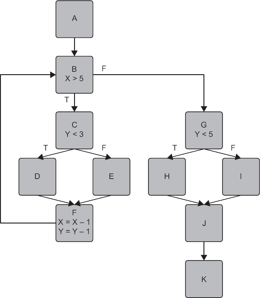
Using Figure 4.19, test case 1 is executed with the values X = 6, Y = 2. Which of the following paths will be executed by test case 1?
a. ABCEFBGIJK
b. ABCDFBGIJK
c. ABCDFBGHJK
d. ABCDFBCEFGHJK
Exercise 4.14
In Figure 4.20, the goal for the project is 100 per cent decision coverage and the following tests have so far been executed:
• Test 1 covers path ABCDFBGHJK.
• Test 2 covers path ABGIJK.
Figure 4.20 Test case for Exercise 4.14

Which of the following statements about decision coverage is correct?
a. Decision B has not been tested completely.
b. 100 per cent decision coverage has been achieved.
c. Decision G has not been tested completely.
d. Decision C has not been tested completely.
The main examinable material continues from here.
EXPERIENCE-BASED TECHNIQUES
Experience-based techniques are those that you fall back on when there is no adequate specification from which to derive specification-based test cases or no time to run the full structured set of tests. They use the users’ and the testers’ experience to determine the most important areas of a system and to exercise these areas in ways that are both consistent with expected use (and abuse) and likely to be the sites of errors – this is where the experience comes in. Even when specifications are available, it is worth supplementing the structured tests with some that you know by experience have found defects in other similar systems.
Techniques range from the simplistic approach of ad hoc testing or error guessing through to the more sophisticated techniques such as exploratory testing, but all tap the knowledge and experience of the tester rather than systematically exploring a system against a written specification.
Error guessing
Error guessing is a very simple technique that takes advantage of a tester’s skill, intuition and experience with similar applications to identify special tests that may not be easy to capture by the more formal techniques. When applied after systematic techniques, error guessing can add value in identifying and exercising test cases that target known or suspected weaknesses or that simply address aspects of the application that have been found to be problematical in the past.
The main drawback of error guessing is its varying effectiveness, depending as it does on the experience of the tester deploying it. However, if several testers and/or users contribute to constructing a list of possible errors and tests are designed to attack each error listed, this weakness can be effectively overcome. Another way to make error guessing more structured is by the creation of defect and failure lists. These lists can use available defect and failure data (where this exists) as a starting point, but the list can be expanded by using the testers’ and users’ experience of why the application under test in particular is likely to fail. The defect and failure list can be used as the basis of a set of tests that are applied after the systematic techniques have been used. This systematic approach is known as fault attack.
Exploratory testing
Exploratory testing is a technique that combines the experience of testers with a structured approach to testing where specifications are either missing or inadequate and where there is severe time pressure. It exploits concurrent test design, test execution, test logging and learning within time-boxes and is structured around a test charter containing test objectives. In this way exploratory testing maximises the amount of testing that can be achieved within a limited time frame, using test objectives to maintain focus on the most important areas.
Checklist-based testing
Checklist-based testing is testing based on high-level checklists, which may be drawn from many sources and generally encapsulate individuals’ experience and information gleaned from other sources, such as standards, known problem areas, expected use scenarios and any other relevant sources. Checklists are a guide to the testing required, so are used mainly by experienced testers as a source of ideas from which detailed tests are derived.
The checklist is drawn up during test analysis as a set of test conditions and may reuse or update previous checklists. Checklists can support both functional and non-functional testing. Coverage is defined by completion of the checklist and may be higher than for other forms of testing, though repeatability will typically be lower than for more formal testing.
SYSTEMATIC AND EXPERIENCE-BASED TECHNIQUES
How do we decide which is the best technique? There are some simple rules of thumb:
1. Always make functional testing the first priority. It may be necessary to test early code products using structural techniques, but we only really learn about the quality of software when we can see what it does.
2. When basic functional testing is complete that is a good time to think about test coverage. Have you exercised all the functions, all the requirements, all the code? Coverage measures defined at the beginning as exit criteria can now come into play. Where coverage is inadequate, extra tests will be needed.
3. Use structural methods to supplement functional methods where possible. Even if functional coverage is adequate, it will usually be worth checking statement and decision coverage to ensure that enough of the code has been exercised during testing.
4. Once systematic testing is complete, there is an opportunity to use experience-based techniques to ensure that all the most important and most error-prone areas of the software have been exercised. In some circumstances, such as poor specifications or time pressure, experience-based testing may be the only viable option.
1. What is meant by experience-based testing?
2. Briefly compare error guessing and exploratory testing.
3. When is the best time to use experience-based testing?
SUMMARY
In this chapter we have considered the most important terminology needed in discussing the specification stage of a generalised test process, which was introduced in Chapter 1. We explained how test conditions are derived and how test cases can be designed and grouped into test procedures for execution.
Test design techniques were categorised into three main groups known as specification-based or black-box techniques, structure-based or white-box techniques, and experience-based techniques.
The specification-based techniques introduced were equivalence partitioning, boundary value analysis, state transition testing, decision table testing and use case testing. Specific worked examples of all except use case testing were given (and this was excluded solely because the examination does not require the ability to generate test cases from use cases). Structure-based techniques were introduced and worked examples were given for statement testing and decision testing. Experience-based techniques introduced included error guessing and exploratory testing.
Finally, the factors involved in selecting test case design techniques were discussed and guidance given on the selection criteria to be applied.
Example examination questions with answers
E1. K2 question
Which of the following correctly characterises white-box test techniques?
a. Test cases may be used to detect differences between requirements and implementation.
b. Test cases may be used to determine deviations from requirements.
c. Test cases may be based on software architecture and used to exercise interfaces.
d. Test cases may be based on user stories and used to exercise use cases.
E2. K2 question
Which of the following identifies a key difference between black-box and white-box test techniques?
a. Coverage measures are applied to white-box test cases but not to black-box test cases.
b. Black-box test cases may be based on requirements or on the tester’s experience; white-box test cases are based on structure.
c. Coverage measures are applied to black-box test cases but not to white-box test cases.
d. Black-box tests can determine deviations from requirements; white-box test can determine deviations from design.
E3. K3 question
A washing machine has three temperature bands for different kinds of fabrics: fragile fabrics are washed at temperatures between 15 and 30 degrees Celsius; normal fabrics are washed at temperatures between 31 and 60 degrees Celsius; heavily soiled and tough fabrics are washed at temperatures between 61 and 100 degrees Celsius.
Which of the following contains only values that are in different equivalence partitions?
a. 15, 30, 60
b. 20, 35, 60
c. 25, 45, 75
d. 12, 35, 55
Which of the following correctly identifies the derivation of test cases in use case testing?
a. Test cases are derived solely from interactions between human actors and system subjects.
b. Test cases can be based on interactions and activities represented by workflows, which must be represented graphically.
c. Test cases can be derived from defined behaviours, alternative or exceptional behaviours, or error handling behaviours.
d. Test cases specify behaviour that a single subject can perform in collaboration with a single actor.
E5. K3 question
Which one of the following statements is correct?


a. The given test cases cover both valid and invalid transitions in the state transition diagram.
b. The given test cases represent only the possible valid transitions in the state transition diagram.
c. The given test cases represent only some of the valid transitions in the state transition diagram.
d. The given test cases represent sequential pairs of transitions in the state transition diagram.
Answers to questions in the chapter
SA1. The correct answer is d.
SA2. The correct answer is d.
SA3. The correct answer is b.
Exercise 4.1
The partitions are: £0.00–£1,000.00, £1,000.01–£2,000.00, and >= £2,000.01.
Exercise 4.2
The valid partitions are: £0.00–£20.00, £20.01–£40.00, and >= £40.01. Non-valid partitions would include negative values and alphabetic characters.
Exercise 4.3
The partitions are: question scores 0–20; total 0–100; question differences: 0–3 and > 3; total differences 0–10 and > 10.
Boundary values are: −1, 0, 1 and 19, 20, 21 for the question scores; −1, 0, 1 (again) and 99, 100, 101 for the question paper totals; −1, 0, 1 (again) and 2, 3, 4 for differences between question scores for different markers; and −1, 0, 1 (again) and 9, 10, 11 for total differences between different markers.
In this case, although the −1, 0, 1 values occur several times, they may be applied to different parts of the program (e.g. the question score checks will probably be in a different part of the program from the total score checks) so we may need to repeat these values in the boundary tests.
Exercise 4.4
Billy will be eligible for a cash payment but not for a share allocation.
Exercise 4.5
The correct answer is b.
Option a includes the transition DE; option c includes the transition CE; option d includes the transition FA. None of these is valid from the diagram.
Exercise 4.6
The flow chart is shown in Figure 4.21. The control flow graph is shown in Figure 4.22.
Exercise 4.7
The answer is four because there are three decisions and every outcome has an executable statement in it.
Figure 4.21 Flow chart for Exercise 4.6
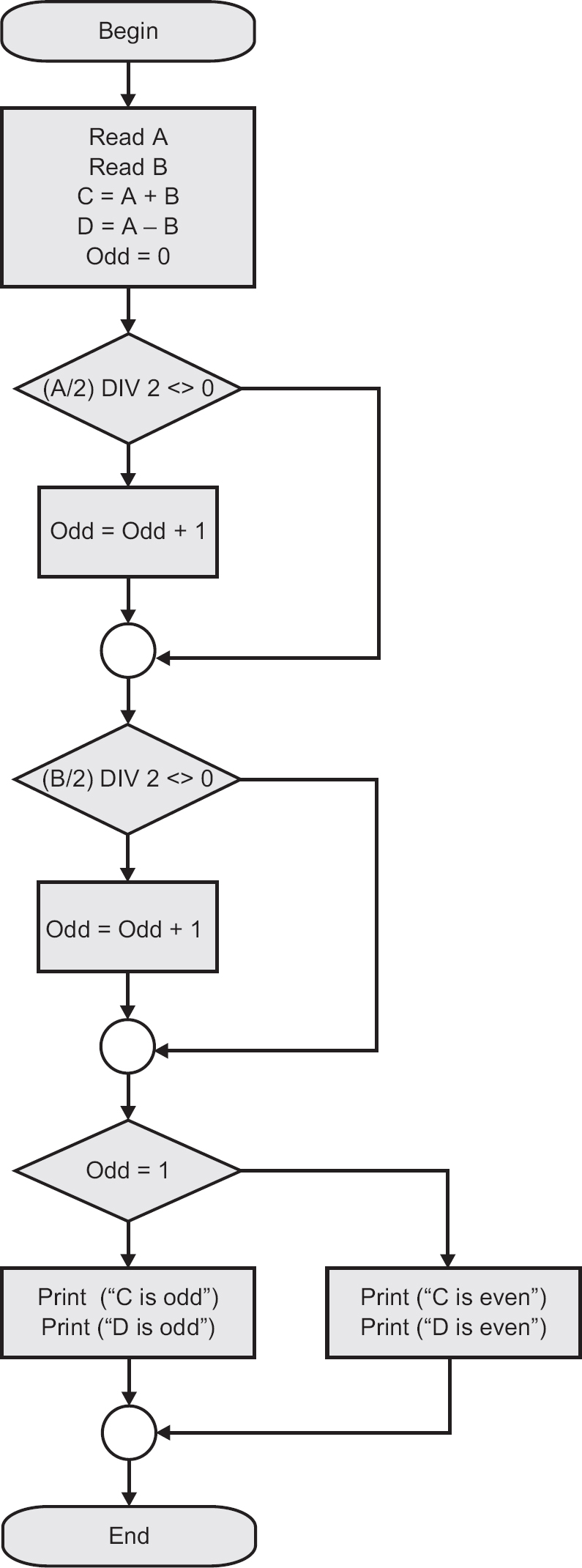
Figure 4.22 Control flow graph for Exercise 4.6
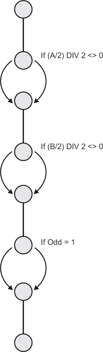
Exercise 4.8
1. No, 100 per cent statement coverage would not be achieved. We know from Exercise 4.7 that four test cases are needed.
2. Statements 11 and 14 would not be exercised because they need inputs higher than 79 and 59 respectively.
Exercise 4.9
The answer is one because a single list terminated by −1 (say 4, 6, 3, −1) will enter the loop the first three times and then exit on the fourth; hence the WHILE decision will be true three times and then false, which exercises the decision in both directions with one test case.
A single test case with values of 1, −1 would also exercise all decisions.
Exercise 4.10
Decision coverage of 50 per cent will be achieved. The –1 input will make the While condition False and the loop will not be entered. The program will print the message ‘There are 0 integers in the list’ and terminate, so the True outcome of the decision will not be exercised.
Exercise 4.11
The correct answer is a.
There are statements in the false exit from decision X < 5 and in the true exit from decision Y > 4, so we need two tests because the test that makes X < 5 false will bypass the decision Y > 4. One of the test cases can be any pair of values that has X >= 5, so X can be 5 or more and Y is irrelevant. In the other test, X must be less than 5 and Y must also be greater than 4. Many pairs of values, such as X = 4, Y = 5, would be suitable. The two tests must have X >= 5 in one test and X < 5 AND Y > 4 in the other. Option a meets these criteria. Option b has X < 5 in both tests, so it cannot be correct. Option c has one test with X > 5 but, although the other test has X < 5, it also sets Y to 1, so Y > 4 is not true. Option d has X = 5 in one test and X < 5 in the other, but in this case the value of Y is 4, so Y > 4 is not true.
Exercise 4.12
The correct answer is c.
In this case we must not only execute every branch with a statement in it, but we must exercise every decision in both its true and false states. We could arrive at the correct answer by recognising that the CFG has two regions and two decisions. The questions regions + 1 and decisions + 1 both give the answer 3. We could also work it out from first principles. The paths we would need to follow would be:
1. False through X < 5
2. True through X < 5 AND True through Y > 4
3. True through X < 5 AND False through Y > 4
These three tests would exercise both decisions in their true and false states and would therefore achieve 100 per cent decision coverage.
Exercise 4.13
The correct answer is c.
For a to be true, Y >= 3 would have to be true. For b to be true, Y >= 5 would have to be true. For d to be true, Y >= 3 would have to be true after one traversal of the loop.
Exercise 4.14
The correct answer is d.
Option a is not true because B was exercised one way in test case 1 and the other way in test case 2. Option b is not true because E has not been traversed, which means that decision E has not been exercised in both directions. Option c is not true because decision G is exercised one way in test case 1 and the other way in test case 2.
Answers to example examination questions
E1. The correct answer is c.
White-box techniques are about the structure of software solutions, so they typically exercise interfaces and check that the software architecture has been correctly implemented. They do not reference requirements as such, and therefore cannot determine deviations from requirements or whether requirements have been correctly implemented. User stories are a form of requirements, so white-box testing is not appropriate to user stories or use cases.
E2. The correct answer is d.
Answer a is incorrect because coverage measures can be applied to both black-box and white-box tests. Answer b is partially correct, in that white-box test cases are based on structure, and black-box test cases are based on requirements but not the tester’s experience. Experience-based testing is based on the tester’s experience. Option c is incorrect for the same reason as option a is incorrect. Option d is the correct answer because black-box testing is based on requirements and white-box testing is based on design.
E3. The correct answer is c.
Option a includes two values from the lower partition; option b contains two values from the second partition; option d contains one value that is invalid (out of range).
E4. The correct answer is c.
Option a is incorrect because test cases are not solely based on interactions and may also incorporate preconditions and postconditions. Option b is incorrect because workflows are not the only option for describing interactions; activity diagrams or business process models are other alternatives. Option d is incorrect because a use case may represent interactions between a subject and one or more actors. Option c is correct; use cases may represent defined behaviours, alternative or exceptional behaviours, and error handling behaviours.
E5. The correct answer is a.
Option a is correct because the test cases represent all the valid transitions and one possible invalid transition. Option b is incorrect because the test cases recognise one invalid transition. Option c is incorrect because the test cases represent all of the valid transitions. Option d is incorrect because none of the test cases represents sequential pairs of transitions.