CHAPTER 4

Covered with Oil

Incorporating Realism in Cost and Schedule Risk Analysis

Jimmy Buffett’s most popular song is “Margaritaville.” The easy-listening rock hit has spawned a variety of merchandise, including a restaurant chain. The 1977 song is set in a tropical climate. One of the lines in the song’s lyrics refers to beachgoers covered in tanning oil. Jimmy Buffett probably never imagined that this could apply to crude oil instead. However, the 2010 oil spill in the Gulf of Mexico resulted in oily beaches on the US Gulf Coast. Both the cost and environmental impacts were much worse than anyone had predicted. It was the biggest oil spill ever. The leak wasted more than five million barrels of oil and was an environmental disaster.¹ This natural disaster is an example of a black swan event. Not planning for some events such as this one outside of a project’s control is reasonable. But project managers have some control over their destiny. They can meet budget, schedule, and scope by cutting content. In the cases of extreme overruns, senior leaders can cancel projects. However, budgets for projects typically include little risk reserves. Most risk analyses do not account for minimal changes in a project’s design or relatively mild external forces that should be part of the initial plan.

TYPES OF RISK

Previous chapters discussed two broad categories of cost and schedule growth—internal and external. These are also sources of risk. Another factor is estimating uncertainty, which accounts for two different phenomena. One is that not all program characteristics are known with certainty when estimating. These change significantly from the start of a program to its completion. The other is that even for past data, no model can accurately predict cost or schedule with 100% accuracy. This is true even if program characteristics do not change. Risk analyses typically cover some of these risks. Those typically excluded are black swan events such as the Gulf Oil spill, and good reasons exist to leave out the most extreme events. Risk analysis is intended to provide decision makers with information to help them successfully manage projects. Inclusion of some extreme events with large impacts will not aid decision makers in managing their projects. Thus, exclusion of some risks is advisable. However, over the course of a major development, it is likely that some of these external factors may impact costs across an organization.

Donald Rumsfeld, Secretary of Defense under Presidents Gerald Ford and George W. Bush once stated, “As we know, there are known knowns; there are things we know. We know also there are known unknowns; that is to say, we know there are some things we do not know. But there are also unknown unknowns—the ones we don’t know we don’t know.”² The “unknown unknowns” have the biggest impact on projects. They may not be likely to occur, but they have outsized consequences. For a test event, a known known could be a three-day schedule slip. These happen regularly for large test events and are usually incorporated in project plans. A known unknown is a test failure. They are known to happen, but no one knows when they will occur. Cost and schedule reserves are typically not set aside for these events. Numerous project managers have told me that they do not plan for failure, which is a common excuse to avoid planning for or acknowledging risk.³ I worked on one program that had a test failure that led to a complete re-test. This doubled the total cost of the test event. The impact was an extra $100 million and a one-year delay in the schedule for completing development tests. The unwillingness to plan for risks is also common in infrastructure projects and has even been given a title—the “Everything Goes According to Plan” principle.⁴ An unknown unknown could be a hurricane in the Pacific that wipes out the test range infrastructure. This would cause significant cost impacts and long delays in test schedules.

While it is good to exclude some risks, cost and schedule estimates tend to exclude factors that should be incorporated in risk analysis. This includes most estimating uncertainty. For example, the greater uncertainty inherent when estimates are based on small data sets is not considered. The extent to which requirements will change is underestimated. The uncertainty inherent in the degree of heritage from previous, similar programs that can be relied upon is not considered. The amount of technology development that will need to be conducted is taken too lightly. As a result, early project plans sometimes have more in common with science fiction than science fact. For example, one satellite project several years ago maintained that it was developing an apogee kick motor for a project that would be a near carbon copy of a previous one, but the new motor would be twice the size as the close analogy. When looking at the final cost, it was easy to see that a relatively large amount of design cost was required. As mentioned in the discussion on cost and schedule growth, this inherent optimism seems to be common. This optimism reduces the estimate of cost and schedule. Also, it lowers the perceived amount of risk.

Project managers are not the only ones who do not understand risk. As a society, we are risk blind. “There is a blind spot: when we think of tomorrow we do not frame it in terms of what we thought about yesterday on the day before yesterday. Because of this introspective defect we fail to learn about the difference between our past predictions and the subsequent outcomes. When we think of tomorrow, we just project it as another yesterday.”⁵ Just as the cow who jumped over the moon didn’t think about the risks of re-entering the atmosphere, so individuals tend to underestimate risk ranges.

I mentioned Hofstadter’s Law in Chapter 1, which was “it always takes longer than you think, even taking into account Hofstadter’s Law.” As time is money, my cost corollary to Hofstadter’s Law is: It always costs more than you think, even taking into account it will cost more than you think. A second, similar corollary regarding risk is: It is always riskier than you think, even taking into account that it is riskier than you think.

THE TRACK RECORD FOR RISK ANALYSIS

One of the ways to get better at something is to measure performance. By doing so, you can assess what you did right and what you did wrong. You can figure out your mistakes and learn from them. You can also see what you did right and learn to do that again. This feedback is critical for improving performance. Projects would have better risk analyses if the profession as a whole had been doing this on a systematic basis for the past 50 years. However, this is rarely done. These actions over the years are like throwing darts but never looking at the dartboard to see how close the darts are to the bull’s-eye. Without looking at the results, it is impossible to determine if the methods used hit the bull’s-eye or missed the dartboard entirely.

There is a small amount of data on performance of cost risk analysis and even less for schedule risk analysis. Not surprisingly, what is available indicates that risk analyses are far from realistic. For most analyses I have examined, the actual cost is above the 90% confidence level. If done right, a 90% confidence level should be exceeded by only one out of 10 projects. However, I have found the opposite to be true. A severe disconnect exists between risk analysis of cost and schedule and the actual cost and schedule. The statistician George Box famously remarked that “all models are wrong, but some are useful.” He went on to further state “the approximate nature of the model must always be borne in mind.”⁶ As discussed in the previous chapter, single-best estimates are sure to be wrong. That is why risk analysis is needed—to cover the range of variation. The problem is that this variation is consistently underestimated. See Table 4.1 for data on 10 projects for which a quantitative cost risk analysis was conducted.

Table 4.1 Cost Growth and Ratio of Actual Cost to 90% Confidence Level for 10 Historical Projects

The projects in Table 4.1 are from a variety of applications.⁷ I conducted cost and schedule risk analyses for two of the projects in the table, including the one at the top of the table. It was a relatively rare mission that did not experience cost growth. My estimate of the 50% confidence level was within 1% of the actual cost. The project also completed on time, in line with my 50% confidence level for schedule. This kind of outcome is the exception rather than the rule. As can be seen from the table, all the other missions experienced significant cost growth. Even so, 90% confidence levels should have been high enough to capture these variations. However, the actual cost was greater than the 90% confidence level for 8 of the 10. This dismal result is even worse than it appears. Two of the missions listed in the table were cancelled. If they had not been cancelled, the cost growth would have been higher. The fifth project in the table experienced such significant growth from one phase to the next that it exceeded the 90% confidence level well before completion. For 5 of the 10 missions, the actual cost was at least one and a half times the 90% confidence level, and for 2 it was double or more. The term “90% confidence level” for these analyses is grossly erroneous. If it were accurate, for 10 projects, the chance that 2 or fewer would be less than or equal to the 90% confidence level is one in 2.7 million.⁸ For the tenth project, the one with the highest cost growth among those listed in the table, a schedule risk analysis was even worse than the cost risk analysis in capturing the actual variation. The actual schedule was 2.8 times greater than the 90% confidence level for the schedule analysis. The ugly truth is that for most projects, the actual cost and schedule will not even be on the S-curve.

Risk is underestimated for several reasons. One is the influence of optimism that we discussed earlier. Just as optimism causes the baseline cost to be too low and the schedule to be too short, it also causes risk ranges to be too tight. The use of distributions that do not have enough variation, such as the triangular and Gaussian distributions we discussed in the last chapter, is a second factor in underestimating risk. A third important cause is neglecting to incorporate correlation.

THE IMPORTANCE OF CORRELATION

The number of shark attacks and ice cream sales at a beach tend to move in tandem with one another. As shark attacks rise, so do ice cream sales. When shark attacks decrease, ice cream sales wane as well. This tendency is called correlation. That does not mean that one causes the other. An increase in ice cream sales does not cause shark attacks. Conversely, an increase in shark attacks does not cause ice cream sales to rise. Correlation is not the same as causation. The two tend to move together because they are driven by a common cause, which is the weather. As temperatures rise in the spring and summer, more people visit beaches. More people at a beach means there are more customers for ice cream and more potential shark attack victims too.

Correlation is a number between –1.0 and +1.0. When two events tend to move in the same direction—when one increases the other increases and when one decreases the other decreases—correlation is positive. When two events tend to move in opposite directions, correlation is negative. Positive correlation is much more common than negative correlation because of the common entropic forces acting on a project during its life cycle. Many of these have a common source, such as an economic downturn that stresses budgets for a multitude of projects, which in turn results in schedule slips as projects have less money in the near term.

Despite its importance, correlation is often ignored in both cost and schedule risk analysis. This is a major cause of underestimation of risk. Recall that probability distributions have a central tendency and a spread around this central tendency. The variation around the central tendency is typically measured with the standard deviation. As the standard deviation of total cost is a function of the standard deviations of the individual elements in the Work Breakdown Structure and the correlation between them, it is impossible to avoid making a choice about correlation. If you ignore it, you are assuming no correlation. Thus, an estimator who disregards correlation is making a choice about correlation—the wrong choice, since assuming no correlation will lead to underestimation of total aggregate risk.

If the elements have a functional relationship between them in a cost estimate, a functional correlation will automatically be incorporated in a simulation. For example, if the cost of project management is estimated as 10% of the total direct cost, the two are functionally correlated. A simulation will account for this. As total direct cost varies, so will project management cost. However, in most estimates at least some of the elements will not capture this. For these elements, correlation must be assigned. The number of correlations grows rapidly as a function of the number of elements. The correlation between an element and itself is 1.0. Correlation is also symmetric, so, for example, in a 100-element Work Breakdown Structure with no functional correlation present, there are 0.5 × (100² –100) = 4,950 correlations to assign. Because of the large number of correlations, a single value is typically used in practice. However, there is no single best value to use.

See Figure 4.1 for a graph that shows how much the total standard deviation will be underestimated when correlation is assumed to be zero between all elements. This graph is for 30 Work Breakdown Structure elements. For example, if the actual correlation is 20%, but it is assumed to be zero between all elements, then the total standard deviation will be underestimated by 60%. The amount of underestimation increases with the size of the Work Breakdown Structure.

Figure 4.1 Impact of Correlation on Cost Risk

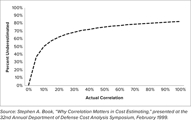
Notice in Figure 4.1 that there is an apparent knee in the curve around 20%. Above 20% correlation, the consequence of assuming zero correlation begins to dwindle. This graph is the basis for assuming 20% to 30% for a rule of thumb.⁹ However, the graph in Figure 4.2 does not tell us how much the risk is underestimated because correlation is assumed to be 20% but is really 60%. Thus, the widespread use of 20% correlation may not be enough. For example, for a 100-element WBS, if the correlation is assumed to be 20% but instead is 60%, it turns out that the total standard deviation is significantly underestimated. The knee-in-the-curve approach still leads to significant underestimation of correlation. A more robust approach to assigning correlations would be to use the value that results in the least amount of error when you are wrong, which is likely to be the case. This approach is robust in the sense that without solid evidence to assign a correlation value, it minimizes the amount by which the total standard deviation is underestimated or overestimated due to the correlation assumption. Using this method, I have derived a recommended value in the absence of other information of 60%, much higher than the 20% knee in the curve.¹⁰ See Figure 4.2.

Figure 4.2 Average Error for Assumed Correlation Value

The impact of correlation on schedule is similar to that for cost, but it is even more critical. Recall from the previous chapter that schedules are more complicated than cost because of parallel activities. Not including correlation for parallel activities underestimates the average completion time as well as the variation in cost. Ignoring correlation for schedule results in a low bias for schedule estimates. The guidance on correlation for schedule is like that for cost. All elements should include correlation. As a rule of thumb, without insight into the specific correlation between activities, a value of at least 60% should be used. Since a schedule network has a logical network of activities, there are ways to incorporate these dependencies directly without the assignment of a correlation value. One such method is the risk driver approach, which measures the uncertainty of discrete events that impact multiple schedule activities.¹¹ For example, in the shark attack and ice cream sales example, it would model the variation in the number of people who visit the beach, which would account for the correlation between these two seemingly disparate events.

Everything Goes Wrong at the Same Time!

Correlation alone is not sufficient to measure dependency among random variables. Correlation is simply a tendency for two elements to move together and is only one measure among many of random dependency. One issue with correlation is that it cannot model some aspects of risk that occur in the real world. Another source of the underestimation of risk is the lack of consideration of tail dependency. At times, the comovement between events may seem small. However, in bad times, the extreme variation seems to occur in tandem—“everything goes wrong at once.” This concept is called tail dependency.

The failure to accurately model variation can have significant impacts. Correlation was widely used in the modeling of mortgage default risk in the early 2000s before the financial crisis that occurred in 2008. In a 2009 magazine article, use of correlation to measure dependency was cited as “the equation that killed Wall Street.”¹² Financial markets and projects are both inherently risky. The lack of tail dependency in models leads to potential outcomes that do not make sense, such as a program that has a large schedule slip but no cost overrun. We know that, if the completion of a development program is delayed by several years, there will be significant cost growth. However, correlation does not account for this phenomenon. An overreliance on correlation can lead to underestimation of risk.

In the previous chapter, we discussed in detail four different probability distributions. These all modeled variation in one dimension—one project, one element, and so on. When modeling multiple programs or aspects of risk, we can use multivariate versions of these probability distributions. However, the commonly used multivariate distributions that we have discussed up to this point do not account for tail dependency. Methods exist to incorporate any type of dependency structure with any type of marginal distributions. These are called copulas, named after the Italian word for “couple.”¹³

Standard practice is to assume that joint cost and schedule variation follows a combination of Gaussian and lognormal distributions, such as a bivariate Gaussian, bivariate lognormal, or bivariate Gaussian-lognormal. The assumption of this model form forces an exclusive reliance on correlation to measure dependency. Developing models that use assumptions that hinder our ability to accurately model risks is to ignore the possibility of extreme risks that happen on a relatively frequent basis. We should attempt to develop models that are as realistic as possible.

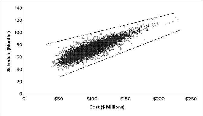
As an example, consider a program for which joint cost and schedule risk is modeled with a bivariate lognormal distribution. Suppose the cost mean is $100 million, the cost standard deviation is $25 million, the schedule mean is 72 months, and the schedule standard deviation is 12 months. The correlation between cost and schedule is assumed to be 60%. Figure 4.3 displays the results of 5,000 simulations from this distribution. Some strange pairs pop up, including mismatched pairs, such as one with a cost equal to $180 million and schedule equal to 60 months. This is the cost and schedule labeled B in the figure. At first glance, it appears that the schedule is shorter than average while the cost is higher than average. Indeed, the chance that the schedule does not overrun is 16%. Only about one in six times will the schedule turn out to be that short, while five out of six times it will be longer than that. On the other hand, the cost is significantly higher than average. In this case, the cost is far in the right tail—above the 99% confidence level. This represents a significant cost overrun that has a shorter than average schedule. In this case, there has been an extreme cost growth event but a much better than average schedule. This rarely happens.

Figure 4.3 Impact of Not Modeling Tail Dependency

As another example, another point on the cloud of simulation outcomes is cost equal to $101 million, while schedule is equal to 114 months. The schedule is much higher than average while the cost is only 1% higher than its average. This is the point labeled A in the figure. An extreme schedule slip has occurred, but the cost is about average. This is also extremely rare. Extreme cost and schedule events should occur together. A significant increase in schedule will increase cost as well, and extreme cost growth is typically accompanied by a big schedule increase. This is the result of the failure to incorporate tail dependency—correlation alone will not account for this.

Figure 4.4 displays the results of 5,000 simulations from a joint distribution with the same lognormal distributions as the cost and schedule distributions before but with tail dependency incorporated.

Figure 4.4 Impact of Modeling Tail Dependency

The incorporation of tail dependency fixes the issue. When an extreme cost or schedule event occurs, the other moves in tandem. The copula is a widely used tool in the financial and insurance industries but is rarely discussed in other projects. Wider adoption of this modeling technique and the inclusion of tail dependency will result in more realistic cost and schedule risk analyses.

EVOLUTION OF S-CURVES THROUGH PHASES

I was the lead estimator on a team that conducted cost and schedule risk analyses for a large mission. Many of the factors necessary for a credible cost risk analysis—including correlation—were included. We incorporated significant amounts of variation in our models and incorporated the impact of technical risks. Despite this, the final budget for the project was 75% greater than the 50% confidence level developed less than three years prior. See Figure 4.5 for a graph of the S-curve evolution over time compared to the final budget. Over a three-year period, the cost risk analysis was updated several times. With each iteration, the S-curve widened and moved to the right. The cost growth was due to a host of factors, some internal to the project and some external. Internal factors included early overestimation of heritage. Two of the three major elements were supposed to be modifications of existing hardware but turned out to be completely new designs. Another internal factor was underestimation of the technological challenges. External factors included funding delays and two major schedule slips.

Figure 4.5 Development S-Curve Evolution for an Actual Project

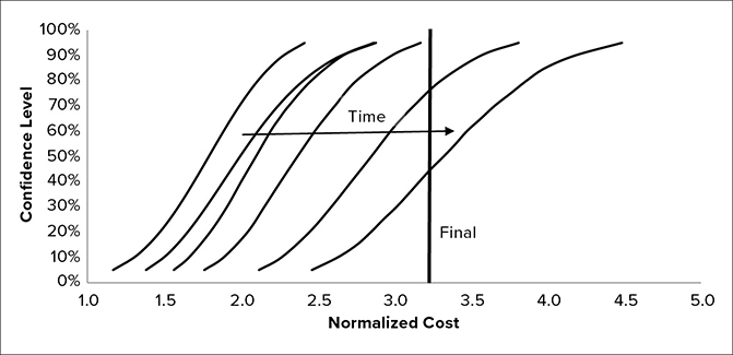
Despite incorporating credible methods in our analysis, the final budget was not even on the original S-curve. This is partly due to the estimate reflecting project inputs. This was not an independent estimate but rather a project estimate. As such, it reflected the project’s optimistic assumptions. The last S-curve occurred prior to the final design review, called the Critical Design Review. The project was cancelled a year later. Still early in the project, we found that as the design took shape additional risks were uncovered. This led us to widen the S-curve as time progressed, accounting for a greater increase in understanding of the risks involved. Variation in the model inputs increased after receiving additional participation in the risk identification process from project personnel through the implementation of a risk tracking system. While the actual amount of uncertainty may be greater earlier in the project, the way that risk is measured is actually the reverse. Initial optimism eventually gives way to reality.¹⁴ Indeed, an independent cost risk analysis during the middle of this process had a wider range than the one we produced for the project. Its 90% confidence level was greater than the final budget.

IT WORKS IN PRACTICE, BUT DOES IT WORK IN THEORY?

Plato is widely considered to be the most influential philosopher on modern Western thought. Plato founded an academy, which was the precursor to the modern university and is the origin of the word academic. Plato believed that what we see in the real world is a reflection of a true ideal.¹⁵ Plato’s influence is much deeper than just providing academia its name. His emphasis on abstract ideals in his academy is the model that has shaped modern academic thought in Europe and America. This emphasis on abstractions of real objects led to the triumph of theory over empirical reality.

Milton Friedman was one of the most prominent economists of the twentieth century. Friedman had a significant impact on economics. His theory of positive economics,¹⁶ in which he stated that the assumptions in economics need not make sense, as long as they yield accurate predictions, has been called the “most influential work on economic methodology” of the twentieth century.¹⁷ This would be all well and good if everyone measured the accuracy of their predictions to make sure their simplifying assumptions did not lead their models astray. However, some have used the idea of positivism as a license to make simplifying assumptions that yield elegant mathematical theories, without worrying too much about the business of prediction. William Baumol was a leading economist of the twentieth and early twenty-first centuries who was an exception to the lack of concern for prediction among economics professors. Baumol did some part-time work as a management consultant, where he discovered that the conventional economic theory assumption that firms seek to maximize profits is not true. Rather, firms seek to maximize revenues subject to a minimum profit constraint.¹⁸ Unlike conventional economic theory, this explains the drive in the modern economy to large firms and the relative lack of competition.¹⁹ Baumol was also known for correctly predicting back in the 1960s that the cost of both healthcare and education would rise higher than inflation.²⁰

Unlike Friedman, Baumol believed that while “ridiculous premises may sometimes yield correct conclusions,” this is the result of “spurious correlations.”²¹ Correlations like these look good on paper but are worthless in prediction. For example, between 2001 and 2009, the correlation between Brad Pitt’s earnings and the average amount of ice cream consumed by Americans was 91.4%. Another example is that, between 2002 and 2010, the correlation between the annual number of tornadoes and the number of shark attacks in the United States was 77.4%.²² Unlike shark attacks and ice cream sales at the beach, there is unlikely to be even an underlying common cause for these two different pairs of events.

I majored in economics and mathematics in college. I was exposed to Friedman’s theory of positive economics by one of my economics professors. This was during the fall semester around the time of the annual football game between the University of Alabama and Auburn University. Known as the Iron Bowl, this game is the biggest annual sporting event in the state of Alabama. One of my neighbors had two tickets to the game that she could not use and was willing to give them away. As she could have easily sold these tickets for a hefty amount, I informed her that her behavior was irrational. The economic assumption of rationality, which states that people choose actions that maximize their self-interest, is a key tenet of economic theory. As this example shows, economic theory often clashes with real-world reality.

The emphasis on theory divorced from reality applies not only to academia but also the current state of practice for risk analysis. The conventional wisdom on cost and schedule risk recognizes that it is not static over time. It evolves as the project matures. Uncertainty shrinks over time. There is a cone of uncertainty that reduces as the project progresses from start to completion. Uncertainty is greatest at the start of a project. This shrinks over time as risks are either encountered or avoided. At the end of development, there is no uncertainty. This is reflected as the cone of uncertainty as illustrated in Figure 4.6.

Figure 4.6 The Cone of Uncertainty

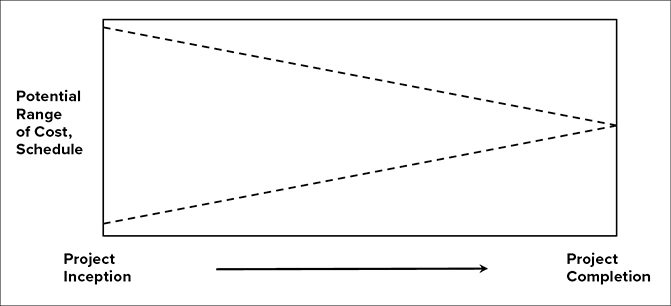
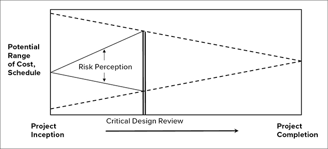
The cone of uncertainty is conceptually correct. However, like many Platonic ideals, it is useless in practice because it ignores how risk is perceived and measured. Rosy optimism prevails early in a project’s life cycle, with assumptions of a high degree of heritage and few known risks. While the risk may be greatest at the beginning of the program, the perception is that risk is low. Many risks are assumed away because of inherent optimism. For example, once a project starts, engineers determine that there is a serious technical issue that requires a design fix. The identification of these kinds of risks widens the perception/recognition of risk as they are discovered, leading to an increase in the amount of perceived uncertainty. Eventually, the perceived risk matches the reality; then both narrow close to project completion after most of the risks have been realized or avoided. The way in which risk is measured in practice does not appear to be a cone at all but is more like a diamond. Risk perception starts out narrow, widens to a peak somewhere between the detailed design review and integration, and then eventually narrows as the project approaches completion. See Figure 4.7.

Figure 4.7 Risk Perception vs. Reality

As the physicist Niels Bohr once said, “Prediction is very difficult, especially about the future.”²³ Explaining the past is much easier than predicting the future. However, we confuse our ability to explain the past with our capability of predicting the future. This leads to overconfidence in predicting, which results in an underestimation of risk. Nassim Taleb, author of The Black Swan, calls this the “narrative fallacy.”²⁴ The need for control leads to ignoring risk and uncertainty. Programs that use cutting-edge technologies are fragile in that the realization of seemingly small risks can have big consequences.²⁵ In the 1970s, the petroleum engineer Ed Capen recognized that technically trained people such as engineers do not understand uncertainty and that there is a universal tendency to understate risk. Survey studies were conducted to assess people’s confidence about their knowledge on a variety of topics. The result found that there was an “almost universal tendency” to underestimate uncertainty because people “overestimate the precision of their own knowledge.”²⁶

One measure of uncertainty in statistics is called a confidence interval. A statistical procedure, such as sampling, that is used to produce a confidence interval will include the parameter of interest with a specified probability. For example, a 90% confidence interval for a parameter is one that will contain the parameter for 90% of sampled intervals. A paper Capen published in the Journal of Petroleum Technology in 1976 included the results of extensive surveys of confidence interval estimates by individuals. More than 1,000 individuals were asked questions about a variety of topics, all of which had a quantitative answer. One such question was “What was the census estimate of the US population in 1900?” People were asked to provide not a single best answer but a 90% confidence interval around their best estimate. Students of American history might provide tighter bounds, while those with less knowledge of the subject might have wider bounds. If people were able to quantify their uncertainty about the answer accurately, 90% of the ranges provided should contain the correct answer. The results indicated that these 90% confidence intervals were more like 40% confidence intervals. People overestimated their knowledge and underestimated their ignorance.²⁷ The same underestimation of uncertainty holds true today for all projects. (The correct answer to the question about the US population in 1900 is 76 million. Does that seem low to you? I would have estimated it would have been at least 100 million.)

CALIBRATION

One way to correct for early optimism is to calibrate the S-curve to historical cost and schedule growth data. There is a significant amount of risk that no one can predict in advance, especially Donald Rumsfeld’s unknown unknowns. We know they will occur for every project, and we can predict their future probability of occurrence in the aggregate based on the historical track record of cost growth. The same notion is used in calculating risks to establish insurance premiums.²⁸ Calibration is simple. Risk can be calibrated in a variety of ways—it can be done with as few as two inputs. For example, risk can be calibrated to an initial estimate assuming a percentile for the point estimate and a variation about the point estimate.

Applied to the project illustrated in Figure 4.5, an S-curve based solely on the initial estimate and calibrated to empirical cost growth data was much more realistic than the more sophisticated and detailed risk analysis that involved uncertainties on the inputs, uncertainty about the CERs, correlation, and Monte Carlo simulation. See Figure 4.8 for an illustration. The final budget is slightly below the 70th percentile of the empirically calibrated S-curve.

Figure 4.8 Empirical S-Curve Compared to the Final Budget

Even with best practices like correlation incorporated, S-curves are still not wide enough to be realistic. Risk is greatly underestimated in the early stages of a project. Calibrating the risk to historical cost and schedule growth variations is an objective way to overcome this problem. It tempers the inherent optimism in the early phases of a project before most of a program’s risks are discovered or admitted. Calibration to empirical cost and schedule growth data is a way to correct for this.²⁹ Cost and schedule growth is risk in action. By examining historical cost growth, we can develop methods for calibrating risk to make it realistic.

I have witnessed two types of risk analysis in my career. One I call the naive approach. This is a simple analysis that does not incorporate the best practices discussed in this chapter. The naive approach often includes limited risk ranges, does not incorporate correlation, and generally ignores most sources of uncertainty. Even when risk analysis is conducted, the naive analysis is the most common type I have encountered. As an example of the naive approach, I once reviewed a project for schedule risk analysis that had extremely tight, unrealistic risk bounds. For this analysis, the planned schedule was several years long, but the range from the 5% confidence level to the 95% confidence level was only two weeks. That is, 90% of the uncertainty was captured by a two-week period. Any program delay would cause the total schedule to shift by more than that amount. An accident on the shop floor, a loose screw found in test hardware, a funding delay—any of these events by itself would cause the schedule to slip by at least two weeks. The probability of predicting the schedule within a two-week window is zero. The analyst had done a detailed analysis of the schedule, inputting uncertainty on the durations of individual tasks, and then using a Monte Carlo simulation to aggregate the risks. However, the variations were all assumed to be independent. Also, as we mentioned earlier, schedule risk is aggregated differently than cost risk. Cost is broken down into a set of elements. Risk is assessed for those items, and then those values are added. When it comes to schedule, you cannot add everything—there are tasks that occur in parallel. This must be treated differently than addition. The schedule analyst also did not correctly account for this, which further contributed to the narrow range of the schedule prediction.

How Much Risk Is Realistic?

To discuss how much risk is realistic, we need a notion of relative risk, which allows us to compare risk between projects regardless of their sizes. Recall that the amount of cost risk for a project is often characterized by the standard deviation. The mean and median are measures of central tendency for a distribution, and the standard deviation measures the spread around the mean or median. The absolute spread around the center of the distribution varies in accordance with the size of the project. For example, the standard deviation that results from the cost risk analysis of a small project can be measured in millions or tens of millions of dollars, while that derived from a cost risk analysis for a large project will likely be measured in hundreds of millions of dollars, a difference of at least an order of magnitude. A way to compare risk across projects when the absolute magnitude differs greatly is to examine the relative amount of risk. Suppose one project has a standard deviation equal to $100 million, while another has a standard deviation equal to $10 million. The first project has a mean equal to $1 billion, while the other has a mean equal to $10 million. Calculating the ratio of the standard deviation to the mean provides a measure of relative risk. This ratio is called the coefficient of variation. The larger project has a standard deviation that is 10% of the mean, so its coefficient of variation is equal to 10%. The other project has a standard deviation that is equal to the mean, so its coefficient of variation is equal to 100%. Since the standard deviation is in the same units as the mean, the coefficient of variation is a scalar. A scalar is a unitless measure that allows for comparison of the relative risk among projects regardless of dollar value. Although the cheaper project has a lower standard deviation, it is relatively riskier than the more expensive one, as measured by the coefficient of variation.

For a variety of projects, including aerospace, weapons systems, roads, tunnels, chemical processing plants, and information technology, the median coefficient of variation exhibited in cost growth data for a variety of projects is 92%.³⁰ See Table 4.2 for a list of coefficients of variation implied by cost growth data for 12 different types of projects.

Table 4.2 Comparison of Coefficients of Variation Implied by Cost Growth Data

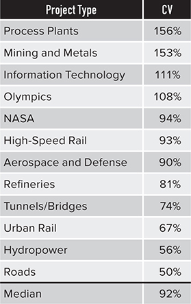
The values in Table 4.2 are much higher than are typically used in cost risk analysis. The values in cost risk analyses often range from 5% at the low end to 30% at the high end. However, the true amount of risk realized in the past as reflected in cost growth data is much higher. The coefficients of variation implied by schedule growth data are just as high as for cost growth, and in many cases even higher.

Comparing Reality with Current States of Practice

The naive approach significantly underestimates risk, as evidenced by historical cost and schedule growth data. The second type of risk analysis, which I refer to as standard, is one I have often produced. Correlation is included and appropriate distributions are used to model risk. However, standard risk analysis often suffers from being anchored to the project manager’s optimism. It incorporates as much uncertainty as the project manager is willing to perceive at that point in time.

Figure 4.9 provides a comparison of these two approaches, along with a comparison of a calibrated, realistic risk analysis based on cost and schedule growth data. These are displayed as ranges from the 5% confidence level to the 95% confidence level.

Figure 4.9 Comparison of Realistic vs. Standard and Naive Practice for Cost Risk Analysis

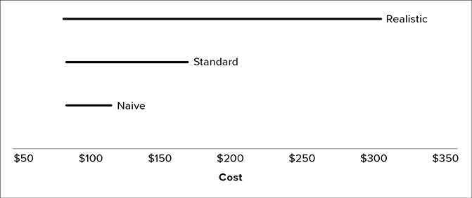
The examples in Figure 4.9 are for a program with a point (riskless) estimate equal to $100. For the naive estimate, the range is $87–$118, 13% below the project estimate and 18% above. This is unrealistic. For most programs, a couple of minor events, such as schedule slip and a single integration issue, can lead to more than 30% cost growth. The amount of reserves needed to fund to the 95% confidence level is only 18% more than the point estimate.

For the standard estimate, the range is $87 to $171. The amount of reserves needed to achieve a 95% confidence level is 71% above the point estimate. This is a healthy amount of reserves for a development program and more than I have ever seen a project set aside for contingency. The standard approach is more realistic. It will be conservative for a low-risk program and may be adequate much of the time. However, it is still less than experienced on average by historical development programs.³¹ The range for a risk estimate calibrated to real cost growth is $85 to $305. To achieve a 95% confidence level will require 205% reserves.

To convince the skeptical that the coefficient of variation implied by historical cost growth is a realistic approach to risk, we compare it and the other two approaches to see how well they would have done in measuring risk for the 10 historical projects discussed earlier in the chapter. See Table 4.3.

Table 4.3 The Number of Missions for Which the 90% Confidence Levels Are Greater Than the Actual Cost

In Table 4.3, we find that the naive approach, much like current practice, produces the opposite of what is expected. For only one of the missions is the actual cost less than the 90% confidence level. The standard approach is better, but still falls short of reality—for only five missions is the actual cost less than the 90% confidence level. This is better than the naive analysis, but the probability of five or fewer projects being less than the 90% confidence level is less than one in 600. One in 600 is still not credible. The realistic case is what is expected. For 9 of the 10, the 90% confidence level is less than the actual cost.³² Also, the range is not so large that all missions are within the range, which means the bounds are not overly wide.

Figure 4.10 provides a similar comparison based on schedule growth data. Schedule risk is displayed as a range from the 5% confidence level to the 95% confidence level.

Figure 4.10 Comparison of Realistic vs. Standard and Naive Practice for Schedule Risk Analysis

The examples in Figure 4.10 are for a program with a point (riskless) estimate equal to 60 months. For the naive estimate, the 5%–95% confidence level range is 55 to 65 months, 8% below the project estimate and 8% above. This is unrealistic for most projects. Relatively minor changes can delay the schedule by more than six months, more than the 95% confidence level on the S-curves. The standard schedule risk estimate ranges from 51 months to 98 months. The amount of time needed for a 95% confidence level is 63% higher than the point estimate of the schedule. This is much more realistic than the naive approach, but according to schedule growth history, the 95% confidence as modeled is more like an 80% confidence level. The realistic schedule risk estimate ranges from 54 months to 146 months. The 95% confidence level is 140% more than the baseline schedule.

Unfortunately, in my experience, the naive approach is about as much risk as most managers are willing to bear. The standard approach, even though it is more realistic, is often unpalatable for decision makers. The realistic risk would cause most project managers to choke upon seeing the results and their implications. However, as we will see later, even funding to a 90% confidence level does not consider the big risks that program managers need to prepare for, as setting funding and schedules using confidence levels ignores the risks in the right tail of the uncertainty distribution.

MEDIOCRISTAN VS. EXTREMISTAN: HOW BIG ARE THE TAILS FOR COST RISK?

As discussed in the previous chapter, there are stark differences between phenomena that belong to Mediocristan as compared to those that belong to Extremistan. Recall that Mediocristan is the realm of mild variation. Gaussian distributions belong there. Examples are variations in human height and life span of humans. Phenomena that belong to Extremistan are those that exhibit extreme variation. Examples are losses due to natural disasters and fluctuations in stock market prices.

If cost and schedule for projects belong to Mediocristan, it has significant implications. In a world in which costs have limited variation, they are easy to predict. There is also a pronounced portfolio effect. This makes it easy to reduce the limited risk of a single program even further by combining it with other programs to achieve a portfolio effect. In such a world, we can fund projects to percentiles slightly above the mean and achieve high confidence levels for an entire organization.

One of the rationales for using the Gaussian distribution in cost and schedule estimating is the central limit theorem. This states that if independent, identical distributions are added, the sum will, in the limit, approximate a Gaussian distribution. The only catch is that the variations must not be too extreme. The requirements are that the distributions are independent, none exhibits extreme variation, and the total is the sum of “many individually negligible components.”³³ The central limit theorem has been the rationale for modeling many phenomena as Gaussian that are not Gaussian distributed, including cost and schedule. The idea is that even if the lower-level elements are not Gaussian, in aggregate they will be due to the convergence of sums to Gaussian.

As applied to project cost and schedule uncertainty, there are multiple issues with the application of the central limit theorem. One is that it applies at “the limit,” which occurs when we add infinitely many random variables together. The real world does not operate “in the limit.” In practice, any total will necessarily be the sum of a finite number of random variables. For highly specialized projects, a limited amount of directly applicable data is available. In many cases, less than 10 directly applicable historical data points exist. The central limit theorem requires that everything be independent, but there are a multitude of established interdependencies within and among projects. Earlier in the chapter, we explained why all programs have some positive average correlation and a higher level than is commonly believed. The central limit theorem also requires finite standard deviation. There is some evidence that for cost this may be infinite. Even if the standard deviation is finite, for the central limit theorem to apply, no one project can dominate the total standard deviation. However, it is often the case that there will be a series of programs with small overruns. Then, a project with a huge amount of cost or schedule growth will occur. Thus, when it comes to cost and schedule estimating, all the assumptions required for the central limit theorem to hold are suspect. Not enough elements are summed to be close to the “limit,” projects are not independent, and the standard deviation is not well-behaved.

Even if the Gaussian distribution is not representative of cost risk, the lognormal seems to be a good alternative much of the time. However, if the tails of the distribution are even riskier than the lognormal, the analysis is trickier. If this is the case, there are some serious implications for how analysis is done, as many traditional analysis tools, such as regression, are based on limited variation. I have compared fitting the tail of cost growth data to lognormal and Pareto-type distributions. I have found the lognormal distributions fit the tail better in some cases. However, in others, a Pareto-type power law distribution prevails.

The argument for the lognormal is that changes in costs over time are proportional to prior costs. Cost is more likely to increase than decrease over time, as we have discussed. When we talk about cost changes, we almost always mean cost increases. Cost increases often do not result in funding increases in the short term due to funding constraints. Thus, cost increases will result in longer schedules. Longer schedules imply a longer period in which the personnel devoted to a project will charge to that project. Larger projects have more personnel assigned to a project, meaning that increases in cost will result in a proportional increase in cost. This process generates a lognormal distribution.³⁴ This assumption is not robust. Only a slight change to this generative model is needed to turn the lognormal into a power law. An additional assumption that cost has a lower bound is all that is needed to cause this change.³⁵ This is reasonable since, once a project begins detailed work, cost decreases are unlikely. Almost any change, apart from cutting scope, will result in cost and schedule increases. The only way to effectively change a project without increasing cost is to cut requirements.

One analysis I conducted for 133 NASA missions indicates that the right tail follows a power law that indicates finite mean but infinite standard deviation.³⁶ For this data set, a power law (Pareto) distribution for the right tail was a better fit than a lognormal distribution. This evidence puts cost growth in the territory of Extremistan.

As is evident from Table 4.4, the chance of extreme cost growth is remote for the lognormal. The probability that a program would experience 1,000% cost growth is practically impossible for a lognormal, while for a Pareto the chance is only a little less than 1%. The Pareto may be conservative, but the lognormal does not provide realistic odds of extreme growth. For example, the James Webb Space Telescope is one program that is not included in the 133 data points. This next-generation space telescope, discussed in the Introduction, is a successor to Hubble and truly cutting-edge technology, as was Hubble when it was launched. Like Hubble, it has also experienced significant cost growth. As of early 2020, the James Webb Space Telescope had grown by more than 500%, more than any program in the database used in the analysis that was used to generate Table 4.3. The lognormal predicts the chance of this amount of cost growth experienced by this project to be 1 in 2,940, while the chance with a Pareto is much higher, 1 in 70. If we were to add this data point to the database, it would be one of 134 data points. So the empirical probability would be between that predicted by the Pareto and lognormal but closer to the Pareto than the lognormal. This kind of extreme growth is not limited to aerospace or defense projects. A notable example of a high-priority project is the Sydney Opera House, which, as discussed in the earlier chapters on cost growth, increased in cost by a factor of 14. To meet an aggressive schedule, funding poured in to support National Missile Defense in the 2000s. The cost to develop the Suez Canal in the 1860s increased 20-fold from the initial plan. The actual cost for the Concorde supersonic airplane was 12 times the initial cost.³⁷ The cost for the new Scottish Parliament built in the early 2000s was 10 times the initial estimate.³⁸

Table 4.4 Comparison of Lognormal and Pareto Tails for Modeling Cost Growth

The case for the lognormal is buttressed by the fact that the wild risks of the stock market and natural disasters cannot be easily mitigated, while more traditional projects are more easily controlled. A project manager can cut scope or implement measures to improve project performance. Also, projects that experience extreme cost and/or schedule growth will likely be cancelled. The counterargument is that some of the time a project will be high priority. Even when it experiences extreme cost growth, a high-priority project will not be cancelled. Instead, the schedule will slip and/or funds will be reallocated from other lower priority programs to pay for the program. This occurs for projects that not only double in cost but increase by a greater factor, such as four or more. In some cases, technology is so cutting edge that little can be done to reduce costs. It will cost what it costs. All these are examples of publicly funded projects. (Even though the Concorde was a commercial aircraft, its development was supported with government subsidies.³⁹) Private firms would likely go out of business if costs grew by these amounts. For example, FoxMeyer, the pharmaceutical wholesaler mentioned earlier, went bankrupt when its planned implementation of a new enterprise resource planning computer system increased in cost by less than 100%. Also, Airbus’s A380 aircraft was a consistent money loser for the company, and its development costs are believed to have doubled from initial plans.

Even though schedules exhibit significant variation in absolute terms, there needs to be extreme variation on a percentage basis to belong to Extremistan. For example, the Sydney Opera House schedule lengthened from 4 to 14 years. In percentage terms, that is a 250% increase. Using Table 4.4 as a comparison, the lognormal models that level of increase as relatively rare (one in 94), while it is four times more likely with a Pareto. A Pareto also estimates 1,000% growth as not uncommon, on the order of one in 156 projects, while for the lognormal it is likely to never occur (one in 100,000). An order of magnitude increase would mean an initial four-year plan would stretch to 40 years or a 10-year schedule would slip to 100 years. These kinds of increases are extremely unlikely. This puts schedule in the realm of Mediocristan. Schedule is not Gaussian, but a lognormal should be sufficient to model time risk, even in the right tail.

Power law distributions have three categories. In one, both the mean and standard deviation are finite. For the second, the standard deviation is infinite, but the mean is finite. In the third, both the mean and standard deviation are infinite. Power law distributions are typically used to model phenomena in which at least one of these first two moments is infinite. See Table 4.5 for a comparison of three Pareto distributions. These have drastically different percentiles, although all three have significant risk. The relative difference between the 70th and 95th percentile for the thinnest-tailed Pareto is a factor of almost four. For the finite mean, infinite standard deviation version, the difference is similar. The relative differences are an order of magnitude greater for the infinite mean, infinite standard deviation Pareto. Also, the 70th percentile is almost an order of magnitude larger for the latter Pareto. The kind of risk exhibited by an infinite mean, infinite standard deviation Pareto is the type of risk seen in box office returns for cinematic films. Most projects do not display this degree of risk. Imagine a large $5 billion nuclear plant or missile development project that suddenly grew to cost $5 trillion.

Table 4.5 Comparison of Percentiles for Three Different Pareto Distributions

If cost growth for most projects indeed follows a Pareto, it is the type with finite mean. This makes predicting the cost of these systems difficult. However, there is still more capability to effectively forecast than cases where the mean is infinite. The answer to the question, “Does cost risk follow a lognormal or a Pareto distribution, at least in the tails?” is, in many cases, “It depends.” My hypothesis is that the lognormal applies to most private and public projects. The exception is those projects that have poor planning or execution and that are high enough priority to avoid cancellation once costs spiral out of control. Some of the projects we mentioned with extreme cost growth used advanced technologies, like the James Webb Space Telescope and the Concorde supersonic airplane. The initial planning was poor because it did not adequately account for the difficulty in maturing the critical technologies required. This resulted in extremely optimistic estimates. The issue with the Scottish Parliament building was optimistic initial estimates and design changes during construction. Some of the increase was due to additional security requirements added after the 9/11 terrorist attacks in the United States, but the project was essentially given a blank check, and no one had the discipline to keep requirements from growing.⁴⁰ If costs increase by a significant amount, a project that is not high priority will be cancelled. Otherwise, in those instances where a public project is high priority and uses cutting-edge technologies, the right tail for cost risk follows a power law. This issue is partly a matter of incentives. Without some motivation to keep costs low, costs can quickly balloon by a factor of 5 or 10, and still fail to meet objectives. Extreme cost growth for projects is often a matter of a lack of incentives, a subject we will discuss in more detail in Chapter 8.

The one exception of the application of the lognormal in private projects is software and information technology. There is some evidence that these projects have fat tails.⁴¹ The relationship between software cost and size exhibits diseconomies of scale. In percentage terms, the cost of a software project grows more than proportionally to its scale. For example, if the size of the project grows by 50%, the cost will grow 60% or more. Optimistic requirements during the planning process will lead to correcting the initial scale during development. This will lead to large cost increases, possibly tipping the risk into the realm of Extremistan. Approaches to software development have changed over the years to cope with the issues related to complexity. The Agile approach has the promise to potentially reduce cost.⁴² The outstanding question is whether it can reduce risk as well.

Evidence of similar extreme variation in financial data arose in the 1960s. Benoit Mandelbrot had applied his analytical framework to financial data and had found that the Gaussian distribution was not a good fit. Instead, it exhibited extreme variation, particularly infinite standard deviation. One of Mandelbrot’s early applications of his PhD dissertation topic mentioned in the last chapter was to financial markets in the early 1960s. He found that prices in markets like cotton did not fit a Gaussian distribution but that they had much more variation than would be expected from a Gaussian or even a lognormal. This led to a significant degree of controversy in the academic community for finance, as the foundation of the theory of finance was based on Gaussian and lognormal distributions. The MIT economist Paul Cootner wrote in 1964 that “Mandlebrot, like Prime Minister Churchill before him, promises us not utopia but blood, sweat, and tears. If he is right, almost all of our statistical tools are obsolete … almost without exception, past econometric work is meaningless.”⁴³ Mandelbrot’s ideas were resisted and eventually rejected for more conventional models. The early 1970s hearkened more financial tools, like the Black-Scholes model of option prices, that rested upon Gaussian and lognormal distributions, pushing Mandelbrot’s ideas into the background. While they realized there was evidence for extreme variations, in their view the Gaussian distribution was good enough.⁴⁴

If risk is not lognormal, but fatter tailed, it has significant implications for cost estimating. In the case of extreme risk, point estimates are not useful from a predictive standpoint. Traditional cost estimating practice, including cost risk analysis, uses methods designed for mild variation. Detailed discussion of the implications is beyond the scope of this book. I mention it here to note that for some projects, traditional tools should not be used to estimate cost. This includes standard regression analysis. Fortunately, there are plenty of alternatives, such as basing estimates on absolute deviations rather than squared deviations. There is a plethora of tools available in the burgeoning field of machine learning that do not rely on distributional assumptions.

SUMMARY AND RECOMMENDATIONS

There is a systematic tendency to underestimate risk. Blindness to risk is a human tendency. In Shakespeare’s play Hamlet, the title character says to his friend Horatio that “there are more things in heaven and earth, Horatio / Than are dreamt of in your philosophy.”⁴⁵ Projects suffer from Horatio’s defect. Numerous sources of risk for cost and schedule estimates exist. If a statistical model is used to predict cost and schedule, there are uncertainties in the inputs to the model. Also, the models themselves only explain a portion of past variation in cost and schedule. If an analogy is used, the similarity of the analogy to the program being estimated is uncertain, as are any adjustments that must be made to the analogy to obtain a program estimate. Programs have internal issues, such as the technologies used for the program. Incorporating new technologies into a program is inherently risky. The integration of existing technologies in new configurations also has substantial risk. The biggest risks are those external to the program. However, as projects do not plan for most of these, risk is underestimated.

The results of past cost and schedule risk analyses are not tracked to measure their accuracy. This has led to no improvement in the accuracy of the application of risk analysis over time. We provided a sample of 10 missions and showed that for 8 of the 10, the actual cost exceeded the 90% confidence level for the cost risk estimate. For the two missions with schedule risk estimates, one of them was 2.8 times greater than the 90% confidence level.

The cause of the underestimation of risk is seen to be the risk perception early in a program’s life cycle. Cost and schedule estimates and risk analyses for them are influenced by program office assumptions. Typically, early in a program, the intent is to use existing technologies and leverage existing designs as much as possible. However, as a system design matures, the true risks are revealed (and in some cases admitted). This leads to wider risk ranges that are more realistic. As a result, the ideal “cone of uncertainty” looks more like a diamond than a cone. The amount of risk perceived is tiny at project inception. This increases as risks are discovered or can no longer be ignored. The perceived risk eventually expands until it matches reality. Then both perceived and actual uncertainty narrows as risks are realized, avoided, or mitigated.

The bottom line is that risk is not modeled accurately. The use of sophisticated tools and advanced methods is not sufficient to avoid this problem. The solution to the issue of risk perception is calibration to empirical cost and schedule growth data. This is an objective measure that can avoid the taint of early program optimism. Even if it is not used as the primary risk methodology, it should be used as a cross-check to verify that early risk analysis is realistic. Even with calibration, it is possible that we are missing the boat if we are suffering from another perception issue, which is that we think projects could have mild variation when they could experience extreme variation.

The argument for mild variation is that programs will be cancelled if they experience extreme cost growth. There is a check to ensure things do not get out of hand, unlike with other phenomena that have wild variations, such as natural disasters and stock prices. Also, private firms may go bankrupt once cost growth gets out of hand. Publicly funded projects do not have this constraint. Public projects that are good candidates for extreme cost and schedule growth are those that require technology development and are high priority.

When I was a child, my family had a small, mischievous dog named Tessie. Whenever she did something that caused my mother to reprimand her, she would turn her head away. Tessie was purposely avoiding the reality of my mother’s reproach. In a similar manner, project managers often ignore risk. To borrow a phrase from the film A Few Good Men, they “can’t handle the truth.” This needs to change. Project managers must develop a proper appreciation for risk if they want to be successful and to avoid the problems that occur when unplanned for cost and schedule risks are realized. Managers and analysts both need to honestly assess projects to determine if they are candidates for extreme cost and schedule growth.