CHAPTER 5

The Portfolio Effect and the Free Lunch

The Limits of Diversification

Most people know that the Wright brothers invented the motor-operated airplane and that Alexander Graham Bell devised the telephone. However, many people do not know that a more modern innovation that has had a significant impact on people’s lives started with a single individual named Harry Markowitz. An investment portfolio is the total of all the investments owned by a single individual or organization. If you invest in the stock market, have a 401(k) at work, or use the services of a financial adviser, you likely have such a portfolio. Your investments are in a portfolio to take advantage of diversification. Before the 1950s, conventional wisdom held this was not a good strategy. Most financial research was focused on identifying the single best stock and investing all your money in that company. The thinking up to that point was encapsulated by Mark Twain in his novel Pudd’n’head Wilson, “Behold, the fool saith, ‘Put not all thine eggs in the one basket’—which is but a manner of saying, ‘Scatter your money and your attention;’ but the wise man saith, ‘Put all your eggs in one basket and watch that basket!’ ”¹ The economist John Maynard Keynes considered diversification in a large pool of investments, about which the investor had little direct knowledge, to be a “travesty.”² Prior to 1950, the leading publication on investing was The Theory of Investment Value, a PhD thesis written by John Burr Williams, who had prior practical experience working as a securities analyst. In his dissertation, Williams showed how to estimate the value of a stock by projecting the company’s long-run dividend. He recommended finding the single stock with the highest expected return and buying only that particular stock.³ A best-selling investment book of the first half of the twentieth century, The Battle for Investment Survival, stated that “the intelligent and safe way to handle (investment) capital is to concentrate.” The author of this book, who worked on Wall Street, wrote that if an investment is “not worth following to the limit, it is not worth following at all.” Diversification was described as “undesirable” and “an admission of not knowing what to do and an effort to strike an average.”⁴

Markowitz developed portfolio theory in a paper published in 1952.⁵ He had noticed that prior research on the selection of stocks and bonds focused solely on expected return. Markowitz realized it was important to consider the spread around the mean return and introduced the consideration of risk. One stock may be growing faster in price than another but, if it is also more volatile, that should be considered as well. For example, a technology stock may have more growth potential than the stock of a company that makes soft drinks or razor blades. However, technology stocks, especially of small, less established companies, are much more volatile and hence riskier. Markowitz noted that the combination of a variety of stocks held in a common portfolio is less risky than the most volatile individual member.⁶ This is one of the benefits of diversification. Another is that investing in a broad variety of stocks makes it less likely to miss out on big gains. In investments such as stocks, large gains and losses are possible, depending on the level of risk an investor is willing to take. A stock market investor who is not using leverage can lose no more than he or she invests but has the potential for tremendous gains. For example, during the period 2000-2019, the price of Apple stock shares increased 10,000%. If an investor did not diversify sufficiently to have a stock like this in their portfolio, their overall return was likely significantly lower over this time period. The benefits of diversification led stock pundit Jim Cramer to tout it as the “only free lunch on Wall Street.”⁷

THERE AIN’T NO SUCH THING AS A FREE LUNCH

The notion of a free lunch dates to the nineteenth century. American saloons would offer customers a “free lunch” if they purchased an alcoholic drink. The food offered in the free lunch would be over-salted, leading customers to buy multiple drinks. Drink prices at such establishments were also higher than those that did not offer a “free lunch.”⁸

The nineteenth-century German philosopher Johann Fichte discussed the evolution of ideas as a debate between opposing forces. In Fichte’s view, every thesis would give rise to an opposing antithesis. Ideally these two contradictory ideas would eventually be reconciled into a synthesis.⁹ We see an example of the thesis-antithesis-synthesis cycle in our own development as we mature. When we are young, the idea our parents know everything is the thesis. When we rebel against this authority as teenagers and young adults, we think we know everything, which is an antithesis to the original thesis. Eventually our views moderate, and we synthesize these two views, learning to appreciate our parents’ advice as well as our own judgment.

British economist John Maynard Keynes became famous during and after the Great Depression for advocating government intervention to stimulate the economy during a downturn. Keynes’ ideas have been highly influential in government economic policy in America and Western Europe, and have been primarily associated with big government policies. Libertarian writers and free market economists popularized the phrase “there ain’t no such thing as a free lunch” as an antithesis to Keynesian economic policies. The conservative counterpoint to the government’s meddling in the economy is that while fiscal stimulus may seem like free money, it must come at some cost. This tension between the ideas of government intervention and free market economics remains in American politics to this day.

Two individuals were key to making “there ain’t no such thing as a free lunch” a common phrase. One was best-selling author Robert Heinlein, one of the pre-eminent twentieth-century science fiction writers. Along with Isaac Asimov and Arthur C. Clarke, he was one of the top three early science fiction writers. Several of his books were made into films, including Starship Troopers. He coined several phrases that were popular at one point or another, including “pay it forward,” the basis for a film of its own in the 1990s. Heinlein was a fiscally conservative libertarian. The phrase “there ain’t no such thing as a free lunch” summarizes his economic philosophy. He made it a central concept of his novel The Moon Is a Harsh Mistress, about a lunar colony’s revolt against rule by planet Earth. Heinlein used it so much in the book that he made it an acronym—“TANSTAAFL.” In this book, he defines it as “anything free costs twice as much in the long run or turns out worthless.”¹⁰ The other person to help make the phrase popular was Milton Friedman, a Nobel Prize–winning economist with a knack for explaining abstruse economic concepts in easy-to-understand language. Friedman was a twentieth-century conservative economist and popular speaker and writer on economics. He believed in free markets rather than free lunches. Friedman was the leading opponent of Keynesian economic policies. Along with Keynes, he was considered one of the two most influential economists of the twentieth century. Friedman was the leader in developing the antithesis to the Keynesian thesis. He believed that government economic stimulus would just lead to inflation and not affect overall employment. As an advisor to President Ronald Reagan, he had a lasting influence on Republican policies. Friedman published a collection of magazine columns and interviews in the 1970s in book form titled There’s No Such Thing as a Free Lunch.¹¹ As we will see, the “no free lunch” principle applies to diversification as well.

THE PORTFOLIO EFFECT

An important facet of cost risk is that budgets are not typically set in isolation. Rather, they are established in the context of multiple ongoing and planned projects. This collection of projects can be considered a portfolio. The risks for these projects are not perfectly correlated with one another, so overall portfolio risk should be less than for any single project. The prevailing thesis is that it is possible to achieve a high level of confidence in the overall budget for an organization while setting budgets for individual projects at a lower level.¹² This portfolio effect is relied upon in setting confidence level policy for programs that consist of multiple projects. Note that this purported effect applies only to cost, not schedule. Cost is fungible. An overrun in one element can be offset by another that underruns. Time is not. An early completion for one project cannot be used to offset a schedule slip for another.

Markowitz’s introduction of the consideration of risk is a landmark achievement. The application has led to the widespread appreciation of diversification in investments. However, Markowitz’s work has some shortcomings that limit its application to project risk management. In his research, the benefits of diversification rely upon the ability to measure risk as the standard deviation. There is no accounting for skewness, which, as we have discussed, is a prominent feature of cost risk. It also relies upon mild variation, such as measured by the Gaussian distribution. However, diversification is important in investing because in a limited risk situation, the wild variation in financial prices means that the returns of a portfolio will be dominated by a single investment, such as Apple.¹³

While based on the idea of investment diversification, the notion of the portfolio effect depends on relative risk and reward. For many projects, the situation is the opposite of that faced by the typical stock market investor. For public endeavors, such as roads or satellites, the gain can be valuable, but it is relatively fixed and can be difficult to measure quantitatively. However, there is a large potential downside in that cost can increase dramatically.

The 80% confidence level is commonly used for funding projects when a quantitative cost risk analysis is conducted. The use of S-curves and percentile funding for financial risk management arose in the banking industry in the 1990s.¹⁴ In the banking industry, the use of confidence levels is called Value at Risk. Other types of projects have adapted this approach.

The Department of Energy, the US government agency in charge of nuclear projects, requires confidence levels in the 70% to 90% confidence level. These are separately required for cost and schedule.¹⁵ For infrastructure projects, when funding levels are based on quantitative risk analysis, funding is at the 50% or 80% confidence level.¹⁶ Public projects in Australia,¹⁷ the United Kingdom’s rail network division,¹⁸ and US transportation projects¹⁹ are among those organizations that regularly fund to the 80% confidence level. Some projects occasionally fund to higher levels. For example, the Niagara Tunnel megaproject was funded to the 90% confidence level.²⁰ The 80% confidence level is also commonly used for establishing schedule reserves.²¹ NASA policy requires funding at the 50% and 70% confidence levels, depending on the project. This requirement is for a joint cost and schedule confidence level, so a 50% joint confidence level is a 50% chance that neither cost nor schedule will exceed the specified cost and schedule.²² Two key differences between the use of confidence levels for establishing funding for banks compared with other projects are the horizon, or period over which risk is considered, and the confidence level used. In banking it is a shorter time period, up to one year, and confidence levels equal to 95% or higher.²³

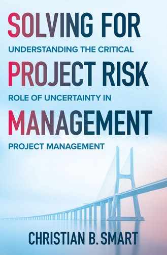
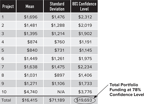
In 2003, the Office of the Undersecretary of Defense for Acquisition, Technology, and Logisitics published a report that noted high amounts of cost growth for defense programs. It recommended budgeting to the 80th percentile. This was much higher than the mean or median that many defense projects had used as a basis for funding recommendations,²⁴ so there was naturally a backlash. A year after the release of the report, a presentation at a symposium illustrated the portfolio effect for a set of 10 notional projects. It showed a substantial savings due to diversification.²⁵ Table 5.1 contains the notional example presented as an antithesis to the recommendation to fund individual projects to the 80th percentile. In Table 5.1, there are 10 mutually independent Gaussian distributions. In this case, an 80% confidence level can be achieved for the full portfolio of 10 missions while budgeting each individual mission at the 61% confidence level. The sum of the 80th percentiles of each individual mission is $16,959. Only $14,720 is required by considering these as a portfolio, approximately a 13% reduction in the total needed to fund to the 80% confidence level for the entire portfolio.

Table 5.1 Example of the Portfolio Effect for 10 Mutually Independent Gaussian Distributions

Analysis of the type provided in Table 5.1 was part of the reason the Department of Defense eventually rejected funding to 80% confidence levels. The idea of a portfolio effect did not just take a firm root in military endeavors, it also quickly migrated to NASA and is now firmly established in all types of projects. Bent Flyvbjerg, Oxford professor and expert on risk for large projects, has stated that funding to the 50% confidence level “is often used to forecast projects in a portfolio of projects, because in this manner on average underruns will compensate for overruns and the portfolio will balance overall.”²⁶

All the aggregation in Table 5.1 can be done with addition because all the distributions are Gaussian. The sum of two Gaussian distributions is also Gaussian. In this example, the analysis is straightforward and there are formulas to do all the calculations. However, this effect is more apparent than real. The analysis in Table 5.1 has at least three issues. One is that cost risk does not typically follow a Gaussian distribution, as we discussed previously. Instead, cost risk is skewed to the right. A second is that projects are rarely independent. The greatest source of risk, Don Rumsfeld’s “unknown unknowns” such as budget cuts and funding constraints, affect all projects, which results in some positive level of correlation among most cost elements. A third issue with the analysis in Table 5.1 is that the risk is vastly understated compared to actual experience. The relative riskiness of the notional projects in Table 5.1 is lower than would be expected from cost growth history, although unfortunately it is in line with the way risk is typically assessed, as discussed in Chapter 4.

Adjusting the Assumptions to Match Reality

I was skeptical of the idea of a portfolio effect for public projects as soon as I learned of it. It could be a natural bias on my part. I am the only child of an only child who was also an only grandchild. My son and I are the only lineal descendants of one of my great-grandfathers. I like to say my family tree is more like a family vine. One of the issues I noticed about the analysis in Table 5.1 is that it did not seem realistic. We adjust it in three ways to make it more faithful to the true amount of risk. First, we change the distribution type. We use a lognormal instead of the Gaussian. The lognormal distribution’s skew models the fact that more can go wrong than can go right and that extreme events are likelier to occur than with a Gaussian. Second, we add a realistic amount of correlation. Third, we assume relative amounts of risk that are derived from empirical cost growth data, as discussed in the last chapter. When we want to aggregate the risks for 10 lognormal distributions, however, we cannot do this analytically. Unlike Gaussian distributions, lognormal distributions do not add. To sum lognormal distributions, we must use a computational technique known as Monte Carlo simulation, as discussed previously. Simulating these 10 projects with the same means as in Table 5.1, the results are displayed in Table 5.2.

Table 5.2 The Portfolio Effect Based on Empirical Data

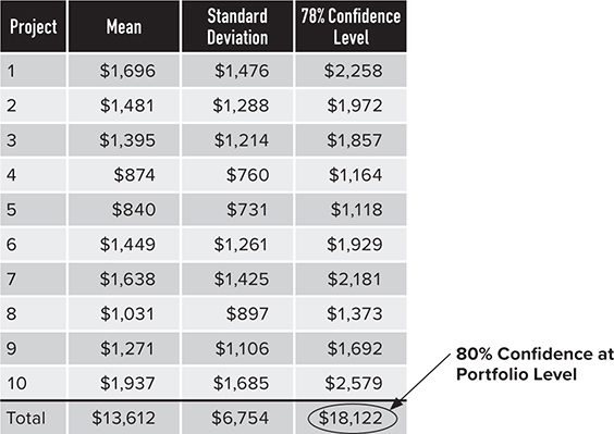
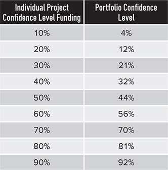
Note that the portfolio effect based on empirical data offers essentially no savings from diversification. To truly fund to the 80th percentile for the portfolio, we must fund each individual project at the 78th percentile. Thus, the portfolio effect is found to be a myth. There ain’t no such thing as a free lunch, and when it comes to confidence level funding, there ain’t no such thing as a portfolio effect, either. Reliance by policy makers on this nonexistent safety net will only mean continued issues with cost growth in excess of budgets and reserves.

The standard deviations relative to the mean values in Table 5.2 may appear on the high side for those familiar with cost and schedule risk analysis, but these are in line with historical cost growth data, as discussed in the last chapter. Even if the coefficient of variation were reduced to 50%, near the lower end of the range for the projects discussed in Chapter 4, the effect is still minimal. In that case, every individual project must be funded at the 76% confidence level to achieve an 80% portfolio confidence level.

If we do not assume that all projects have the same coefficient of variation, but different values with the same overall weight average, matters do not get any better. See Table 5.3. The means are the same as before, but the coefficients of variation are different.

Table 5.3 The Portfolio Effect with Empirical Data and Various Coefficients of Variation

In Table 5.3, the project must be funded at the 77% confidence level to achieve an 80% confidence level for the portfolio. This is a trivial difference from the results in Table 5.2.

The promised free lunch of the portfolio effect is illusory. “Investing” in many kinds of projects is different than buying a stock. When an investor buys a stock, he or she can lose at most the amount invested. When the government invests in a public project, however, the initial investment, or budget, can be exceeded many times over. Rather than being a stock investor, these organizations are making highly leveraged speculative bets on projects with multiyear time frames. The use of highly leveraged financial instruments is known as derivatives. The use of derivatives has led to some spectacular financial losses and even financial crises. Derivatives have been the means by which several hedge funds and banks have lost hundreds of millions and even billions of dollars. As discussed previously, highly leveraged bets bankrupted Orange County, California; put out of business a hedge fund run by Nobel Prize–winning economists in the 1990s; and contributed to the financial crisis of 2008.

Put a Lid on It: Capping Cost Growth

If cost growth could be capped at a specified percentage, say 25%, then the portfolio effect could offer real savings. If each project is initially funded at the mean and cost growth is limited to 25% growth more than the mean, then achieving an 80% confidence level for the portfolio of missions only requires funding each mission at the 69th percentile. Table 5.4 displays the results.

Table 5.4 The Portfolio Effect with Cost Growth Caps

Capping cost growth also significantly reduces the overall 80th percentile. Of course, capping cost growth to 25% will be hard to achieve in practice. Even without optimistic initial budgets, there may be external factors that can add to cost growth, such as funding instability and labor strikes. One possible way to implement a cost growth cap would be to cancel any project as soon as cost growth exceeds 25%. This would provide managers with the incentive to be realistic in setting initial budgets. However, such a policy is draconian and would in many cases punish project managers for externally caused cost growth. It would also mean a lot of wasted time and money on abandoned endeavors.

Another, and perhaps more reasonable, means to implement a cost growth cap would be to purchase cost growth overrun insurance. Such insurance would have a high deductible, such as 100%, but would pay dollar-for-dollar for any cost growth above a set amount. Of course, this insurance is not free. Given the history of project cost growth, it would cost a substantial amount. One common way to price insurance is to use the equivalence principle, which simply states that the amount of the premium should equal the time-discounted expected payout.²⁷ However, there has historically been no appetite on the part of publicly funded projects to purchase insurance as governmental entities typically do not insure their projects.

THE CURRENT STATE OF PRACTICE AND THE NEGATIVE PORTFOLIO EFFECT

Sadly, the type of portfolio analysis we have provided in this chapter is rarely conducted. I am aware of less than a handful of organizations that have attempted it. While cost estimators often develop risk analyses for individual projects, there is no quantitative portfolio analysis. The estimators conduct a cost risk analysis, document it, and provide it to their project manager. The project manager in turn will consider the risk analysis in his decision-making. If the project manager is optimistically biased and wants to fund the project to a low level, the cost estimator can provide the risk analysis and show him or her that the probability of the actual cost being within the budget is remote.

A negative portfolio effect has two causes. One is funding to a low confidence level on the S-curve when risk follows a Gaussian or lognormal distribution. The other is that risk does not follow a probability distribution like the lognormal. For example, the wild risks of Extremistan reverse the portfolio effect, even for higher confidence levels

How Low Can You Go? The Perils of Funding to Low Percentiles

Instead of performing a portfolio analysis, what typically occurs is that projects blindly fund to a low confidence level, such as the 50th percentile, with the expectation that a hoped-for portfolio effect will ensure that a portfolio of all the projects in the organization is at a high confidence level. I once developed a joint cost and schedule risk analysis for which I assessed the joint confidence level of the baseline schedule and budget as 2%. There was a 98% chance of either a schedule slip or a cost increase from the baseline. Not surprisingly, the project was cancelled a year later. Decision makers often fund at the 50th percentile or below, and the 50% confidence level is commonly used for establishing funding. I have seen it used with military and NASA missions, and we mentioned earlier that it is regularly used in all types of projects when there are multiple projects that are part of a portfolio.

Recall that for a skewed distribution, the 50th percentile is below the mean. The sum of the means is the mean of the overall sums. That is, the overall portfolio mean is equal to the sum of the individual project means. When individual project confidence levels are below their mean, such as the 50% confidence level, the overall portfolio 50% confidence level will be higher than the sum of the project’s 50% confidence values. That is, the sum of the 50% confidence levels is less than the overall portfolio 50% confidence level. Any value less than the mean will experience this because summing percentiles below the mean have the property that the percentile of the sums will be lower. Aggregating risk to the portfolio level in such a case increases rather than decreases the overall risk. Funding all projects to the 50th percentile will result in an overall portfolio confidence level of less than the 50th percentile and in many cases well below that level. I calculated the portfolio risk for a selection of major projects for a government agency. All were funded to the 50% confidence level. On aggregating the cost risk, I found that the overall confidence level of the portfolio of those projects was approximately 36%. I term the increase in portfolio risk due to funding at low levels the negative portfolio effect because it does the opposite of what is intended. Funding to the 50% confidence level increases overall portfolio cost risk rather than decreases it.

As a simple example, consider two test events that have identical costs but are statistically independent. Each event will cost $50 million if the test is executed successfully. However, if the test fails, a full retest will be required. The cost of failure is $50 million to repeat the test. The chance that each test will succeed is 80%, and the chance it will fail is 20%. The two test outcomes lead to four possibilities, as illustrated in Table 5.5.

Table 5.5 Possible Outcomes for Two Independent, Identical Tests

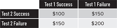
The chance that both tests succeed is 0.8 × 0.8 = 64%. The chance that one succeeds while the other fails is 0.8 × 0.2 × 2 = 32%. The chance that both fail is 0.2 × .2 = 4%. The 80th percentile for each individual event is $50 million, since there is an 80% chance that each individual test will succeed. The sum of the 80% confidence levels is $100 million. The 80th percentile for the two events considered as a portfolio is $150 million, since there is only a 64% chance that both events succeed. The portfolio 80% confidence level exceeds the sum of the 80% confidence levels for the two tests. The portfolio of these two independent events is riskier than if each one was managed completely independently of the other. This does not make sense. Two events when treated as a portfolio should not be riskier than when considered separately. Common sense would tell you that managing two projects as a portfolio should be no riskier than managing them separately. They should be less risky due to diversification benefits. However, measuring risks with percentiles can lead to the opposite conclusion. This occurs frequently whenever percentile funding is used to measure risk, and the level is below the mean. In the example, the mean test cost is 0.64 × $100 million + 0.32 × $150 million + 0.04 × $200 million = $120 million, more than the sum of the individual 80% confidence levels.

As a comparison with previous continuous distribution examples, consider a portfolio of 10 lognormal distributions, with the same means and standard deviations as in Table 5.2 but with funding of each project set to the 50th percentile. See Table 5.6.

Table 5.6 Negative Portfolio Effect When Funding Is at the 50th Percentile

Each individual project is funded at the 50th percentile. The overall funding level, which is the sum of the 50th percentiles for each project, is less than the 50th percentile. The total funding is approximately at the 36th percentile. This illustrates that when we fund individual project below the mean, things only get worse, not better, at the portfolio level. Note that the sum of the 50th percentiles for the 10 projects is $10,269, while the 50th percentile for the portfolio is $12,194. This is about 16% lower than that needed if the goal is for the overall confidence level to be at the 50th percentile.

This example is different than the others we have conducted up to this point. The prior examples all looked at a portfolio target for the confidence level. A confidence level required for each project was then determined. This is how it should be done. However, the example in Table 5.6 is how the process occurs in practice. Each individual project is funded at a set level, and then these funding levels are summed to obtain the overall funds needed for the portfolio. There is a great deal of qualitative analysis and collaborative deliberation by leadership in the budget-setting, but there is no quantitative cost risk analysis conducted at the portfolio level. No one truly knows the total confidence level.

Little upside benefits exist in funding to a percentile above the mean since there are only trivial benefits from a portfolio effect for percentile funding. However, when funding to a percentile below the mean, there is a significant downside in that the odds of overruns for the entire portfolio are worse than the odds of any individual project overrunning. See Table 5.7 for a comparison of the individual project confidence levels and the overall portfolio confidence level for 10 projects. Note that the values in Table 5.7 are based on empirical cost growth data and these values will vary in practice based on the risks for individual projects. The total mean is between the 60th and 70th percentile, so funding individual projects below that amount will result in a negative portfolio effect.

Table 5.7 Comparison of Individual Project Confidence Levels and Portfolio Confidence Level

We see from Table 5.7 that funding individual projects to the 60th percentile results in an overall confidence level for the portfolio at the 56th percentile. The effect worsens for lower levels. The gap is largest when the individual projects are funded between the 23rd and 24th percentiles (not shown in Table 5.7), in which case the overall portfolio confidence level is 13 percentage points lower. For amounts below these, the effect is not as severe and improves a little. The slight improvement is possible only because the overall portfolio confidence level is greater than zero, despite the sincere and repeated attempts of decision makers. It reminds me of a joke about a student who got a zero on a mathematics test. He asked the professor why he got a zero, and she replied that she gave him a zero only because it was impossible to give him a negative score.

Even when a project conducts a quantitative risk analysis and funds to a value that is at the mean or better, it is still likely below the true mean. This is because, as discussed in Chapter 4, risk is not assessed realistically. The 50th percentile for most risk analyses is closer to the 20% confidence level of actual risk. Underestimating risk sets up a negative portfolio effect.

A Wild Ride: The Negative Portfolio Effect for Extreme Risks

When risk has extreme variation, as exhibited by a power-law distribution such as the Pareto, a negative portfolio effect may be guaranteed regardless of the confidence level used for setting budgets for individual projects. For example, if nine projects follow a lognormal distribution and one follows a Pareto distribution with finite mean but infinite variance, budgeting each endeavor to even the 80% confidence level does not guarantee the portfolio will be funded at the 80% confidence level. See Table 5.8 for an illustration.

Table 5.8 The Negative Consequence of 50% Confidence Level Funding When Risks Are Extreme

Note that in Table 5.8, one project does not have a standard deviation listed. This is the one where risk is modeled as a Pareto distribution with finite mean but infinite standard deviation. In Table 5.8, funding projects at the 80% confidence level results in a portfolio confidence level equal to 78%, a negative portfolio effect. The wild variation and funding to a confidence level that is not in the tail of the distribution are the causes.

Low confidence levels for individual projects is bad, but low confidence levels for a portfolio is worse. If there are reserves held at the portfolio level above the project, at least some individual project overruns can be paid for with these reserves. A low confidence level for the portfolio makes a cost overrun for the entire organization more likely. Once this occurs, there is little recourse. An overrun at the portfolio level will lead to project cancellations, scope cuts, or schedule delays due to funding constraints.

SUMMARY AND RECOMMENDATIONS

You go see your financial advisor. She advises you to invest in diseased sheep. You say you think this is unwise. The sheep will likely all die, and you will lose your entire investment. She replies that would be true if you were only investing in one sheep. However, by investing in a portfolio of diseased sheep, when you aggregate the risk, it suddenly vanishes. Would you buy that argument? While it sounds silly, projects behave this way when aggregating risks to the portfolio level.

The purported notion of a portfolio effect when percentiles are used as the risk measure relies on the idea that each individual program has little risk, and that even this amount of risk dissipates once risks for multiple programs are aggregated to a portfolio level. However, as we have seen from the amounts of cost risk for historical programs, this is not a valid assumption. Many projects are breaking new ground with new technologies or using existing technologies in novel ways. This work is often challenging and has significant inherent technical risk.

We started the chapter with an example that showed a 10% savings in cost due to a portfolio effect. We showed that in practice this does not exist. We then discussed how this is handled in practice, which is that projects are typically funded at low levels and that there is no portfolio level cost risk analysis conducted. This results in a negative portfolio effect of approximately 10%. The bottom line is that all organizations, in addition to conducting risk analysis at the project level, also need to conduct risk analysis at the portfolio level. There is no shortcut provided by an imaginary portfolio effect.

The promised “free lunch” part of the portfolio effect is that projects can experience the benefits from diversification while at the same time ignoring the tails of the distribution. To benefit from diversification, the risk measure must account for the extreme risks. Percentile funding does not account for these. The existence of extreme risk must be recognized. In the next chapter, we will revisit the portfolio effect and show the issue lies largely with the way that risk is measured. With the right risk measures, a true portfolio effect will be shown to exist. This will provide the synthesis between the thesis of a portfolio effect and antithesis that it is as imaginary as a free lunch. However, the portfolio effect will still prove to be no free lunch. As we will discuss, it requires substantial amounts of risk reserves.