CHAPTER 1: Transmission

TRANSMISSION GOALS

Transmission is the conveyance of a waveform from one place to another. Transmission quality is judged by how faithfully the arriving signal tracks the original waveform. We capture the original acoustic or electronic waveform, with the intent of eventually reconstituting it into an acoustic waveform for delivery to our ears. The odds are against us. In fact there is absolutely zero probability of success. The best we can hope for is to minimize the distortion of the waveform, i.e., damage control. This is the primary goal of all efforts described in this book. This may sound dispiriting, but it is best to begin with a realistic assessment of the possibilities. Our ultimate goal is one that can be approached, but never reached. There will be large numbers of decisions ahead, and they will hinge primarily on which direction provides the least damage to the waveform. There are precious few avenues that will provide none, and often the decision will be a very fine line.

Our main study of the transmission path will look at three modes of transmission: line level electronic, speaker level electronic, and acoustic. If any link in the transmission chain fails, our mission fails. By far the most vulnerable link in the chain is the final acoustical journey from the speaker to the listener. This path is fraught with powerful adversaries in the form of copies of our original signal (namely reflections and arrivals from the other speakers in our system), which will distort our waveform unless they are exact copies and exactly in time. We will begin with a discussion of the properties of transmission that are common to all parts of the signal path (Fig. 1.1).

AUDIO TRANSMISSION DEFINED

An audio signal undergoes constant change, with the motion of molecules and electrons transferring energy away from a vibrating source. When the audio signal stops changing, it ceases to exist as audio. As audio signals propagate outwards, the molecules and electrons are displaced forward and back but never actually go anywhere, always returning to their

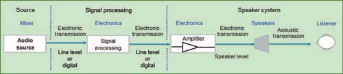
FIGURE 1.1
Transmission flow from the signal source to the listener.

point of origin. The parameter that describes the extent of the change is the amplitude, also referred to as magnitude. A single round trip from origin and back is a cycle. The round trip takes time. That length of time is the period and is given in seconds, or for practical reasons in milliseconds (ms). The reciprocal of the period is frequency, the number of cycles completed per second, given in hertz (Hz). The round trip is continuous with no designated beginning or end. The trip can begin anywhere on the cycle and is completed upon our return to the same position. The radial nature of the round trip requires us to find a means of expressing our location around the circle. This parameter is termed the phase of the signal. The values are expressed in degrees, ranging from 0° (point of origin) to 360° (a complete round trip). The half-cycle point in the phase journey, 180°, will be of particular interest to us as we move forward.

All transmission requires a medium, i.e., the entity through which the audio signal passes from point to point, made of molecules or electrons. In our case, the primary media are wire (electronic) and air (acoustic), but there are interim media as well such as magnetic and mechanical. The process of transferring the audio energy between media is known as transduction. The physical distance required to complete a cycle in a particular medium is the wavelength and is expressed in some form of length, typically meters or feet. The size of the wavelength for a given frequency is proportional to the transmission speed of our medium.

The physical nature of the waveform's amplitude component is medium-dependent. In our acoustical case, the medium is air and the vibrations are expressed as a change in pressure. The half of the cycle with higher than the ambient pressure is termed pressurization, while the low-pressure side is termed rarefaction. A loudspeaker's forward motion into the air creates pressurization and its rearward movement creates rarefaction.

The movements of speaker cones do not push air across the room in the manner of a fan. If a room is hot, it is unlikely that loud music will cool things down. Instead air is moved forward and then it is pulled back to its original position. The transmission passes through the medium, which is an important distinction. Multiple transmissions can pass through the medium simultaneously even from different directions.

Electrical pressure change is expressed as positive and negative voltage. This movement is also termed alternating current (AC) since it fluctuates above and below the ambient voltage. A voltage that maintains a constant value over time is termed direct current (DC).

Our design and optimization strategies require a thorough understanding of the relationships between frequency, period, and wavelength.

Time and frequency

Let's start with a simple tone, a sine wave, and the relationship of frequency (F) and period (T):

T = 1/F  and  F = 1/T

where T is the time period of a single cycle in seconds and F is the number of cycles per second (Hz).

To illustrate this point, we will use a convenient frequency and delay for clarity: 1000 Hz (or 1 kHz) and 1/1000th of a second (or 1 ms).

If we know the frequency, we can solve for time. If we know time, we can solve for frequency. Therefore

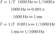
For most of this text, we abbreviate the time period to the term “time” to connote the cycle duration of a particular frequency (Fig. 1.2).

Frequency is the best-known parameter since it is closely related to the musical term “pitch.” Most audio engineers relate first in musical terms since few of us got into this business because of a lifelong fascination with acoustical physics. We must go beyond frequency/pitch, however, since our job is to “tune” the sound system, not tune the musical instruments. Optimization strategies require an ever-present three-way link between frequency, period, and wavelength. The frequency 1 kHz exists only with its reciprocal sister 1 ms. This is not medium-dependent, nor temperature-dependent, nor waiting upon a standards committee ruling. This is one of audio's few undisputed absolutes. If the audio is traveling in a wire, those two parameters will be largely sufficient for our discussions. Once in the air, we will need to add the third dimension: wavelength. A 1 kHz signal only exists in air as a wavelength about as long as the distance from our elbow to our fist. All behaviors at 1 kHz are governed by the physical reality of the signal's time period and its wavelength. The first rule of optimization is to never think of an acoustical signal without consideration of all three parameters.

Wavelength

Wavelength is proportional to the medium's unique transmission speed. A given frequency will have a different wavelength in its electronic form (over 500,000 × larger) than its

FIGURE 1.2
Amplitude vs. time converted to amplitude vs. frequency.

TABLE 1.1 Speed of sound reference

Plain language	Imperial/American measurement	Metric measurement
Speed of sound in air at 0°	1052 ft/s	331.4 m/s
+Adjustment for ambient air temperature	+(1.1 × T) Temperature T in °F	+(0.607 × T) Temperature T in °C
= Speed of sound at ambient air temperature	= c feet/second	= c meters/second

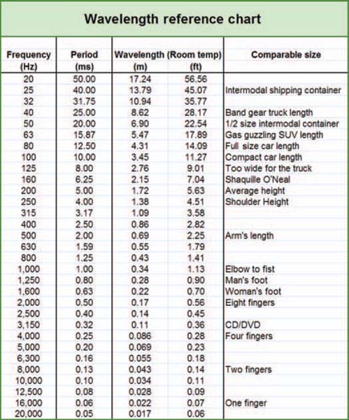
FIGURE 1.3
Chart of frequency, period, and wavelength (at room temperature) for standard one-third octave frequencies.

acoustic version. If the medium is changed, its transmission speed and all the wavelengths change with it.

The wavelength formula is

L = c/F

where L is the wavelength in meters, c is the transmission speed of the medium, and F is the frequency (Hz).

Transmission speed through air is among the slowest. Water is a far superior medium in terms of speed and high-frequency (HF) response; however, the hazards of electrocution and drowning make this an unpopular sound reinforcement medium (synchronized swimming aside). We will stick with air.

The formulas for the speed of sound in air are as shown in Table 1.1.

For example, at 22°C:

c = (331.4 + 0.607 × 22)m/s

c = 344.75 m/s

The audible frequency range given in most books is 20 Hz to 20 kHz. Few loudspeakers are able to reproduce the 20 Hz or 20 kHz extremes at a power level sufficient to play a significant role. It is more useful to limit the discussion to those frequencies we are likely to encounter in the wild: 31 Hz (the low B note on a five-string bass) up to 18 kHz. The wavelengths within this band fall into a size range of between the width of a finger and a standard intermodal shipping container. The largest wavelengths are about 600 times larger than the smallest (Figs 1.3–1.5).

Why it is that we should be concerned about wavelength? After all, there are no acoustical analyzers that show this on their display. There are no signal-processing devices that depend on this for adjustment. In practice, there are some applications where we can be blissfully ignorant of wavelength, for example: when we use a single loudspeaker in a reflection-free environment. For all other applications, wavelength is not simply relevant: it is decisive. Wavelength is the critical parameter in acoustic summation. The combination of signals at a given frequency is governed by the number of wavelengths that separate them. There is a lot at stake here, as evidenced by the fact that Chapter 2 is dedicated exclusively to this subject: summation. Combinations of wavelengths can range from maximum addition to maximum cancellation. Since we are planning on doing lots of combining, we had best become conscious of wavelength.

TEMPERATURE EFFECTS

As we saw previously, the speed of sound in air is slightly temperature-dependent. As the ambient temperature rises, sound speed increases and therefore the wavelengths expand. This behavior may slightly affect the response of our systems over the duration of a performance, since the temperature is subject to change even in the most controlled environments. However, although it is often given substantial attention, this is rarely a major factor in the big picture. A poorly designed system is not likely to find itself rescued by weather changes. Nor is it practical to provide ongoing environmental analysis over the widespread areas of an audience to compensate for drafts in the room. For our discussion, unless otherwise specified, we will consider the speed of sound to be fixed approximately at room temperature.

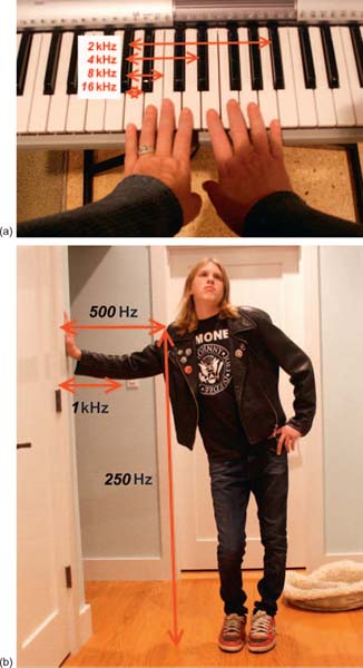
FIGURE 1.4
Handy reference for short wavelengths.

The relationship between temperature and sound speed can be approximated as follows: a 1% change in the speed of sound occurs with either a 5°C or 10°F change in temperature.

Waveform

There is no limit to the complexity of the audio signal. Waves at multiple frequencies may be simultaneously combined to make a new and unique signal that is a mixture of the contributing signals. This composite signal is the waveform, containing an unlimited combination of audio frequencies with variable amplitude and phase relationships. The waveform's complex shape depends upon the components that make it up and varies constantly as they do. A key parameter is how the frequency content of the contributing signals affects the combined waveform (Figs 1.6–1.8). When signals at different frequencies are added, the combined waveform will carry the shape of both components independently. The higher frequency is added to the shape of the lower-frequency waveform. The phase of the individual frequencies will affect the overall shape but the different frequencies maintain their separate identities. These signals can be separated later by a filter (as in your ear) and heard as separate sounds. When two signals of the same frequency are combined, a new and unique signal is created that cannot be filtered apart. In this case, the phase relationship has a decisive effect upon the nature of the combined waveform.

Analog waveform types include electronic, magnetic, mechanical, optical, and acoustical. Digital audio signals are typically electronic, magnetic, or optical, but the mechanics of the digital data transfer are not critical here. It could be punch cards as long as we can move them fast enough to read the data. Each medium tracks the waveform in different forms of energy, suitable for the particulars of that transmission mode, complete with its own vulnerabilities and limitations. Digital audio is most easily understood when viewed as a mathematical rendering of the waveform. For these discussions, this is no different from analog, which in any of its resident energy forms can be quantified mathematically.

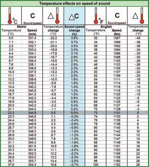
FIGURE 1.5
Chart of speed of sound, period, and wavelength at different temperatures.

The audio signal can be visualized in three different forms as shown in Fig. 1.9. A single cycle is broken into four quadrants of 90° each. This motion form illustrates the movement of the signal from a point of rest to maximum amplitude in both directions and finally returning to the origin. This is representative of the particle motion in air when energized by a sound source such as a speaker. It also helps illustrate the point that the motion is back and forth rather than going outward from the speaker. A speaker should not be confused with a blower. The maximum displacement is found at the 90° and 270° points in the cycle. As the amplitude

FIGURE 1.6
Reference chart of some of the common terms used to describe and quantify an audio waveform.

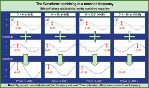
FIGURE 1.7
Combination of waveforms of the same frequency at the same level with different phase relationships: (a) 0° relative phase combines to +6 dB amplitude, (b) 90° relative phase combines to +3 dB amplitude, (c) 120° relative phase combines to +0 dB, (d) 180° relative phase cancels.

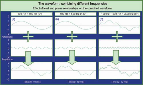
FIGURE 1.8
Combination of waveforms of different frequencies with different levels and phase relationships. (a) Second frequency is 5 × higher and 12 dB down in level from the first. Phase relationship is 0°. Note that both frequencies can be seen in the combined waveform. (b) Same as (a) but with relative phase relationship at 180°. Note that there is no cancellation in the combined waveform. The orientation of the HF trace has moved but the LF orientation is unchanged. (c) Combined waveform of (a) with third frequency added. The third frequency is 25 × the lowest frequency and 18 dB down in level. The phase relationship is matched for all frequencies. Note that all three frequencies can be distinguished in the waveform.

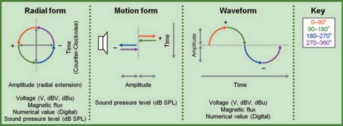
FIGURE 1.9
Three representations of the audio waveform.

increases, the displacement from the equilibrium point becomes larger. As the frequency rises, the time elapsed to complete the cycle decreases.

The radial form represents the signal as spinning in a circle. The waveform origin point corresponds to the starting point phase value, which could be any point on the circle. A cycle is completed when we have returned to the phase value of the point of origin. This representation shows the role that phase will play. The difference in relative positions on this radial chart of any two sound sources will determine how the systems will react when combined.

The sinusoidal waveform representation is the most familiar to audio engineers and can be seen on any oscilloscope. The amplitude value is tracked over time and traces the waveform in the order in which the signal passes through. This is representative of the motion over time of transducers and changing electrical values of voltage over time. Analog-to-digital (A/D) converters capture this waveform and create a mathematical valuation of the amplitude vs. time waveform.

TRANSMISSION QUANTIFIED

Decibels

Transmission amplitudes, also known as levels, are most commonly expressed in decibels (dB), a unit that describes a ratio between two measures. The decibel is a logarithmic scaling system used to describe ratios with a very large range of values. Using the decibel has the added benefit of closely matching our perception of sound levels, which is generally logarithmic. There are various dB scales that apply to transmission. Because decibels are based on ratios, they are always a relative scale. The question is: relative to what? In some cases, we compare to a fixed standard. Because audio is in constant change, it is also useful to have a purely relative scale that compares two unknown signals. An example of the latter type is the ratio of output to input level. This ratio, the gain of the device, can be quantified even though a drive signal such as music is constantly changing. If the same voltage appears at the output and input, the ratio is 1, also known as unity gain, or 0 dB. If the voltage at the output is greater, the gain value exceeds 1, and expressed in dB, is positive. If the input is greater, the gain ratio is less than 1 and expressed in dB is a negative number, signifying a net loss. The actual value at the input or output is unimportant. It is the change in level between them that is reflected by the dB gain value.

There are two types of log formulas applicable in audio:

 

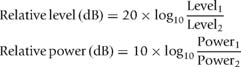
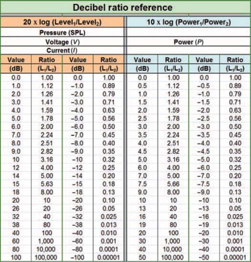
FIGURE 1.10
The ratio of output to input can be converted to dB with this easy reference chart. To compare a given level to a standard one, Level1 is the given level and Level2 is the standard. To derive the gain of a device, Level1 is the output level and Level2 is the input level. Likewise the power gain can be found in the same manner by substituting the power parameters.

Power-related equations use the 10 log version, while pressure- (SPL) and voltage-related equations use the 20 log version. It is important that the proper formula be used since a doubling of voltage is a change of 6 dB while a doubling of power is a change of 3 dB. For the most part, we will be using the 20 log version since acoustic pressure (dB SPL) and voltage are the primary drivers of our decision-making. Figure 1.10 provides a reference chart to relate the ratios of values to their decibel equivalents.

Here is a handy tip for Microsoft Excel users. Figure 1.11 shows the formula format for letting Excel do the log calculations for us.

THE ELECTRONIC DECIBEL: dBV AND dBu

Electronic transmission utilizes the decibel scale to characterize the voltage levels. The decibel scale is preferred by operators over the linear scale for its relative ease of expression. Expressed linearly, we would find ourselves referring to the signal in microvolts, millivolts, and volts with various sets of number values and ranges. Such scaling makes it difficult to track a variable signal such as music. If we wanted to double the signal level, we would have to first know the voltage of the original signal and then compute its doubling. With dynamically changing signals such as music, the level at any moment is in flux, making such calculations impractical. The decibel scale provides a relative change value independent of the absolute value. Hence the desire to double the level can be achieved by a change of 6 dB, regardless of the original value. We can also relate the decibel to a fixed standard, which we designate as “0 dB.” Levels are indicated by their relative value above (+dB) or below (−dB) this standard. This would be simplest, of course, if there were a single standard, but tradition in our industry is to pick several. dBV and dBu are the most common currently. These are referenced to different values of 1.0 and 0.775 V (1mW across a 600Ω load) respectively. The difference between these is a fixed amount of 2.21 dB. Note: For ease of use, we will use dBV as the standard in this text. Those who prefer the dBu standard should apply +2.21 dB to the given dBV values.

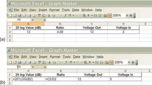
FIGURE 1.11
Microsoft Excel log formula reference.

The voltage-related dB scales serve the important purpose of guidance toward the optimal operating range of the electronic devices. The upper and lower limits of an electronic device are absolute, not relative values. The noise floor has a steady average level and the clip point is a fixed value. These are expressed in dBV. The absolute level of our signal will need to pass between these two limits in order to prevent excess noise or distortion. The area enclosed by these limits is the linear operating area of the electronic device. Our designs will need to ensure that the operating levels of electronic devices are appropriately scaled for the signal levels passing through.

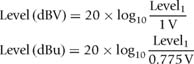
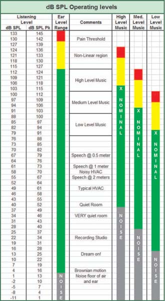
Once we have captured the audio waveform in its electronic form, it will be passed through the system as a voltage level with negligible current and therefore minimal power dissipation. Low-impedance output sections, coupled with high-impedance inputs, give us the luxury of not considering the power levels until we have reached the amplifier output terminals. Power amplifiers can then be seen as voltage-driven input devices with power stage outputs to drive the speakers. The amplifier gives a huge current boost and additional voltage capability as well. Figure 1.12 provides a reference chart showing the standard operating voltage levels for all stages of the system signal flow. The goal is to transmit the signal through the system in the linear operating voltage range of all of the devices, without falling into the noise floor at the bottom.

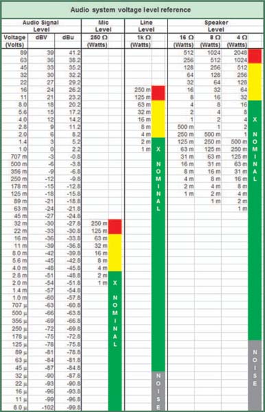
FIGURE 1.12
Reference chart for the typical operational voltage and wattage levels at various stages of the audio transmission. All voltages are RMS.

There is still another set of letter appendices that can be added on to the dB voltage formulas. These designate whether the voltage measured is a shortterm peak or the average value. AC signals are more complex to characterize than DC signals. DC signals are a given number of volts above or below the reference common. AC signals, by nature, go both up and down. If an average were taken over time, we would conclude that the positive and negative travels of the AC signal average out to 0 V. Placing our fingers across the AC mains will quickly alert us to the fact that averaging out to 0 V over time does not mean there is zero energy there. Kids, don't try this at home.

The AC waveform rises to a maximum, returns to zero, falls to a minimum, and then returns again to zero. The voltage between the peak and the zero point, either positive or negative, is the peak voltage (V_pk). The voltage between the positive and negative peaks is the peak-to-peak voltage (V_p−p) and is naturally double that of the peak value. The equivalent AC voltage to that found in a DC circuit is expressed as the root-mean-square (RMS) voltage (V_RMS). The relationship between the peak and RMS values varies depending on the shape of the AC waveform. The RMS value is 70.7% of the peak value.

All of these factors translate over to the voltage-related dB formulas and are found as dBV_pk, dBV_p−p, and dBV_RMS respectively. The 70.7% difference between peak and RMS is equivalent to 3 dB.

Crest factor

The term to describe the variable peak-to-RMS ratio found in different program materials is the crest factor (Fig. 1.13). The waveform with the lowest possible crest factor (3 dB) is a sine wave, which has a peak/RMS value of 1.414 (or RMS/peak value of 0.707). The presence of multiple frequencies creates momentary confluences of signals that can sum together into a peak that is higher than any of the individual parts. This is known as a transient peak. Most audio signals are transient by nature since we can't dance to sine waves. A strong transient, like a pulse, is one that has a very high peak value and a minimal RMS value. Transient peaks are the opposite extreme of peak-to-RMS ratio from the sine wave. Theoretically, there is no limit to the maximum, but our audio system will require more dynamic range as crest factor increases. The typical crest factor for musical signals is 12 dB. Since our system will be transmitting transients and continuous signals, we must ensure that the system has sufficient dynamic range to allow the transient peaks to stay within the linear operating range. The presence of additional dynamic range above the ability to pass a simple sine wave is known as headroom, with 12 dB being a common target range.

ACOUSTIC DECIBEL: dB SPL

The favored expression for acoustic transmission is dB SPL (sound pressure level). This is the quantity of measure for the pressure changes above and below the ambient air pressure. The standard is the threshold of the average person's hearing (0 dB SPL). The linear unit of expression is one of pressure, dynes/square centimeter, with 0 dB SPL being

FIGURE 1.13
Crest factor, RMS, peak, and peak-to-peak values. (a) A sine wave has the lowest crest factor of 3 dB. (b) An example complex waveform with transients with a 12 dB crest factor.

a value of 0.0002 dynes/cm² (1 μbar). This lower limit approaches the noise level of the air medium, i.e., the level where the molecular motion creates its own random noise. It is comforting to know we aren't missing out on anything. At the other end of the scale is the threshold of pain in our hearing system. The values for this are somewhat inconsistent but range from 120 to 130 dB SPL, with more modern texts citing the higher numbers (Fig. 1.14). In any case, this number represents the pain threshold, and with that comes the obvious hazards of potential hearing damage:

where P is the RMS pressure in microbars (dynes/ square centimeter).

Excuse me: did you say microbars and dynes per square centimeter?

FIGURE 1.14
Typical operational level over the dynamic range of the ear.

These air pressure measurement terms are unfamiliar to most audio engineers, along with the alternate and equally obscure term of 20 μPa. For most audio engineers, the comprehension of dB SPL is relative to their own perspective: an experiential correlation to what we hear with what we have read over the years on SPL meters. The actual verification of 0 dB SPL is left to the Bureau of Standards and the people at the laboratories. Few of us have met a dyne, a microbar, or a micropascal at the venue or ever will. Even fewer are in a position to argue with someone's SPL meter as to whether it is calibrated correctly, unless we have an SPL meter and a calibrator of our own to make the case. Then we can argue over whose calibrator is accurate and eventually someone must yield or we will have to take a trip to the Bureau of Standards. This is one place where, in our practical world, we will have to take a leap of faith and trust the manufacturers of our measurement microphones. For our part, we will be mindful of even small discrepancies between different measurement instruments, microphones, etc., but we will not be in a good position to question the absolute dB SPL values to the same extent.

The 130 dB difference between the threshold of audibility and the onset of pain can be seen as the dynamic range of our aural system. Our full range will rarely be utilized, since there are no desirable listening spaces with such a low noise floor. In addition, the ear system is generating substantial harmonic distortion before the pain threshold which degrades the sonic experience (for some) before actual pain is sensed. In practical terms, we will need to find a linear operating range, as we did for the electronic transmission. This range runs from the ambient noise floor to the point where our hearing becomes so distorted that the experience is unpleasant. Our sound system will need to have a noise floor below the room and sufficient continuous power and headroom to reach the required maximum level.

dB SPL subunits

dB SPL has average and peak level in a manner similar to the voltage units. The SPL values differ, however, in that there may be a time constant involved in the calculation.

■ dB SPL peak: The highest level reached over a measured period is the peak (dB SPL_pk).

■ dB SPL continuous (fast): This is the average SPL over a time integration of 250 ms. The integration time is used in order to mimic our hearing system's perception of SPL. Our hearing system does not perceive SPL on an instantaneous level but rather over a period of approximately 100 ms. The fast integration is sufficiently long enough to give an SPL reading that corresponds to that perception.

■ dB SPL continuous (slow): This is the average SPL over a time integration of 1 s. The slower time constant mimics the perception of exposure to extended durations of sound.

■ dB SPL LE (long term): This is the average SPL over a very long period of time, typically minutes. This setting is typically used to monitor levels for outdoor concert venues that have neighbors complaining about the noise. An excessive LE reading can cost the band a lot of money.

dB SPL can be limited to a specific band of frequencies. If a bandwidth is not specified, the full range of 20 Hz–20 kHz is assumed. It is important to understand that a reading of 120 dB SPL on a sound level meter does not mean that a speaker is generating 120 dB SPL at all frequencies. The 120 dB value is the integration of all frequencies (unless otherwise specified) and no conclusion can be made regarding the behavior over the range of speaker response. The only case where the dB SPL can be computed regarding a particular frequency is when only that frequency is sent into the system. dB SPL can also be determined for a limited range of frequencies, a practice known as banded SPL measurements. The frequency range of the excitation signal is limited, commonly in octave or one-third octave bands, and the SPL over that band can be determined. The maximum SPL for a device over a given frequency band is attained in this way. It is worth noting that the same data cannot be attained by simply band-limiting on the analysis side. If a fullrange signal is applied to a device, its energy will be spread over the full band. Bandlimited measurements will show lower maximum levels for a given band if the device is simultaneously charged with reproducing frequencies outside of the measured band.

THE UNITLESS DECIBEL

The unitless decibel scale is available for comparison of like values. Everything expressed in the unitless scale is purely relative. This can be applied to electronic or acoustic transmission. A device with an input level of +20 dBV and an output level of +10 dBV has a gain of +10 dB. Notice that no letter is appended to the dB term here, signifying a ratio of like quantities. Two seats in an auditorium that receive 94 and 91 dB SPL readings respectively are offset in level by 3 dB. This is not expressed as 3 dB SPL, a level just above our hearing threshold. If the levels were to rise to 98 and 95 respectively, the level offset remains at 3 dB.

The unitless dB scale will be by far the most common decibel expression in this book. The principal concern of this text is relative level, rather than absolute levels. Simply put, absolute levels are primarily an operational issue, inside the scope of mix engineering, whereas relative levels are primarily a design and optimization issue, under our control. The quality of our work will be based on how closely the final received signal resembles the original. Since the transmitted signal will be constantly changing, we can only view our progress in relative terms.

Power

Electrical energy is a combination of two measurable quantities: voltage and current. The electrical power in a DC circuit is expressed as:

P = EI

where P is the power in watts, E is the voltage in volts, and I is the current in amperes.

Voltage corresponds to the electrical pressure while current corresponds to the rate of electron flow. A simplified analogy comes from a garden hose. With the garden hose running open, the pressure is low and the flow is a wide cylinder of water. Placing our thumb on the hose will greatly increase the pressure and reduce the width of the flow by a proportional amount. The former case is low voltage and high current, while the latter is the reverse.

The power is the product of these two factors; 100 watts (W) of electrical power could be the result of 100 volts (V) at 1 amperes (A), 10 V at 10 A, 1 V at 100 A, etc. The power could be used to run one heater at 100 W, or 100 heaters at 1 W each. The heat generated, and the electrical bill, is the same either way. Both voltage and current must be present for power to flow. Voltage with no current is potential for power, but none is transferred until current flows.

A third factor plays a decisive role in how the voltage and current are proportioned: resistance. Electrical resistance limits the amount of current flowing through a circuit and thereby affects the power transferred. Provided that the voltage remains constant, the power dissipation will be reduced as the resistance stems the flow of current. This power reduction can be compensated by an increase in voltage proportional to the reduced current. Returning to the garden hose analogy, it is the thumb that acts as a variable resistance to the circuit, a physical feeling that is quite apparent as we attempt to keep our thumb in place. This resistance reapportions the hose power toward less current flow and higher pressure. This has very important effects upon how the energy can be put to use. If we plan on taking a drink out of the end of the hose, it would be wise to carefully consider the position of our thumb.

The electrical power in a DC circuit is expressed as:

P = IE

P = I²R

P = E²/R

where P is the power in watts, E is the voltage in volts, I is the current in amperes, and R is the resistance in ohms.

These DC formulas are applicable to the purely resistive components of the currentlimiting forces in the electrical circuit. In the case of our audio waveform, which is by definition an AC signal, the measure of resistive force differs over frequency. The complex term for resistance with a frequency component is impedance. The impedance of a circuit at a given frequency is the combination of the DC resistance and the reactance. The reactance is the value for variable resistance over frequency and comes in two forms: capacitive and inductive. The impedance for a given circuit is a combination of the three resistive values: DC resistance, capacitive reactance, and inductive reactance. These factors alter the frequency response in all AC circuits; the question is only a matter of degree of effect. For our discussion here, we will not go into the internal circuit components but rather limit the discussion of impedance and reactance to the interconnection of audio devices. All active audio devices present an input and output impedance and these must be configured properly for optimal transmission. The interconnecting cables also present variable impedance over frequency and this will be discussed.

Frequency response

If a device transmits differently at one frequency than another, it has a frequency response. A device with no differences over frequency, also known as a “flat” frequency response, is actually the absence of a frequency response. In our practical world, this is impossible, since all audio devices, even oxygen-free hypoallergenic speaker cable, change their response over frequency. The question is the extent of detectable change within the frequency and dynamic range of our hearing system. Frequency response is a host of measurable values but we will focus our discussion in this section on two representations: amplitude vs. frequency and phase vs. frequency. No audio device can reach an infinitely low frequency (we would have to go all the way back to the Big Bang to measure the lowest frequency) and none can reach an infinitely high frequency. Fortunately this is not required. The optimal range is some amount beyond that of the human hearing system. (The exact extent is subject to ongoing debate.) It is generally accepted that HF extension beyond the human hearing limits is preferable to those systems that limit their response to exactly 20 Hz to 20 kHz. This is generally attributed to the reduced phase shift of the in-band material, which leaves the upper harmonic series intact. Anyone familiar with the first generations of digital audio devices will remember the unnatural quality of the band-limited response of those systems. The debate over 96 kHz, 192 kHz, and higher sampling rates for digital audio will be reserved for those with ears of gold.

AMPLITUDE VS. FREQUENCY

Amplitude vs. frequency (for brevity, we will call this the amplitude response) is a measure of the level deviation over frequency. A device is specified as having an operational frequency range and a degree of variation within that range. The frequency range is generally given as the −3 dB points in electronic devices, while −6 and −10 dB figures are most often used for speakers. The quality of the amplitude response is determined by its degree of variance over the transmission range, with minimum variance corresponding to the maximum quality. The speakers shown in Fig. 1.15 have an amplitude response that is ±4 dB over their operating ranges. The operating ranges (between −6 dB points) differ in the low frequency (40 and 70 Hz) and high frequency (18 and 20 kHz).

PHASE VS. FREQUENCY

Phase vs. frequency (for brevity, we will call this the phase response) is a measure of the time deviation over frequency. A device is specified as having a degree of variation within the operational range governed by the amplitude response. The quality of the phase response is determined by its degree of variance over the transmission range, with minimum variance again corresponding to the maximum quality. The phase responses of the two speakers we compared previously in Fig. 1.15 are shown as an example.

The phase response over frequency is, to a large extent, a derivative of amplitude response over frequency. Leaving the rare exception aside for the moment, we can say that a flat phase response requires a flat amplitude response. Deviations in the amplitude response over frequency (peak and dip filters, high- and low-pass filters, for example) will cause predictable deviations in phase. Changes in amplitude that are independent of frequency are also independent of phase; i.e., an overall level change does not affect phase.

The exception cited above refers to filter circuits that delay a selective range of frequencies, thereby creating phase deviations unrelated to changes in amplitude. This creates interesting possibilities for phase compensation in acoustical systems with physical displacements between drivers. The final twist is the possibility of filters that change

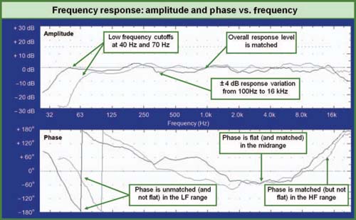
FIGURE 1.15
Relative amplitude and relative phase responses of two loudspeakers. The two systems are matched in both level and phase over most of the frequency range, but become unmatched in both parameters in the LF range.

amplitude without changing phase. The quest for such circuits is like a search for the Holy Grail in our audio industry. We will revisit this quest later in Chapter 10. Phase will be covered from multiple perspectives as we move onward. For now, we will simply introduce the concept.

Phase response always merits a second-place finish in importance to amplitude response for the following reason: if the amplitude value is zero, there is no level, and the phase response is rendered academic. In all other cases, however, the response of phase over frequency will need to be known.

There has been plenty of debate in the past as to whether we can discern the phase response over frequency of a signal. The notion has been advanced that we cannot hear phase directly and therefore a speaker with extensive phase shift over frequency was equivalent to one that exhibited flat phase. This line of reasoning is absurd and has few defenders left. Simply put, a device with flat phase response sends all frequencies out in the temporal sequence as they went in. A device with nonlinear phase selectively delays some frequencies more than others. These discussions are typically focused on the performance of loudspeakers, which must overcome tremendous challenges in order to maintain a reasonably flat phase response for even half of their frequency range. Consider the following question: all other factors being equal, would a loudspeaker with flat phase over a six-octave range sound better than one that is different for every octave? The answer should be self-evident unless we subscribe to the belief that loudspeakers create music instead of recreating it. If this is the case, then I invite you to consider how you would feel about your console, cabling or amplifiers contributing the kind of wholesale phase shift that is justified as a musical contribution by the speaker.

A central premise of this book is that the loudspeaker is not given any exception for musicality. Its job is as dry as the wire that feeds it an input signal: track the waveform. There will be no discussion here as to which forms of coloration in the phase or amplitude response sound “better” than another.

Let's apply this principle to a musical event: a piano key is struck and the transient pressure peak contains a huge range of frequency components, arranged in the distinct order that our ear recognizes as a piano note. To selectively delay some of the portions of that transient peak rearranges the sequences into a waveform that is very definitely not the original and is less recognizable as a piano note. As more phase shift is added, the transient becomes increasingly stretched over time. The sense of impact from a hammer striking a string will be lost.

While linear phase over frequency is important, it is minor compared to the most critical phase parameter: its role in summation. This subject will be the detailed in Chapter 2.

Polarity

The polarity of a signal springs from its orientation to the origin point of the waveform. All waveforms begin at the “ambient” state in the medium and proceed back and forth from there. The same waveform shape can be created in opposite directions, one going back and forth while the other goes forth and back. There is plenty of debate as to whether we can discern the absolute polarity of a signal. A piano key is struck and the pressure peak arrives first as a positive pressure followed by a negative. If this is reproduced by an otherwise perfect speaker but reversed in polarity would we hear the difference? The debate continues.

 

In our case, the critical parameter regarding polarity is ensuring that no reversals occur in parts of the transmission chain that will be combined either electrically or acoustically. Combining out of polarity signals will result in cancellation, a negative effect of which there is little debate.

Latency

Transmission takes time. Every stage in the path from the source to the listener takes some amount of time to pass the signal along. This type of delay, known as latency, occurs equally at all frequencies, and is measured in (hopefully) ms. The most obvious form of latency is the “flight time” of sound propagating through the air. The electronic path is also fraught with latency issues, and this will be of increasing importance in the future. In purely analog electronic transmission, the latency is so small as to be practically negligible. For digital systems, the latency can never be ignored. Even digital system latencies as low as 2 ms can lead to disastrous results if the signal is joined with others at comparable levels that have analog paths (0 ms) or alternate network paths (unknown number of ms). For networked digital audio systems, latency can be a wide-open variable. In such systems, it is possible to have a single input sent to multiple outputs each with different latency delays, even though they are all set to “0 ms” on the user interface.

ANALOG AUDIO TRANSMISSION

We have discussed the frequency, period, wavelength, and the audio waveform above. It is now time to focus on the transmission of the waveform through the electronic and acoustic media. We will begin with the far less challenging field of electronic transmission.

Electronic audio signals are variations in voltage, current, or electromagnetic energy. These variations will finally be transformed into mechanical energy at the speaker. The principal task of the electronic transmission path is to deliver the original signal from the console to the mechanical/acoustic domain. This does not mean that the signal should enter the acoustic domain as an exact copy of the original. In most cases, it will be preferable to modify the electrical signal in anticipation of the effects that will occur in the acoustic domain. Our goal is a faithful copy at the final destination: the listening position. To achieve this, we will need to precompensate for the changes caused by interactions in the space. The electronic signal may be processed to compensate for acoustical interaction, split apart to send the sound to multi-way speakers and then acoustically recombined in the space.

The analog audio in our transmission path runs at two standard operational levels: line and speaker. Each of these categories contains both active and passive devices. Active line level devices include the console, signal processing such as delays, equalization, level controls, and frequency dividers and the inputs of power amplifiers. Passive devices include the cables, patchbays, and terminal panels that connect the active devices together. Active devices are categorized by their maximum voltage and current capability into three types: mic, line, and speaker level. Mic and line both operate with high-impedancebalanced inputs (receivers) and low-impedance-balanced outputs (sources). Input impedances of 5–100 kΩ and output drives of 32–200Ω are typical. Mic level devices overload at a lower voltage than line level, which should be capable of approximately 10 V (+20 dBV) at the inputs and outputs. Since our discussion is focused on the transmission side of the sound system, we will be dealing almost exclusively with line level signals. Power amplifiers have a high-impedance line level input and an extremely low-impedance speaker level output. Speaker level can range to over 100 V and is potentially hazardous to both people and test equipment alike.

Line level devices

Each active device has its own dedicated functionality, but they all share common aspects as well. All of these devices have input and output voltage limits, residual noise floor, distortion, and frequency–response effects such as amplitude and phase variations. Looking deeper, we find that each device has latency, low-frequency (LF) limits approaching DC, and HF limits approaching light. In analog devices, these factors can be managed such that their effects are practically negligible—but this cannot be assumed. The actual values for all of the above factors can be measured and compared to the manufacturer's specification and to the requirements of our project.

The typical electronic device will have three stages: input, processing, and output, as shown in Fig. 1.16. The nature of the processing stage depends upon the function of the device. It could be an equalizer, delay, frequency divider, or any audio device. It could be analog or digital in the processing section but the input and output stages are analog. Professional line level electronic devices utilize a fairly standard input and output configuration: the balanced line. Balanced lines provide a substantial degree of immunity from noise induced on the line (electromagnetic interference) and grounding problems (hum) by virtue of the advantages of the differential input (discussed later in this chapter). The standard configuration is a voltage source system predicated on lowimpedance outputs driving high-impedance inputs. This relationship allows the interconnection to be relatively immune to distance and number of devices.

Now let's look at some of the particular types of devices in common use in our systems. The list that follows is by no means comprehensive. The descriptions for this limited list are mostly generic and established features and applications of these devices. There are simply too many devices to describe. The description of and advocacy for (or against) the specific features and benefits of any particular make and model will be left to the manufacturers. Therefore, consider the insertion of text such as “in most cases,” “typically but not always,” “usually,” “in every device I ever used in the last 20 years,” or “except for the model X” as applicable to any of the descriptions that would otherwise seem to exclude a particular product.

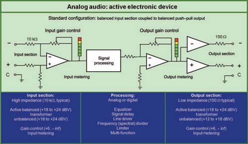
FIGURE 1.16
Typical analog electronic device flow chart.

AUDIO SOURCES

The device transmitting our original transmitted signal must be capable of delivering the signal in the working condition. The most common delivery devices are the mix console outputs. The console outputs should meet the above criteria in order for us to have an input signal worth transmitting.

SIGNAL PROCESSING

The signal-processing devices will be used during the optimization procedures. The processing may be in a single chassis, or separated, but will need the capability to perform the basic functions of calibration: level setting, delay setting, and equalization. Since these will be covered separately, we will consider the functions of the signal processor as the combination of individual units.

LEVEL-SETTING DEVICES

Level-setting devices adjust the voltage gain through the system and optimize the level for maximum dynamic range and minimum level variance by adjusting subsystem relative levels. The level-setting device ensures that the transition from the console to the power amplifier stage is maintained within the linear operating range. The resolution of a levelsetting device for system optimization should be at least 0.5 dB.

DELAY LINES

Just as level controls adjust the relative levels, the delay lines control relative phase. They have the job of time management. They aid the summation process by phase aligning acoustical crossovers for maximum coupling and minimum variance. Most delay lines have a resolution of 0.02 ms or less, which is sufficient. The minimum latency value is preferred. Most delay line user interfaces give false readings as to the amount of delay they are actually adding to the signal. The indicator on the device gives the impossible default setting of 0 ms, which is accurate only as an indication of the amount of delay added to the latency base value. An accurate unit of expression for this would be 0 ms(R); i.e., relative. If every device in the system is the same model and they are not routing signals through each other on a network, the relative value will be sufficient for our purposes. If we are mixing delay line models or networking them together, that luxury is gone. Any latency variable in our transmission path will need to be measured on site and taken into account.

EQUALIZERS

Filter types

Equalizers are a user-adjustable bank of filters. Filters, in the most basic sense, are circuits that modify the response in a particular frequency range, and leave other areas unchanged. The term equalization filters generally refers to two primary types of filters: shelving and parametric. Shelving filters affect the upper and lower extremes and leave the middle unaffected. Parametric filters do the opposite, affecting the middle and leaving the extremes unaffected. Used together, these two filter types can create virtually any shape we require for equalization.

Parametric-type equalization filter characteristics:

■ Center frequency: The highest or lowest point in the response, specified in Hz.

■ Magnitude: The level, in dB, of the center frequency above or below the unity level outside of the filter's area of interaction.

■ Bandwidth (or Q): The width of the affected area above and below the center frequency. This has some complexities that we will get to momentarily. In simple terms, a “wide” bandwidth filter affects a broader range of frequencies on either side of the center than a “narrow” bandwidth filter with all other parameters being equal.

Shelving-type equalization filter characteristics:

■ Corner frequency: The frequency range where the filter action begins. For example, a shelving filter with a corner frequency of 8 kHz will affect the range above this, while leaving the range below largely unaffected.

■ Magnitude: The level, in dB, of the shelved area above or below the unity level outside of the filter's area of interaction.

■ Slope (in dB/octave or filter order): This controls the transition rate from the affected and unaffected areas. A low slope rate, like the wide band filter described above, would affect a larger range above (or below) the corner frequency than a high slope.

There are a great variety of different subtypes of these basic filters. For both filter types, the principal differences between subtypes are in the nature of the transitional slope between the specified frequency and the unaffected area(s). Advances in circuit design will continue to create new versions and digital technology opens up even more possibilities. It is beyond the scope of this text to describe each of the current subtypes, and fortunately it is not required. As it turns out, the equalization needs for the optimized design are decidedly unexotic. The filter shapes we will need are quite simple and are available in most standard parametric equalizers (analog or digital) manufactured since the mid-1980s.

Filter functions

Since these devices are called “equalizers,” it is important to specify what it is they will be making equal. The frequency response, of course. But how did it get unequal? There are three principal mechanisms that “unequalize” a speaker system in the room: an unequal frequency response in the speaker system's native response (a manufacturing or installation issue), air loss over frequency, and acoustic summation. For the moment, we will assume that a speaker system with a flat free-field response has been installed in a room. The equalization scope consists of compensation for frequency–response changes due to air loss over distance, summation response with the room reflections, and summation response with other speakers carrying similar signals.

Any of these factors can (and will) create peaks and dips in the response at frequencies of their choosing and at highly variable bandwidth and magnitudes. Therefore, we must have the maximum flexibility in our filter set. The most well-known equalizer is the “graphic” equalizer. The graphic is a bank of parametric filters with two of the three parameters (center frequency and bandwidth) locked at fixed settings. The filters are spread evenly across the log frequency axis in octave or one-third octave intervals. The front panel controls are typically a series of sliders, which allows the user to see their slider settings as a response readout (hence the name “graphic”). The questionable accuracy of the readout is a small matter compared to the principal limitation of the graphic: fixed filter parameters in a variable filter application. This lack of flexibility severely limits our ability to accurately place our filters at the center frequency and bandwidth required to compensate for the measured speaker system response in the room. The principal remaining professional audio application for these is in the full combat conditions of onstage monitor mixing, where the ability to grab a knob and suppress emerging feedback may exceed all other priorities. Otherwise, such devices are tone controls suitable for artists, DJs, audiophiles, and automobiles.

The ability to independently and continuously adjust all three parameters—center frequency, bandwidth, and level—give the parametric equalizer its name. Boost and cut maxima of 15 dB have proven more than sufficient. Bandwidths ranging from 0.1 to 2 octaves will provide sufficient resolution for even precise studio applications. There is no limit to the number of filters that can be placed in the signal path; however, the point of diminishing returns is reached rapidly. If we find ourselves using large quantities of filters (more than six) in a single subsystem feed of a live sound system tuning application, it is worth considering whether solutions other than equalization have been fully explored. Recording studios, where the size of the audience is only as wide as a head, can benefit from higher numbers of filters. The equalization process will be discussed in detail in Chapter 12.

Complementary phase

The phase response of the filters is most often the first derivative of the amplitude response, a relationship known as “minimum phase.” This relationship of phase to amplitude is mirrored in the responses for which the equalizer is the proper antidote. This process of creating an inverse response in both amplitude and phase is known as complementary phase equalization.

It is inadvisable to use notch filters for system optimization. Notch filters create a cancellation and thereby remove narrow bands completely from the system response. A notch filter is a distinct form of filter topology, not simply a narrow parametric band. The application of notch filters is not equalization, it is elimination. A system that has eliminated frequency bands can never meet our goal of minimum variance.

Some equalizers have filter topologies that create different bandwidth responses depending on their peak and dip settings; a wide peak becomes a narrow dip as the gain setting changes from boost to cut. Is the bandwidth marking valid for a boost or a dip (or either)? Such filters can be a nuisance in practice since their bandwidth markings are meaningless. However, as long as we directly monitor the response with measurement tools, such filters should be able to create the complementary shapes required.

Bandwidth and Q

There are two common descriptive terms for the width of filters: bandwidth (actually percentage bandwidth) and Q or “quality factor.” Both refer to the frequency range between the −3 dB points compared to the center frequency level. Neither of these descriptions provides a truly accurate representation of the filter as it is implemented. Why? What is the bandwidth of a filter that has only a 2.5 dB boost? There is no −3dB point. The answer requires a brief peek under the hood of an equalizer. The signal path in an equalizer follows two paths: direct from input to the output bus and alternately through the filter section. The level control on our filter determines how much of the filtered signal we are adding (positively or negatively) to the direct signal. This causes a positive summation (boost) or a negative summation (cut) to be added to the full-range direct signal. Filter bandwidth specifications are derived from the internal filter shape (a band pass filter) before it has summed with the unfiltered signals. The bandwidth reading on the front panel typically reflects that of the filter before summation, since its actual bandwidth in practice will change as level is modified. Some manufacturers use the measured bandwidth at maximum boost (or cut) as the front panel marking. This is the setting that most closely resembles the internal filter slope.

The principal difference between the two standards is one of intuitive understanding. Manufacturers seem to favor Q, which plugs directly into filter design equations. Most audio system operators have a much easier time visualizing one-sixth of an octave than they do a Q of 9 (Fig. 1.17).

All that will matter in the end is that the shape created by a series of filters is the right one for the job. As we will see much later in Chapter 12, there is no actual need to ever look at center frequency level or bandwidth on the front panel of an equalizer. Equalization will be set by visually observing the measured result of the equalizer response and viewing it in context with the acoustic response it is attempting to equalize (Fig. 1.18).

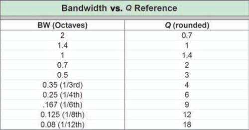
FIGURE 1.17
Bandwidth vs. Q conversion reference (after Rane Corporation, www.rane.com/library.html).

An additional form of filter can be used to create broad flat changes in frequency response. Known as shelving filters, they differ from the parametric by their lack of bandwidth control. The corner frequency sets the range of action and the magnitude control sets the level to which the shelf will flatten out. This type of filter provides a gentle shaping of the system response with minimal phase shift (Fig. 1.19).

FREQUENCY DIVIDERS

The job of the frequency divider (also termed the spectral divider in this text) is to separate the audio spectrum so that it can be optimally recombined in the acoustic space (Fig. 1.20). The separation is to accommodate the physics that makes it impossible (currently) to have any one device that can reproduce the full audio range with sufficient quality and power.

Note: This device is commonly known as an electronic crossover, which is a misnomer. The electronic device divides the signal, which is then recombined acoustically. It is in the

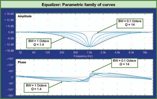
FIGURE 1.18
Standard parametric equalizer curve family.

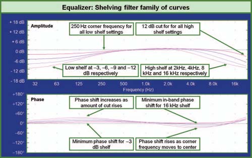
FIGURE 1.19
Shelving filter family of curves.

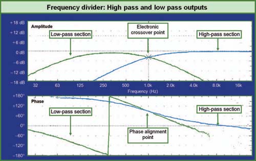
FIGURE 1.20
Frequency divider curve family.

acoustical medium that the “crossing over” occurs, hence the term “acoustical crossover.” This is not just a case of academic semantics. Acoustical crossovers are present in our room at any location where signals of matched origin meet at equal level. This includes much more than just the frequency range where high and low drivers meet, and also includes the interaction of multiple full-range speakers and even room reflections. A central component of the optimized design is the management of acoustic crossovers. Frequency dividers are only one of the components that combine to create acoustic crossovers.

Frequency dividers have user-settable corner frequency, slope, and filter topology. Much is made in the audio community of the benefits of the Bessel, Butterworth, Linkwitz–Riley, or some other filter topologies. Each topology differs somewhat around the corner frequency but then takes on the same basic slope as the full effects of the filter order become dominant. There is no simple answer to the topology question since the acoustic properties of the devices being combined will play their own role in the summation in the acoustical crossover range. That summation will be determined by the particulars of the mechanical devices as well as the settings on the frequency divider. A far more critical parameter than topology type is that of filter order, and the ability to provide different orders to the high- and low-pass channels. Placing different slope orders into the equation allows us to create an asymmetrical frequency divider, an appropriate option for the inherent asymmetry of the transducers being combined. Any frequency divider that can generate up to fourth order (24 dB per octave) should be more than sufficient for our slope requirements.

An additional parameter that can be found in some frequency dividers is phase alignment circuitry. This can come in the form of standard signal delay or as a specialized form of phase filter known as an all-pass filter. The standard delay can be used to compensate for the mechanical offset between high and low drivers so that the most favorable construction design can be utilized. The all-pass filter is a tunable delay that can be set to a particular range of frequencies. The bandwidth and center frequency are user-selectable.

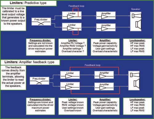
FIGURE 1.21
Predictive limiter scheme (upper). The limiter is calibrated independently of the amplifier. For this scheme to be effective, the limiter must be calibrated to the known voltage gain and peak power characteristics of the amplifier. Changes in the amplifier input level control will de-calibrate the limiter. Negative feedback scheme (lower). The limiter is calibrated to the output of the amplifier. The limiter remains calibrated even with changes in the amplifier level control.

All-pass filters can be found in dedicated speaker controllers and active speakers, where conditions are sufficiently controlled such that the parameters can be optimized.

The all-pass has gained popularity of late as an additional tool for system optimization. There are some promising applications such as the modification of one speaker's phase response in order to make it compatible with another. There is also some exciting potential for LF beam steering in arrays by selectively applying delay to some elements. It is important, however, to understand that such a tool will require much greater skill for practical application than traditional filters. Exotic solutions such as this should not take precedence over the overall task of uniformity over the space. The belief that an all-pass filter tuned for the mix position will benefit the paying customers is as unfounded an idea of any of the single-point strategies. It will be a happy day in the future when we reach a point where we have speaker systems in the field that are so well optimized that the only thing left to do is to fine-tune all-pass delays.

LIMITERS

Limiters are voltage regulation devices that reduce the dynamic range of the signal passing through (Fig. 1.21). They can be applied at any point in the signal chain including individual input channels, output channels, or the post-frequency-divider signal driving a power amplifier. Our scope of interest is limiters that manage the input signal to the power amplifiers in order to provide protection for the loudspeakers. Limiters are not a requirement in the transmission path. If the system is always operated safely within its linear range, there is no need for limiting. This could happen in our lifetime, as could world peace. But unfortunately, we have to assume the worst-case scenario: that the system will be subjected to the maximum level of abuse fathomable, plus 6 dB. Overload conditions are a strain on both the amplifiers and the speakers and have many undesirable sonic characteristics (to most of us). Limiters are devices with a thresholdcontrolled variable voltage gain. The behavior of the device is characterized by its two operating ranges: linear and nonlinear and by the timing parameters associated with the transition between the states: attack and release. The ranges are separated by the voltage threshold and the associated time constants that govern the transition between them. If the input signal exceeds the threshold for a sufficient period of time, the limiter gain becomes nonlinear. The voltage gain of the circuit decreases because the output becomes clamped at the threshold level, despite rising levels at the input. If the input level recedes to below the threshold for a sufficient duration, the “all clear” sounds and the device returns to linear gain.

Limiters may be found inside the mix console where the application is principally for dynamic control of the mix, which falls outside of our concern for system protection. Additional locations include the signal-processing chain both before and after active frequency dividers. A limiter applied before frequency division is difficult to link to the physics of a particular driver, unless the limiter has frequency-sensitive threshold parameters. The most common approach to system protection is after the frequency divider, where the limiters are charged with a particular driver model operating in a known and restricted frequency range. Such limiters can be found as stand-alone devices, as part of the active frequency divider (analog or digital) or even inside the power amplifier itself.

Where does the limiter get its threshold and time constant settings? Most modern systems utilize factory settings based on the manufacturer-recommended power and excursion levels. There are two principal causes of loudspeaker mortality: heat and mechanical trauma. The heat factor is managed by RMS limiters, which can monitor the long-term thermal conditions based upon the power dissipated. The mechanical trauma results from over-excursion of the drivers, resulting in collision with the magnet structure or from the fracturing of parts of the driver assembly. Trauma protection must be much faster than heat protection; therefore the time constants are much faster. These types of limiters are termed peak limiters. Ideally, limiters will be calibrated to the particular physics of the drivers. If the limiters are not optimized for the drivers, they may degrade the dynamic response with excess limiting or possibly fail (insufficient limiting) in their primary mission of protection. The best designed systems incorporate the optimal balance of peak and RMS limiting. This is most safely done with the use of amplifiers with voltage limits that fall within the driver's mechanical range and peak limiters that are fast enough to prevent the amplifier from exceeding those limits or clipping. The results are peaks that are fully and safely realized and RMS levels that can endure the long-term thermal load.

A seemingly safe approach would be to use lower-power amplifiers or set the limiting thresholds well below the full capability so as to err on the side of caution. This is not necessarily the best course. Overly protective limiters can actually endanger the system because the lack of dynamic range causes operators searching for maximum impact to push the system into a continual state of compression. This creates a worst-case long-term heat scenario as well as the mechanical challenges of tracking square waves if the amplifiers or drive electronics are allowed to clip. The best chances of long-term survival and satisfaction are a combination of responsible operation and limiters optimized for maximum dynamic range.

Limiters can be split into two basic categories: predictive or negative feedback loop. Predictive limiters are inserted in the signal path before the power amplifier(s). They have no direct correlation to the voltage appearing at the amplifier outputs. Therefore, their relationship to the signal they are managing is an open variable that must be calibrated for the particulars of the system. For such a scheme to be successful, the factors discussed above must become known and enacted in a meaningful way into the limiter. Such practices are common in the industry. I do not intend to be an alarmist. Thousands of speakers survive these conditions, night after night. The intention here is to heighten awareness of the factors to be considered in the settings. Satisfactory results can be achieved as long as the limiters can be made to maintain an appropriate tracking relationship to the output of the power amplifiers. Consult the manufacturers of speakers, limiters and amplifiers for their recommended settings and practices.

Required known parameters for predictive limiters:

■ Voltage limits (maximum power capability) of the amplifier

■ Voltage gain of the amplifier (this includes user-controlled level settings)

■ Peak voltage maximum capability of the loudspeaker

■ Excursion limits of the loudspeaker over its frequency range of operation

■ Long-term RMS power capability of the loudspeaker?

Negative feedback systems employ a loop that returns the voltage from the amplifier terminals. This voltage is then used for comparison to the threshold. In this way the voltage gain and clipping characteristics of the amplifier are incorporated into the limiting process. This is common practice in dedicated speaker controllers and can afford a comparable or greater degree of protection with lesser management requirements for the power amplifiers; e.g., the amplifier input level controls may be adjusted without readjusting the limit threshold.

DEDICATED SPEAKER CONTROLLERS

Many speaker manufacturers also make dedicated speaker controllers (Fig. 1.22). The controllers are designed to create the electronic-processing parameters necessary to obtain optimal performance of the speaker. The parameters are researched in the manufacturer's controlled environment and a speaker “system” is created from the combination of optimized electronics and known drivers. The dedicated speaker controller contains the same series of devices already described above: level setting, frequency divider, equalization, phase alignment, and limiters, all preconfigured and under one roof. The individual parameters are manufacturer- and model-dependent so there is little more that needs be said here. This does not mean that equalizers, delays, and level-setting devices can be dispensed with. We will still need these tools to integrate the speaker system with other speakers and to compensate for their interaction in the room. We will, however, have reduced the need for additional frequency dividers and limiters and should have a much lighter burden in terms of equalization.

Two recent trends have lessened the popularity of these dedicated systems in the current era. The first is the trend toward third-party digital signal processors (DSPs). These units are able to provide all of the functionality of the dedicated controllers, usually with the exception of negative feedback limiters. Manufacturers supply users with factory settings that are then programmed into the DSP. These tools have the advantage of relatively low cost and flexibility but the disadvantages include a lack of standardized response since users of a particular system may choose to program their own custom settings instead of those recommended by the manufacturer. There is also considerable latitude for user error

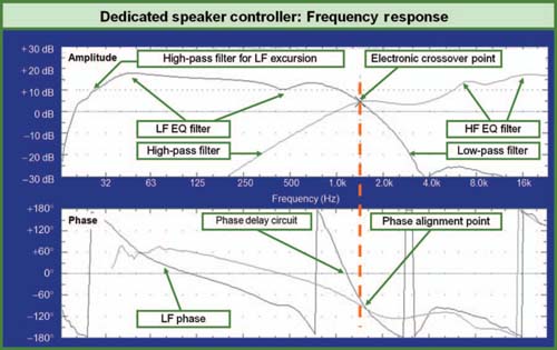
FIGURE 1.22
Frequency and phase response of an example two-way dedicated speaker controller.

since the programming, copying and pasting of user settings is often poorly executed even by the best of us. The second trend is toward completely integrated systems, inclusive of the amplifier in the speaker cabinet.

ACTIVE SPEAKERS

The ultimate version of the dedicated speaker controller is this: a frequency divider, limiter, delay line, level control, equalizer, and power amplifier in a single unit directly coupled to the speaker itself. This type of system is the self-powered speaker, also termed the “active” speaker. Active speakers operate with a closed set of variables: known drivers, enclosure, known physical displacement, maximum excursion, and dissipation. As a result, they are designed to be fully optimized for the most linear amplitude and phase response over the full frequency range and to be fully protected over their full dynamic range. Active speakers, like power amplifiers, have an open polarity variable, since they are electronically balanced at the input and moving air at the output. Since most active speakers came on the market after industry polarity standardization, it would be rare to find a nonstandard system.

From our design and optimization perspective, active speakers give us unlimited flexibility in terms of system subdivision; i.e., the number of active speakers equals the number of channels and subdivision options. Externally powered speakers by contrast may, for economic reasons, often share up to four drivers on a common power amplifier channel and thereby reduce subdivision flexibility.

There will be no advocacy here as to the superiority of either active or externally powered (passive) loudspeakers. We will leave this to the manufacturers. The principal differences will be noted as we progress, since this choice will affect our optimization and design strategies. In this text, we will consider the speaker system to be a complete system with frequency divider, limiters, and power amplifiers inclusive. In the case of the active speaker, this is a physical reality, while in the case of the externally powered system, the components are separated. The techniques required to verify the proper configuration of these two different system types will be covered in Chapter 11.

Line level interconnection

This subject is often the source of confusion due in large part to practices that were developed in the distant past when our audio world was filled with transformer inputs and outputs connected to vacuum tubes. In that case, the line level interconnection was an electrical power transfer (as is still the case with an amplifier and speaker). The line level power transfer strategy relied upon matched impedance between input and output and was based upon the old telephone transmission standard of 600Ω. This approach was critical for the very real power transfer needs between the primitive carbon button transducers on either end of the telephone line. The line level devices of modern professional sound systems are active and do not operate under these restrictions and need transfer only negligible amounts of power. The signal transfer is effectively reduced to voltage only; hence the term voltage source describes the transmission system between line level devices. A voltage source is capable of signal transfer that is virtually without loss as long as the driving impedance is very low compared to the receiver. Hence, the modern system seeks an impedance mismatch in direct contrast to the practices of the past.

 

The amount of loss over the line depends upon the combined impedance of the output relative to the combined impedance of the cable and the input. We will now apply this formula to the typical system shown previously in Fig. 1.16 (neglecting the cable impedance for the moment).

The combined 10 kΩ input impedance and 150Ω output impedance are divided by the 10 kΩ input impedance (10,150Ω/10,000Ω) to create a ratio of 203:200, a loss of 0.13 dB. Each additional input fed by this output would reduce the input impedance seen by the output device. Each parallel addition increases the loss by an additional 0.13 dB increment. Therefore we need not be concerned about splitting line level output signals to multiple sources until the number of inputs becomes quite large. The remaining factor is the cable impedance. Cable impedance is a product of the combined effects of cable DC resistance and AC reactance, which comes in the form of cable capacitance and inductance. The reactive properties are frequency-dependent. Cable capacitance acts as a low-pass filter while inductance acts as a high-pass filter. The DC resistance acts as a fullrange attenuator. The band pass combination of the cable reactance can be a cause of concern if we are running long lines. Everything you ever wanted to know on this subject (and more) can be found in Audio System: Design and Installation by Phil Giddings. According to that text, as long as our runs are less than 305m (1000 ft), there is no reason for concern. An additional consideration regarding the line level interconnection loss: it is the easiest loss to compensate. If this were not the case, we would never have been able to communicate via telephones. Overcoming this loss requires a voltage gain boost, which is readily available to us in the form of active level controls. The principal side-effect would be a rise in the noise floor. This is not to say that such a loss is recommended—only that the interconnection loss in line level systems is far less critical than in speaker lines, where a 6 dB drop would mean a loss of 75% of your power. The difference is that line level systems are transferring negligible power. They are transferring voltage, which is a simpler matter to restore.

The input stage is balanced in order to reject noise that is injected onto the cable driving the input. The term balanced line refers to the wiring configuration that uses two signal conductors and one common (which may or may not be connected to chassis or ground). The two conductors always contain identical copies of the input signal but are reversed in polarity from each other. The two signals are fed into a “differential” input stage, which amplifies only signals that are unmatched—which is exactly the case with our input signal. Any noise that has entered the cable (electromagnetic interference and radio-frequency interference being the most typical) will be found equally in both conductors and will be canceled by the differential input. This result is termed “common-mode rejection” for its ability to suppress induced signals.

The input section may have a level control, which will determine the drive level into the processing module. Once the processing is completed, we proceed to the balanced push–pull output stage. The name comes from its function to prepare a balanced differential output signal: two identical signals, one of which is reverse polarity. As in the input stage, a level control may accompany this stage. Additionally input and/or output meters may be provided to monitor levels. One might assume that the signal is unity gain throughout the internal gain structure of the unit if the input and output level controls are put to their nominal settings. This is not necessarily the case. The overall voltage gain can be anything, and there may be internal stage gains and losses that affect the dynamic range. In short, any active device with multiple gain stages will need to have its dynamic range verified in its various configurations. This verification process is outlined in Chapter 11.

ACTIVE BALANCED

There is a variety of interconnection wiring schemes used in the industry. We will touch on this only briefly to discuss the most common schemes found for our usual signal path. The most common wiring scheme is, of course, not necessarily the best. This scheme ties the balanced inputs and outputs directly together along with the common (shield) as happens with a direct connection through a three-pin XLR cable. The drawback of this scheme is the ground loop path that is created by the shield connection. An alternate scheme is able to provide shielded balanced operation without introducing a ground loop. The shield is connected on the source side only. This removes the ground loop. These schemes are shown in Fig. 1.23.

TRANSFORMER BALANCED

A balanced transformer can be substituted for the active input with advantages in isolation between the systems. The degradation effects of transformers are well documented but there are some applications where the isolation advantages outweigh the degrading effects. This configuration is shown in Fig. 1.24.

UNBALANCED

There are occasions when the equipment provided does not have balanced inputs or outputs. In such instances, we will want to preserve the performance of balanced lines as much as possible. Wiring schemes have been developed that most closely approximate balanced line performance. These are shown in Fig. 1.25. When an unbalanced output drives a balanced input, the differential inputs are fed by the signal and common respectively. This allows for the common-mode rejection to suppress any interference that

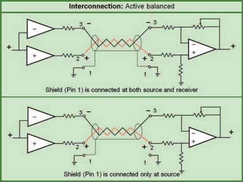
FIGURE 1.23
Top: Typical active balanced line interconnection (possible ground loop). Bottom: Improved active balanced line interconnection (no ground loop because the shield is not connected to the input ground) (after Giddings, 1990, pp. 219–220).

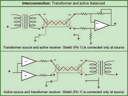
FIGURE 1.24
Top: Balanced transformer output interconnection to active balanced input. Bottom: Active balanced line interconnection to balanced transformer input (after Giddings, 1990, pp. 221–223).

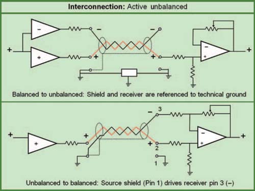
FIGURE 1.25
Top: Active balanced output interconnection to active unbalanced input. Note that the commons must be linked by a technical ground. Bottom: Active unbalanced output interconnection to active balanced input (after Giddings, 1990, pp. 226–229).

is injected into the line. The success of this scheme will depend upon the isolation between the grounds of the two devices.

Important note: Unbalanced interconnections are one of the most common sources of polarity reversals. Verify that the connection is made across the non-inverting source and receivers terminals.

In cases where an active balanced output drives an unbalanced input, the system will not have improved performance over an unbalanced-to-unbalanced configuration. The reverse polarity side of the push–pull output will not be used and the shield connection will be made at only one end. The ground connection will need to be made through a common technical ground rather than through the shield where a loop would be introduced.

Speaker level devices—power amplifiers

Speaker level transmission moves us into the realm of real power. The speaker level voltages run higher than line by a factor of 10:1 or more, reaching 100 V_RMS. But that ratio pales in comparison to the difference in current levels, which can easily reach 250:1. This translates to real power. The minuscule power dissipation of a line level output gives way to the 1000 watts transmitted from a speaker level output. We are no longer able to operate with the one-dimensional voltage frame of mind. Speaker level transmission requires us to work with the more complex properties of electrical power.

In our professional audio transmission application, the amplifier is the source of current and voltage, and the speaker and cabling are the resistance. The motion of the speaker coil tracks the voltage of the audio waveform. The amplifier supplies current as dictated by the output voltage and the voice coil impedance and sets the speaker in motion. Speakers are not unlike a typical teenager: they are resistant to change and require a great deal of motivation to be moved from their natural state of rest. Current provides the motivation, while voltage guides the direction. A positive voltage will cause the speaker to move in one direction while a negative signal reverses the motion. The extent of the speaker movement (its excursion) is proportional to the voltage component of the waveform. The supplied current must be high enough to move the low-impedance speaker coil in the magnetic structure, thereby providing the required mechanical force to keep the speaker on track with the waveform.

POWER AND IMPEDANCE

Component power amplifiers have several key parameters from the design viewpoint: the maximum power (wattage) and the minimum impedance. The maximum wattage matches the amplifier operating range to the recommended range of the speaker. Amplifiers have fairly standardized ratings in these terms, while the speaker specifications are much less clear cut. The matching of amplifier to speaker is best accomplished by following the guidelines given by the speaker manufacturer.

The minimum impedance governs how many speakers can be loaded onto the output terminals before fire accompanies the signal. Most amplifiers claim to be able to operate down to 2Ω. This allows up to four 8Ω speakers to be connected in parallel. The temptation is high to load an amplifier down to 2Ω because we are able to drive the maximum number of speakers for the price of a single amplifier. This is rarely done for two reasons. First, the sound quality is seriously degraded due to the reduced damping factor control of the load that occurs when amplifiers must deliver such massive amounts of current. Second, the amplifiers tend to live very short lives.

The minimum standard operating impedance for component amplifiers is 4Ω. This will take two 8Ω drivers or four 16Ω HF drivers. Since an amplifier costs the same whether you use it at 8Ω or 4Ω the second speaker is essentially driven for free. In the case of HF drivers, you get four amplifier drivers for the price of one. This is serious money, but it leads to serious compromise by limiting system subdivision. This is the “econΩic” factor of component amplifiers. Our designs will need to be defended against “value engineering” that forces us to operate multiple drivers at matched levels (Fig. 1.26).

POLARITY

Amplifiers take balanced line level signals in and put unbalanced speaker level signals out. Therefore, the “hot” terminal at the output must be matched to one of the two active signals at the input. Those of us with gray hair (or none at all) will remember the decades of Audio Engineering Society indecision on a standard for the question of pin 2 or pin 3 “hot.” At the 1985 AES convention in Los Angeles, a frustrated amplifier manufacturer distributed “AES spinners” with various “pin 2 hot” and “pin 3 hot” sectors arrayed in the circle. And the winner is … pin 2. Any amplifier made later than the late 1980s will be pin 2 hot (Fig. 1.27).

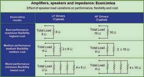
FIGURE 1.26
The considerations of impedance, performance, and cost related to speaker loading of the power amplifier.

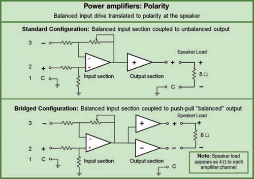
FIGURE 1.27
Flow block of amplifier polarity for standard and bridged mode configurations.

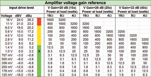
FIGURE 1.28
Amplifier voltage gain reference chart.

VOLTAGE GAIN

Voltage gain is a measure of output voltage related to input voltage. There is much confusion regarding this specification because power amplifier input drive is specified in volts, while the output is in watts. The input and output voltages rise together in a fixed linear gain relationship until clipping is reached. That fixed gain ratio is termed the amplifier voltage gain. Clipping is the point where the output voltage can no longer continue to track the input due to limits in the voltage rails that feed the output transistors. If the amplifier is of professional quality, the clip voltage will be the same for either 8 or 4Ω speaker loads. Therefore, the maximum wattage is derived from the amount of voltage delivered to the load, with the lower-impedance load receiving more wattage for the same voltage.

Manufacturers of power amplifiers muddy the waters on voltage gain by using three differing methods of specifying this parameter: log voltage gain (dB), linear voltage gain (X), and sensitivity (input voltage to reach output clipping).

The linear and log versions are easily related using the 20 × log formula (see Fig. 1.10); e.g., a gain of 20× (linear) is equivalent to 26 dB (log). Sensitivity is more complicated, since it must be evaluated on a case-by-case basis. Sensitivity specifications state the input voltage that will bring the output to onset of clipping. To derive a voltage gain from this, we will need to know the output clip voltage. If the amplifier clips at 10 V and the sensitivity is 1 V, then the amp has 20 dB (10×) voltage gain; e.g., 200 W@8Ω amplifier with a sensitivity of 1 V has a voltage gain of 40× (linear), or 32 dB(log) (Fig. 1.28).

Here is where it gets confusing. Some manufacturers use a standard sensitivity for all amplifiers, regardless of maximum power rating. A 100 W and a 400 W model will both reach full power when driven at the input level of, for example, 0.775 V. This is done by giving the amplifiers 6 dB (2×) difference in voltage gain. Other manufacturers offer standard voltage gains. In those cases, the 400 W amp will require 6 dB more drive level to reach full power. Still others can't make up their mind and change from model to model (Fig. 1.29).

Which is better? A standard drive level that brings all amps to clipping, or a standard voltage gain that has all amps tracking at the same voltage level?

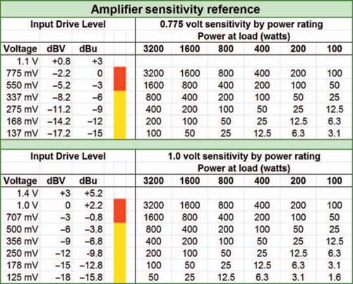
FIGURE 1.29
Amplifier sensitivity reference chart.

The most important factor is that the gain be known. If the amplifiers are sensitivitybased, we can deduce their voltage gain. If they are voltage-gain-based, the job is done for us. Either way, they can be made to work sufficiently by adjustment of the amplifier level controls.

The answer to which is better lies in two places: the frequency dividers and the limiters.

When we have frequency dividers ahead of the amplifier, the signals will need to be recombined acoustically. If amplifiers have matched voltage gain, the job of setting the acoustical crossover is made much easier. For example, if we are using a dedicated speaker controller, the device is designed with the assumption of matched amplifier gains. If the gains are not matched, then the acoustical crossover settings will not be transferred at the intended relative levels, causing a shift of crossover frequency (see Fig. 1.30). This is also true if we are using factory-recommended settings programmed into a DSP.

Why would the voltage gains be unmatched? This would occur in a sensitivity-based amp with high and lower drivers being driven by amplifiers with different maximum power. As in the example above, a 400 W low-driver amp paired with a 100 W HF driver amp would have 6 dB of difference in gain at the crossover if the amps were sensitivity-based. A 12 dB/octave crossover point could shift by half an octave upward.

The second factor is related to the use of limiters. Limiter action is based upon voltage level. Estimates of the power (wattage) at the speaker are based upon the voltage that is seen by the limiter circuit. If the voltage gain of the amplifier is unknown, the limiter is uncalibrated. An uncalibrated limiter will either decrease the dynamic range unnecessarily or not provide the needed protection.

LEVEL CONTROLS

An additional case of nonstandardization in the amplifier market is the various level control markings. As if it is not enough to have us confused about voltage gains, let's add level controls with meaningless markings. It is not unusual to hear that the amplifiers have been set to “three clicks down.” Huh? Marking schemes include: dB relative to maximum voltage gain (linear or log), blank with tick marks, the numbers 0 to 10, and there is at least one manufacturer that displays dB voltage gain. If a system is made up entirely of one model of power amplifier, it is possible to use the markings for some relative calibration. If it is in “clicks” the calibration only holds if all are at the same click or if the clicks actually change the level in uniform dB increments. But since the different speakers have different power needs, there is very little chance that a single amp will suffice. Once we introduce different models, we have opened a Pandora's box of unrelated scales. Help!

It is also worth noting that the amplifier level control does not reduce the maximum power capability of the amp as one might believe from listening to too much audio folklore or watching the film This is Spinal Tap. Turning the level control down merely resets the drive level required to reach full power. Resetting the start position of the accelerator does not add horsepower to our engine. It only changes the position of our foot relative to our speed. So it is with amplifier level controls. As long as the amp level control is not turned down so low that the drive electronics will not be able to clip the amp, we are fine. The reaction of most engineers has been to fear the lack of calibration in amplifiers and impose an edict of “all amps set to fully open.” This is a regrettable yet understandable consequence of the lack of standards. It does, however, reduce our optimization options regarding relative level between system components. And it increases audible speaker system noise.

Speaker level interconnection—speaker cables

Relatively speaking, the connection between the amplifier and speaker is another case of a low-impedance output driving a high-impedance load. While 8Ω would not seem to qualify as a high-impedance load, it is when compared to the extremely low 0.1Ω output impedance of the amplifier. This familiar impedance scaling allows the amplifier to drive the speaker reliably. The low overall impedance allows lots of current to flow, and therefore lots of power.

Speaker cable runs are a different story than line level cables. They are prone to substantial amounts of resistive loss because the impedance of the cable can become significant in proportion to the speaker load. The loss rate depends primarily upon three factors: cable length, conductor diameter, and load impedance. The loss increases with the cable length. Decreasing load impedance and cable diameter also increases the loss (Fig. 1.30).

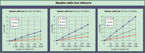
FIGURE 1.30
Charts of speaker level cable transmission loss (after Giddings, 1990, pp. 333–335).

We have the option of running single or multiple cables in cases where multiple speakers are driven from a single amplifier channel. This is a trade-off of the cost of additional cable against the benefit of reduced resistive losses. The cable loss charts can help to evaluate the potential benefits of splitting into parallel runs. Bear in mind the cost of the power amplifier and the fact that the loss of 3 dB is equivalent to half its power.

Speaker cable losses are challenging to measure directly, due to the high-voltage levels and the fact that the speaker must be attached to the amplifier to properly monitor the load effects. In practice, we will usually make do with measuring the results in the acoustic response of the installed speaker and adjustments for unmatched responses made at the power amplifier level controls; e.g., two matched speakers with matched coverage areas that are run from an amp room that is much closer to one of them.

A final note regarding speaker cable impedance losses: Since the loudspeaker load does not have a constant impedance over frequency, the losses will vary over frequency. The specified impedance for speakers is normally the lowest impedance in its operating range and therefore the worst-case scenario for losses. Other frequency ranges will have higher impedance and therefore less loss, resulting in a modified final frequency response.

DIGITAL AUDIO TRANSMISSION

Digital audio devices

Up to this point, we have considered digital audio only in the context of a processing module inside an analog device. In such cases, the unit functions as a line level analog device in terms of its gain structure and interconnection properties. When the input signal enters our transmission system in digital form, the interconnection properties discussed previously no longer apply. Forget about line level, impedance, and balanced lines. In our discussion of line level, we saw that current considerations were of minimal importance. Now even voltage is out. It has been converted into numbers. Welcome to the information age.

Digital audio transmission operates under a new set of rules. In fact, the term transmission as we have been using it is not fully applicable to digital audio. Analog transmission requires a medium, and digital audio is medium-independent. Whether the digital signal moves through optical fiber, wire, or wireless Internet will not affect the frequency response, as with all other media. Digital audio transmission is a data transfer. If the data is transferred faithfully, we will have a matched copy at both ends of the transference. This is never the case in analog transmission through a medium, which always has a loss.

Trap 'n Zoid by 6o6

Trap 'n Zoid by 6o6

This is not to say that there are no concerns regarding data transmission. There are a great number of opportunities for data damage. If it becomes corrupted, it is unlikely to manifest itself as something that we can recognize as an “audio” problem. The more likely outcomes of digital transmission errors are no audio, audio from the planet Zircon or, worse yet, maximum level noise.

The world of digital audio is evolving rapidly. We are witnessing a steady erosion of the portion of the audio transmission path left in the analog domain. It began with delay lines. Yes, there actually were such things as analog delay lines. Next came digital equalizers, frequency dividers, and onward. Is there any doubt that in the future we will have an analog-to-digital (A/D) conversion at the beginning of the transmission path and remain digital until the last possible link in the chain to our analog ears? These developments, however significant, do not change our basic mission: monitor the transmission and enact corrections as required. Since most of the damage is done in the acoustical world, the digital age offers us superior flexibility of corrective tools, but not a new world order.

BANDWIDTH

The digital audio bandwidth is not determined by capacitance and inductance, but rather by the digital sample frequency. The most common digital transmission sample frequencies are 44.1, 48, and 96 kHz with 192 kHz becoming more common. The frequency range upper limit is no more than half of this sample rate. We might wonder why we would need anything more than bandwidth above 20 kHz. The reason is that the sharp filters used to limit the upper range in digital systems cause phase shift below their corner frequency. As the corner frequency rises, the amount of phase shift within our hearing range decreases.

DYNAMIC RANGE

The dynamic range is determined by the bit resolution. The analog signal is encoded voltage values, which are stored as bits. Each represents a voltage threshold that is half of the previous. The top of the dynamic range is the highest number and is termed full-scale digital. It is important to note the relationship of full-scale digital-to-analog voltage is not fixed and can range from +20 dBV down to 0 dBV. The number of bits, i.e., the resolution, determines how far down we go before the encoding process no longer differentiates the signal. Each additional bit gives us an additional 6 dB of signal to work with at the bottom of the range. The AES/EBU standard is 20 bits, which yields a maximum dynamic range of around 120 dB. AES3-2003 allows 24 bits at 96 kHz sampling rate. It also allows 16 bits at 32 kHz.

From the viewpoint of the optimized design, there is little reason for us to go into extensive detail on digital audio. There are no equalization or level-setting decisions that one would approach differently, nor delay settings (provided we have compensated for the latency issues). From an operational standpoint, the analog and digital worlds are similar. We must keep the signal within the linear operating range and out of the noise. The fact that all of the digital settings can be stored and recalled (and erased) is an operational convenience, not an optimization factor.

DEVICE LATENCY

One of the most noticeable differences between digital and analog devices is the length of the latency period. Latency is the transit time of the signal through an electronic device, a full bandwidth delay between the input and output. Analog latency is measured in nanoseconds (10⁻⁹s), which is so small that it is considered negligible compared to digital audio, which is several milliseconds at best. There are a variety of causes of latency including A/D conversion and memory buffering in digital signal-processing devices. Our focus here is on the effects, not the cause. We need awareness of where latency may occur so that we may compensate for it during the optimization process.

Digital audio interconnection

Digital audio is an encoded representation of the waveform. The analog waveform is a continuous linear function: there are no breaks in the cyclical movement from ambient state to the high- and low-amplitude extremes. Digital audio is a finite series of incremental steps that are assembled to create a rendering of the continuous waveform.

Principal forms of professional digital audio interconnection:

1. AES/EBU (a standard also known as AES3): This encodes two channels of audio into a single data stream (or connection). It supports up to 24-bit sampling with preferred sampling frequencies of 44.1, 48, and 96 kHz. The standard connection is made with a shielded pair cable and XLR connectors. The signal is balanced and requires a cable with a 110Ω characteristic impedance. Optical transmission is accomplished by the F05 connector. S/P DIF is an unbalanced consumer variant.

2. Network: There are various network protocols, the most common being Ethernet/ Cobranet. Networked interconnections follow the standard wiring practices of the computer industry. “Thank you for calling the technical support hot line. Your call is important to us …”

3. Proprietary: Manufacturer-specific interconnection that does not conform to any standard (or theirs alone) and only connects to their own equipment. See manufacturer's specifications for details.

Each of the transmission interconnection paths has limited cable length. The principal factor limiting the length is the type of cable used. Unlike cables used for analog signals, cables used for digital signals are built to have controlled impedances, and it is essential that a cable has the proper characteristic impedance that matches the system being used. By driving these cables properly at the transmitter end, and terminating them correctly at the receiver, they will move the digital data streams around safely. All of this driving and receiving is built into the equipment we are using, so all we have to do is supply the correct cable type. The routine practice of splitting signals in the analog world is not advisable for digital interconnections. Very short cable runs may continue to work in such cases, but this is a risky practice.

The data stream is a series of binary states: “1 s” and “0 s” that are represented by voltage levels. There is no tolerance for half states. The receiving end of the digital transmission line must differentiate the 1 s from the 0 s, a task that is made more challenging as distortion of the signal increases. Using the wrong type of cable results in distortion that limits the distance the signal can travel before becoming unreliable. As the distortion increases, the decoder can no longer reliably discern the data states and errors are generated that can result in dropouts and audible distortion.

NETWORK LATENCY

Transmission of analog electronic signals travels in a continuous stream at two-thirds the speed of light. Therefore, in analog systems, there is little need to worry about combining systems with different lengths of cable unless these are extremely long runs. In practice, with such cases, the frequency response degradation from the long runs is more of a concern than the latency and therefore most runs of such length are made via digital transmission.

Digital audio is transmitted in packets of data. The speed of the transfer is networkdependent. The interconnection between devices and over digital audio networks is an area full of opportunities for differences in latency delay. Interconnected systems may have a particular latency between local devices within a proprietary system (such as expansion channels of a console or signal processor) and a different latency when connected to other systems. Optical conversion systems, AES, TCP/IP, Ethernet, and other transmission networks all have configuration-dependent latencies. In short, we will have to measure these when installed in order to ensure compatibility between any summed signals from alternate paths. The verification procedure is detailed in Chapter 11.

ACCESS TO INFORMATION

The analog audio world contains multiple interconnections. This is a mixed blessing. On the negative side are the myriad opportunities for interconnection errors, ground loops, and component failures. On the other side is the fact that we can monitor the signal at various points along the way, re-route it if necessary and, most important in our case, we can measure it. Digital audio systems in general, and networked systems in particular, tend to leave us unable to monitor the signal en route. The reason is simple: to bring a signal out of the system requires a digital-to-analog converter, a connector, and so on. This drives the cost up. Since our interest here is to design systems that can be fully optimized it is vital that the signal-processing parameters, i.e., equalization, delay, and level setting, be visible to our analyzer. Any system that leaves us fenced out of the signal path is less able to be fully optimized, and is therefore less desirable. The user interface renderings of EQ, level, and delay should never be trusted on blind faith. They must be measured. The criteria for access to measurement are detailed in Chapters 10 and 11.

ACOUSTIC TRANSMISSION

Power, pressure, and surface area

Acoustic power operates under the same conditions as the electrical power discussed previously, with analogous aspects and also is measured in watts. Sound pressure is analogous to voltage, and is measured in dB SPL (sound pressure level). Surface area is like current. The acoustic watt could be the product of high pressure in a small area or low pressure in a large area. To illustrate this, let's consider a favorite source of acoustic power: fireworks.

An explosive charge pressurizes the air in direct contact with burning powder and propagates spherically outward from the point of origin. The amount of acoustic energy (power) created by the explosion remains constant as the sound wave moves outward from the source. The outward movement stretches the surface area of the wave. Since the quantity of energy is fixed, it is not possible to maintain the same pressure level while expanding the surface area. As the surface area increases, the pressure decreases proportionally, leaving us with the original quantity of acoustic energy. Does this mean that it does not matter how close we are to the explosion? Of course not. If we get too close we will damage our ears, or worse. But the damage is not due to the acoustic power. It is a consequence of excessive sound pressure.

Our ears are sound pressure sensors. There is no way for us to sense acoustic power. We would have to be spread over the entire surface area to experience it. We cannot detect the presence of sound anywhere else but our ears. We only hear reflected sounds because their paths lead them to our ears.

The quantity of acoustic power a device generates is of interest to loudspeaker designers but few others spend time considering it. A loudspeaker, like the fireworks charge, has a fixed amount of acoustic power at its source. From the perspective of audio engineers, the critical metric for sound system performance is sound pressure. How much sound pressure level can we deliver to our ears? However, if we are to concern ourselves with creating the desired sound pressure at locations other than the exclusive confines of the mix position, we need to be very conscious of the surface area aspect of sound propagation. As mentioned earlier, sound propagates spherically from the acoustic source. If the audience members are all located equidistant from the source, they will experience the same sound pressure. If not, it will be necessary to create an asymmetrical acoustical power source that can maintain constant sound pressure level into the locations that are more distant. This is done by steering the sound so that the surface area is decreased, thus allowing for higher pressure at a given distance. Our choice is simple. Either we construct our listening environments such that all members of the audience are equidistant or we learn how to steer the sound.

We are finished with the concept of acoustic power. From here forward, we will focus on sound pressure level spread over the surface area. It is common, however, for audio engineers to use the term “power” and SPL interchangeably. To the extent that this may occur in this text, please bear in mind that we are referring to pressure.

As sound propagates away from the source, the SPL decreases at a rate of 6 dB for each distance doubling (Fig. 1.31). This rate holds for a source in a free-field (reflection-free) acoustic environment. This loss rate is known as the inverse square law. The presence of reflections reduces the rate of loss as the secondary source is added to the direct sound. The level changing effects of reflections are highly variable over frequency and location and therefore no simple formula is applicable to reverberant environments. An accurate characterization will require on-site measurement. Considering we will probably never do a show in free-field, this is a notable limitation to our dB SPL prediction capability. It will, however, serve us well to be mindful of the free-field loss rate while making predictions and measurements. Taking the free-field rate as a standard allows us to discern the strength of the reflections and other factors when the losses differ from the standard rate. For our purposes then, it is assumed that the loss will occur at the free-field rate unless other specified (Fig. 1.32).

Environmental effects: humidity and temperature

There are additional factors above and beyond the inverse square law that affect transmission loss. Air is a nonlinear transmission medium, i.e., the high frequencies are attenuated at a greater rate than lows. The highest frequencies are the most strongly affected with the losses gradually decreasing as frequency falls. The losses accumulate over distance; therefore concerns

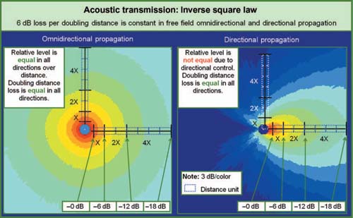
FIGURE 1.31
Spherical sound propagation: (left) omnidirectional source; (right) directional source.

in this regard become quite significant in long throw applications. In the near field, a speaker's very-high-frequency (VHF) range extension is at its maximum. As we move further away, the VHF area will become low-pass-filtered. As more distance is traveled, the corner frequency of the filter action moves downward.

Most audio engineers are familiar with the environmental effects on their sound systems. The sun goes down and the system seems to undergo radical changes in the HF range. Battle stations.

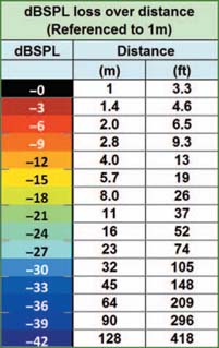
FIGURE 1.32
Sound propagation loss over distance.

There are three factors whose combined effects create the values of transmission loss through the medium of air: distance, humidity, and temperature. These mix together in some unexpected combinations, much like weather in general. That said, there are two prevalent trends that will apply to the huge majority of applications. The first is that as humidity rises, HF transmission improves (i.e., the loss rate decreases). This holds over temperature for humidity levels above 40%, which will cover any indoor location and any but the most arid outdoors venues. The losses resemble a fairly steep high-cut filter, with the corner frequency moving down as humidity falls. The second trend involves temperature and simplifies as follows: within the humidity range cited above, the loss rate is highest around room temperature (20°C) and increases as temperature either rises or falls around this standard. At humidity levels of 30% and below the filtering effects change character and the exceptions become numerous and are best understood by viewing the loss values chart found in Fig. 1.33.

Weather conditions can have discernible effects upon the directional transmission of sound as well. Temperature gradients can separate the atmosphere into layers, thereby providing a refractive component to the sound transmission as it encounters the change in temperature. This response is well known in the field of underwater acoustics, where the hunting of submarines is made more difficult by the refractive effects of layers of water at different temperatures. In airborne sound, this is often experienced as the arrival of a

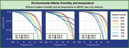
FIGURE 1.33
Transmission loss over a distance of 100 m due to air absorption over temperature and humidity at: (left) 10°C, (center) 20°C, (right) 30°C. Conversions are approximately 50°F, 68°F, and 86°F at a distance of 318 ft (courtesy of Meyer Sound Laboratories Inc.).

distant sound at a much higher than expected level, such as a train whistle on a foggy night. In the world of outdoor concert sound, this can cause unexpected vertical redirection of the speaker system transmission.

It is very difficult to ascertain the independent action of these factors in the field. Fortunately, there is also little need to precisely do so. Because the filter action occurs almost entirely in the VHF region, its effects are among the easiest to identify with an analyzer or by ear. The solution is the same regardless of its precise cause.

Acoustic transmitters: loudspeakers

We have reached the end of the electronic transmission chain: the loudspeaker. The role of the speaker is delivery of the original transmission to the listeners. In the ideal world, we might be able to do the job with a single full-range speaker capable of creating the surface area shape that spreads even SPL over the listening area. There are a limited number of shapes that a single speaker can create. Therefore, the likelihood of a perfect fit is poor. Most applications have complex shapes that will require multiple speakers to evenly spread the SPL to conform to the particular shape. But before we can begin to attempt this, we will need to investigate the transmission characteristics of a single loudspeaker and create a framework to evaluate its behavior.

The first item to establish is that we will not discuss loudspeakers at all. We will only discuss loudspeaker systems. This book is not targeted at the research scientists of professional loudspeaker manufacturers. Nor is it intended to aid garage scientists who wish to find the ultimate mix of components and turn lead into gold. The age of audio alchemy is long gone (Fig. 1.34). We use engineered systems, i.e., speakers in tuned enclosures with documented characteristics, repeatable construction, and professional quality standards.

Let's begin with a generic specification list of the expected characteristics of loudspeakers.

Professional loudspeakers system generic specifications:

1. Amplifier(s) shall be capable of driving the system to full SPL without input stage overload.

2. Systems shall have known operational limits. Amplifiers and limiters shall be calibrated such that the speakers may be operated within the limits without fear of damage. System shall be self-protecting.

3. System shall be capable of reaching maximum SPL with graceful overload characteristics.

4. System shall be low noise, with dynamic range >100 dB.

5. Frequency range of 70 Hz to 18 kHz to be covered as a two-way system (minimum), four-way system (maximum) in a single enclosure. LF range may optionally extend below 70 Hz.

6. Frequency range of 30 Hz to approximately 125 Hz to be covered as a single subwoofer system in a separate enclosure.

7. Frequency range of approximately 60 Hz to 160 Hz to be covered as a single midbass system in a separate enclosure.

8. THD 1% over the frequency range at SPL levels within 12 dB of maximum SPL.

9. Free-field frequency response ±3 dB over the frequency range of the device.

10. Coverage pattern shall either maintain beamwidth as frequency rises or narrow as frequency rises. Beamwidth shall not narrow in the LF range or mid-range and then widen in the HF range.

11. Acoustical crossover between drivers in a single enclosure shall be phase-aligned with fixed level relationship.

12. Acoustical crossover between drivers in separate enclosures shall have variable phase and level adjustments to compensate for variable relative quantities and placement.

These specifications provide a common basis for our consideration of loudspeaker systems. After these have become familiar, we will move toward differentiation of the types of loudspeakers and their respective applications.

TRANSMISSION TRANSITION: ELECTRONIC TO ACOUSTIC

Before we can expect to hear sound coming from our loudspeaker system, we must deliver the signal from the electronic signal chain. Our goal is to ensure that we can get the maximum level out of the acoustical system while still operating the electronics within their limits. This requires a conversion between the systems. We will exchange electrical volts for acoustic pressure: dBV for dB SPL. The mix console is at the head of the electronic chain. The mix engineer's most obvious concern is this: how much SPL can we get out of this console? That depends on how far you drop it.

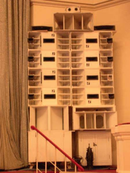
FIGURE 1.34
This loudspeaker escaped from its garage. This is not considered an engineered system (photo courtesy of Dave Lawler).

How do we bridge the gap between the dBV and dB SPL worlds so that we can operate the console in its linear range and ensure that maximum pressure is obtained from the system? The complicating factor here is the presence of transducers in the transmission chain between the electronic and acoustical worlds. Transducers convert energy from one domain to another. Microphones and speakers are our most well-known transducers. They convert acoustical energy to/from mechanical, magnetic and electrical energy, in opposite orders. The domain of mechanical and magnetic energy conversion will be left to the designers and manufacturers of microphones and loudspeakers. We will abridge the matter to an electronic/acoustic transduction, also known as electroacoustic transmission. How much acoustical pressure corresponds to a particular voltage? How much voltage correlates to a particular SPL value?

Sensitivity

One method of expressing this is termed the sensitivity. This parameter bridges the gap by including both expressions. For microphones, the standard sensitivity is given in mV/ pascal. What is a pascal? Ninety-four dB SPL, of course. If a standard SPL level is found at the microphone diaphragm (94 dB SPL), then the voltage at the terminals determines its sensitivity. This is accomplished by a microphone calibration device, known as a pistonphone, which generates a tone and couples to the microphone capsule. For example, the Danish Pro Audio 4007 microphone has a sensitivity of 2.5 mV/Pa. This specification is based only upon the open circuit voltage at the microphone terminals. Because microphones generate both current and voltage, a second sensitivity rating can also be given that factors in the mic's output impedance. This is the “power level” and is specified for a relationship to a standard of 0 dB =1 mW/pascal. Typical microphone power levels run in the −60 to −40 dBV range. Two mics with the same open circuit voltage and different output impedances will have unmatched power level specifications. This complicates our prospects of matching microphones. Fortunately, this is not a concern for us. Since our primary application for microphones is acoustic measurement, we will not be loading down the microphones by splitting them to monitor mix consoles and/or recording trucks. Therefore we will be fortunate to be able to use the far simpler open circuit voltage as our sensitivity specification (Fig. 1.35).

1 watt/1 meter

A full-range loudspeaker sensitivity can be deduced by the inversion of the microphone sensitivity concept. A fixed amount of power is sent to the speaker and the acoustic output is measured. The common representation is 1 watt input drive at 1 meter distance (1W/1m). The SPL generated can then be extrapolated from there provided we know how much power the amplifier is sending. A speaker with a sensitivity of 100 dB (1W/1m) would create 110 dB when driven at 10W and 120 dB with 100 W. This does not mean that it will necessarily generate 130 dB when driven at 1000 W. It may generate smoke instead.

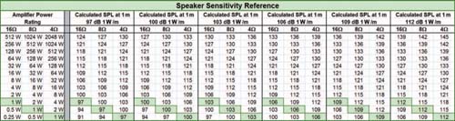
FIGURE 1.35
Speaker sensitivity reference.

A secondary nuisance factor to the sensitivity figure is that it is rated for the standard 1m distance. Other distances must be extrapolated using the inverse square law to determine the SPL at a given location. How much level can this speaker generate at the mix position? Take the sensitivity value and extrapolate that to the maximum rated wattage value, then apply the inverse square law distance loss to the mix position. This provides some insight as to why this figure has limited appeal.

There's more. The 1 W/1m rating fails to factor in the amplifier voltage gain, since it is based on the output power only. This means that speakers driven with different amplifier settings still have matched 1 W/1m values. Things get more complicated for actively biamplified (or triamplified, etc.) speaker systems since 1W will not necessarily appear at the output of both amplifiers simultaneously. Some manufacturers provide separate sensitivity specifications for each driver.

Speaker sensitivity is a holdover from a bygone era. Modern professional audio systems select the power amplifier based on the maximum capabilities of the drivers. The levels are set by how the systems combine acoustically at the acoustic crossover, not by comparing sensitivity values on paper.

Chances are high that we will be listening to an array of speakers, complex mixtures of active multi-way speakers with different drive levels, different amplifiers, and different amounts of acoustic addition over frequency. Again we ask the question: “How many dB SPL can I get out of the console?”

Fortunately, there is a better way.

dB SPL/V

If the amplifier and speaker are viewed as an integrated system, the sensitivity can be viewed in a context relevant to our modern systems with line level console and signalprocessing drive levels. The first question is: “Can the amplifier/speaker system be driven to full power by the drive electronics with a reasonable amount of headroom?” The second question is: “How loud will the system get at a given location in the room when driven at a nominal level?” The answer can be found with a modernized sensitivity value, which denotes the dB SPL value generated by the speaker when driven at line level: dB SPL/V.

How does this work? The electronic transmission components have standard operating level centering around 1 V (0 dBV) and ranging to a maximum of 18–24 dB above that. How many dB SPL will the amplifier/speaker system generate when driven at 1 V? Drive the system at 0 dBV and measure the acoustic level with an SPL meter. Anywhere. With any size or complexity of array. The acoustic gain of the speaker coupling, the equalization, the delay settings, and the amplifier drive levels, even the room, are all included in the data. Add more speakers and it will get louder. The dB SPL/V value will reflect this increase in system capability. Add 20 dB to the dB SPL/V figure and you have the absolute maximum SPL the system can create before the drive electronics clip. This is a measurement we can apply directly to our system.

Before we move on, let's take a brief moment to consider the case of self-powered speakers. The 1 W/1m sensitivity rating is rendered truly academic in a system that has a line level input. The dB SPL/V figure is able to illustrate what the speaker can do with a nominal drive level.

MAXIMUM POWER CAPABILITY

We have seen how we can drive the speakers to their maximum levels. But what are their maximum levels? Power is the scalar factor for speakers. High SPL comes from big (expensive) speakers. Because the scalar factor translates so directly to cost, the power capability decision will be one of the most critical in our design.

The specifications for modern professional speakers go beyond the 1 W/1m sensitivity rating. The maximum levels, for both short duration and long term, are specified. The transient nature of our signal makes both of these important. The specifications are fairly straightforward.

DISTANCE AND ORIENTATION

These specifications are normally given as an axis at a distance of 1m from the speaker. The exceptions to this are loudspeakers that are so large that the 1m distance is too close to characterize the response. The maximum SPL that we can expect to achieve is extrapolated from the maximum SPL data by employing the inverse square law.

dB SPL peak

This is the absolute maximum pressure that the speaker can create. This figure is derived by driving the speaker with an instantaneous burst of pink noise or music. This number does not mean that the speaker can reach this point without distortion, or that it can be sustained for an extended duration. The speaker can reach this level. Period. This specification is relevant to the reproduction of material with high peak content such as drums.

dB SPL continuous

This is the sustainable pressure level over an extended period of time. The time is at least long enough for the system limiters to have engaged. This number should be 6–12 dB lower than the peak. If it is not, then one of three things is likely occurring: the peak limiters are too aggressive, the amplifier is too small and is clipping off the peaks, or the RMS limiters are too loose and the speaker will likely live a short life.

Weighting

Weighting functions are used to tailor the response to mimic the equal loudness contours in the human hearing mechanism. Our hearing is nonlinear, giving us different frequency responses over level. At the low levels, our hearing favors the range centered around the vocal spectrum, which helps us to hear when people are whispering about us. At high levels, our hearing flattens out and then reduces the high and LF extremes. “A” weighting is a filtering added to SPL measurements that mimics the quiet response. “C” weighting mimics the very loud response. “A” weighting has its place in noise floor measurements— not in maximum SPL. “C” weighting has some applicability to high-level measurements. If no weighting is specified, the specification is assumed to be unweighted (linear).

dB SPL will be a key selection criteria for our design process. Different types of program material will require different dB SPL levels to satisfy our expectations. The maximum dB SPL capability of a single speaker unit will be used to classify speakers. Different levels of speakers can be mixed together as long they are traveling proportionally different distances. There are no “heavy metal” speakers. A low-power speaker at a short distance can keep up with a high-power speaker at a long distance.

The relationship between dB SPL, distance, and program material is shown in Fig. 1.36. For a given speaker, its capability to satisfy the power needs falls over distance. Power

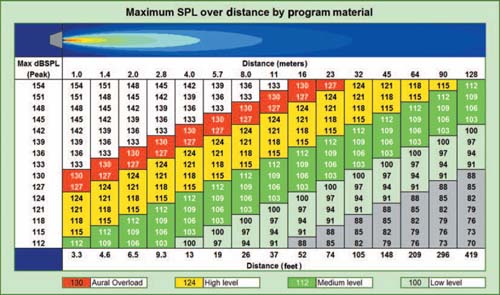
FIGURE 1.36
Typical maximum SPL (peak) over distance by program material.

capability is the most intuitive of all of the speaker parameters. Everyone has their own experiential feeling as to the power needs of a particular genre, and of how well a particular speaker fares in that regard. The figures here should be considered as a reference, but not as definitive. What one of us calls extreme level, others wonder when the show is going to start. We will return to this later when we look at how speakers can sum together to increase SPL.

Half-space loading

Many speaker specifications give their SPL numbers with the speaker measured on the ground. This couples the LF range and raises the SPL number. When comparing models, we need to make sure all speakers were measured under similar conditions.

FREQUENCY RANGE

The frequency range of our transmission was defined earlier as 31 Hz to 18kHz. Professional loudspeaker systems are incapable of spanning this entire range with a single transducer. This is a simple case of “you can't get there from here.” If the tweeter is made big enough to reproduce the lows, it is too heavy to reproduce the highs. If the woofer is made light enough to reproduce the highs, it will fall apart while trying to push out the lows. We bring in specialists to do the work of the different sections of the frequency range. The division generally goes at least three ways: into subwoofer, lows, and highs. Together we have a fullrange system. Note the obvious: the subwoofer is part of the system. It is not a piece of circus equipment that is brought in to provide sonic pyrotechnics. While this may be the case in some applications, this is not the role of a subwoofer in an optimized design. If the subwoofer is intended to provide special effects, it will stand alone as a separate system, and will not be part of the minimum variance transmission strategy. If our intent with the subwoofer is to extend the LF range and SPL capability of the system, then it must be integrated into the system. Our discussion will treat subwoofers and mid-bass systems as range extension and SPL boosters within the main system (Fig. 1.37).

Full-range speakers

The term “full range” connotes a speaker that covers the entire range of the human voice. Most full-range speakers have an LF cutoff range around 60–70 Hz. Larger units with 15″ drivers will reach lower frequencies, while those with 10″ LF drivers or less will roll off closer to 100Hz. The HF range of such devices usually extends up to 18 kHz. Smaller-format speakers with very-low-mass HF drivers will have range extension above the high-power systems, which have heavier diaphragms to accommodate their power requirements. The LF range of these systems will not be required to do the work alone in the bottom end. They may overlap the subwoofers or possibly be crossed over above their LF cutoff and be relieved of LF transmission.

FIGURE 1.37
Overlapping frequency ranges: “full range” + sub, full + mid-bass.

Mid-bass

Mid-bass systems can be used to provide additional SPL capability in the lower mid-range (60–160 Hz). This frequency range has extraordinarily high SPL requirements in the popular music genre. Dedicated mid-bass cabinets may also have improved LF directional control over the full-range systems in the shared range. If the systems are allowed to overlap their frequency ranges, the coverage pattern will be altered by the acoustic summation. Summation will be discussed in detail in Chapter 2. For now, we will note that allowing some degree of overlap is a viable option in this case. Mid-bass systems can also be allowed to have substantial overlap with the subwoofers.

Subwoofers

Subwoofers generally run from 30 to 125 Hz. Subwoofers may overlap with the full-range systems or operate in the LF range alone. If mid-bass systems are used the subwoofers may optionally overlap them.

SPEAKER DIRECTIVITY

In the case of the fireworks explosion discussed previously, the radiation from the source was omnidirectional, i.e., equal pressure was sent in all directions. The upper half of the acoustic power of the explosion was wasted since no audience members were located in the air above the sound source. If the fireworks company were able to invent an explosive device that only radiated below it, they would need only half the acoustic power and the audience would be none the wiser. Black powder is cheap compared to the technology it would take to control the sound, so don't look for much research and development on this front.

This is not the case in sound systems. The potential benefits of controlling speaker directionality make it worthwhile to expend the time and money. The most compelling reason for controlling speaker directionality is the degrading effects of echoes. The sound of fireworks echoing off surfaces further enhances our experience. For our speakers, a little bit of echo goes a long way. Excessive reflections will degrade the intelligibility and modify the tonal content of the music. Prevention begins with controlling the directionality so that minimal energy is sent into spaces where we don't have audience members.

There are two principal mechanisms that create directional control in a loudspeaker system: the interaction of the speaker with a boundary, and the interaction of a speaker with another speaker. Boundary interaction includes horns, walls, wave guides, manifolds, and an assortment of names invented by marketing departments. The shape of the radiating element, such as a cone driver, will also affect the free-field directionality of a single loudspeaker. This is beyond our scope here and the circular cone driver is assumed. Speaker interaction with other speakers can occur both inside of a single enclosure and in separate units.

These two mechanisms share much more than one might expect. The reflected energy from a boundary is essentially a secondary sound source. It will combine with the direct sound in much the same way as will the direct sound of two speakers. This is consistent with the principles of acoustical summation, which will be described in detail in Chapter 2. Directional control is the result of positive phase addition in one direction and cancellation in the other. Cancellation gets a bum rap in our audio society but without it we have very few options for pattern control.

The facility with which directionality is controlled is frequency-dependent or, more precisely, wavelength-dependent. In the case of boundary steering, the length of the boundary must be sufficient compared to the radiated wavelength, to achieve control. As wavelength increases, the boundary must increase proportionally to maintain the same directionality. One quarter wavelength is commonly considered the minimum boundary size to achieve a strong effect. This is easily achieved at high frequencies, but would require a horn that is 2 m deep to control 30 Hz. For lower frequencies, the steering is achieved more practically by using the summation properties of multiple speakers.

Defining the coverage pattern

The directional aspects of loudspeakers are the result of filter effects that operate spatially in the vertical and horizontal planes. The radial shape that this creates around the speaker is the coverage pattern. This is a shape, not a number. A subset of the coverage pattern is the area where the filter effects are less than 6 dB of attenuation. This is the coverage angle. The coverage angle is expressed as a number in degrees (Fig. 1.38).

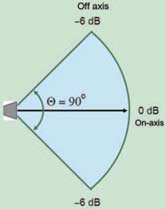
FIGURE 1.38
Coverage angle as found by the radial (protractor) method.

Using the on-axis level of the speaker as a reference, the coverage angle edges are found by moving off-axis in an arc until the response has dropped 6 dB. This is done separately for both the vertical and horizontal planes and for different frequency ranges.

Representations of both coverage pattern and angle have the common feature of normalization to the on-axis response. For the given frequency range the specified values are relative to the on-axis level, no matter what that level is in absolute terms. For example, if the HF horn generates 100 dB SPL @ 1 m on-axis at 1 kHz, the off-axis points are found when the level falls to 94 dB SPL at that same distance. If the frequency is changed to 30 Hz, the polar pattern can still be determined even though the on-axis response might be 60 dB down from the 1 kHz on-axis response, and of no practical value. Coverage renderings only tell us relative level over angle, not indicative of the power capability of the speaker over frequency or of its on-axis frequency response.

Just as we had a variety of methods for expressing voltage in the previous section, so it is for coverage pattern. Coverage patterns are relevant because off-axis sound does not simply cease after the −6 dB point has been exceeded.

Common representations of speaker coverage:

1. Coverage angle: The angle between the equidistant −6 dB points at a given frequency, or range of frequencies. Known as the “radial” or “protractor” method. Specified separately for vertical and horizontal planes.

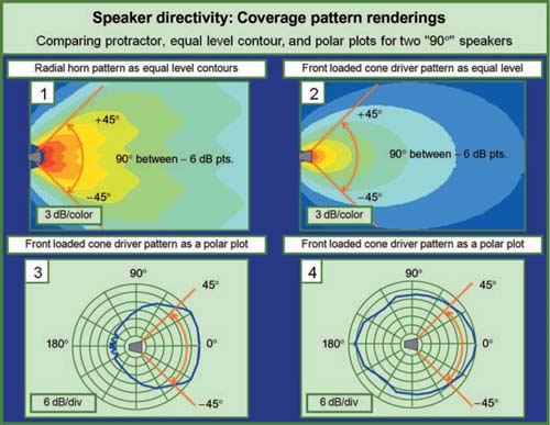
FIGURE 1.39
Equal level contour method of HF (1) and LF drivers (2). Both have 901 coverage angles. Polar plots of the same HF driver (3) and LF drivers (4).

2. Polar pattern: A radial plot of relative level over angle. The data is plotted on a series of concentric rings, which represent relative level loss. The outermost ring is 0 dB loss and the inner rings represent a given number of dB down. The most common formats are 6 and 10 dB per ring. A continuous radial function is created with the values of loss over angle. A pair of typical polar plots is shown in Fig. 1.39. Specified for vertical and horizontal planes over frequency.

3. Equal level contours (isobaric contours): A radial plot of SPL loss over distance from the source. Take a polar plot, turn it inside out, plot it on a linear axis and you have the equal level contour map. The equal level contour map places 0 dB at the 1 m distance from the speaker (the standard measurement point for speaker data). The plot traces the radial shape that maintains the same level. Successive rings show the level drop over distance over angle. Specified for vertical and horizontal planes over frequency (also shown in Fig. 1.39).

4. Directivity index (DI): This parameter describes the directional capability of the system over the entire sphere of radiation. The index compares a given speaker to an idealized omnidirectional reference and therefore a measured omnidirectional speaker has a DI of 0 dB. As directionality increases, the DI value rises as the log of the ratio between the measured and reference. Recall our previous discussion of the fireworks. We have a fixed amount of energy at our source. The DI tells us how much of that energy we are focusing in the forward direction. The term “front to back ratio” is also used to describe this relationship. The DI values are given as a single value for the specified frequency range.

5. Directivity factor (Q): This is a linear version of the DI. The DI value is the 10 log equivalent of the Q factor value. These two values (DI and Q) can be plotted on the same graph with different vertical axis numberings.

6. Beamwidth vs. frequency: Beamwidth is an expression of coverage angle over frequency. Beamwidth plots create a composite of the full frequency range of the speaker from a series of individual coverage angles. Resolution is typically octave or one-third octave, allowing us to view the speaker's coverage angle trends in a single chart. Since the beamwidth is made up of coverage angle values, the off-axis response is not included. See Fig. 1.40.

90 degrees of separation

Each of these coverage representations tells us about our speakers. Do we need to factor all of them in to making our decisions? This myriad of coverage data can be overwhelming to those of us that just want to figure out what is the best speaker and where to point it, within our short life span. Which of these representations is most relevant to our task? We will cover this in more detail later in Section 2, but for now let's present them all with a simple task and see how they fare. The test will be to determine the speaker coverage angle required for the most uniform level over four different shapes. Let the games begin.

FIGURE 1.40
Beamwidth vs. frequency of a small-format full-range loudspeaker. Coverage angle is 90° (nominal).

Figure 1.41 shows a section view with four vertical coverage lines labeled A through D. The same speaker location is used for all shapes. From the speaker's perspective, the angle between the first and last seat is unchanged in all cases. It is the distance relative to the

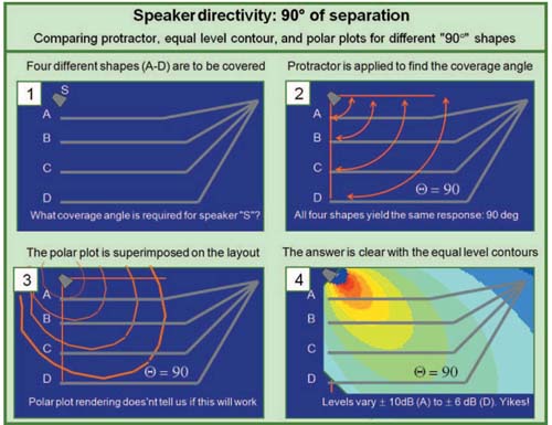
FIGURE 1.41
Four shapes are shown for coverage from a single speaker location. (1) Listening location targets A–D. The speaker is closest to shape A and farthest from shape D. (2) Protractor method indicates the application requires 90° of coverage in all cases since the angle between the first and last seat is constant. (3) The polar plot shape using 90° coverage plots provides no clear linkage to the listening area shapes. (4) Equal level contours method shows the level uniformity to be poor in all cases, and worst for shape A.

lower part of the shape that changes in each case. The first question is: what is the required coverage angle? The answer is found in panel 2. It is 90° in all cases, since we will cover from the top rear to the front near. The differing distance to the floor does not change the angular relationship from the speaker to either the top or bottom extremes. It does, however, introduce a gross asymmetry between the distances to the respective coverage edges. The asymmetry is highest for shape A and lowest for shape D. This is the principal vulnerability of the radial(protractor) method.

Panel 3 employs the polar plot to attempt to discern the best angle. Unfortunately the polar plot gives us no further insight beyond seeing the off-axis shape of the speaker. The vulnerability of the polar plot is that its rendering of level does not scale to the room geometry. In the room pictogram we can assume that a doubling of distance from the source will equate to a loss of approximately 6 dB. In the polar plot, the 6 dB lines are evenly spaced, which would be analogous in the room to 6 dB loss per meter, rather than per doubling (refer back to Fig. 1.39). Therefore we cannot overlay the polar plot on the room pictogram and ascertain the level distribution in any of the shapes. All we know is that at 45° off-axis we are down 6 dB, a fact we already hand in hand from the protractor. Is it 6 dB down in the backseats? In the front? I have no idea. Next we apply the equal level contour method. Panel 4 shows the 90° contours with the 45° down tilt that would center the speaker over the complete coverage angle. In all cases (A–D), the entire seating area is within the coverage angle of the speaker. In all cases, the people in the rear of the listening area are more than 8 dB down from the front. This is obviously a very unsatisfactory result. The good news is we have proven that this aim angle won't work, so now we can embark on finding out what will work. The equal contour method gives us clues to find the angles that will best serve the four different shapes.

There is no figure/pictogram for the DI or directivity factor (Q) methods. What would those methods be? With a single number that

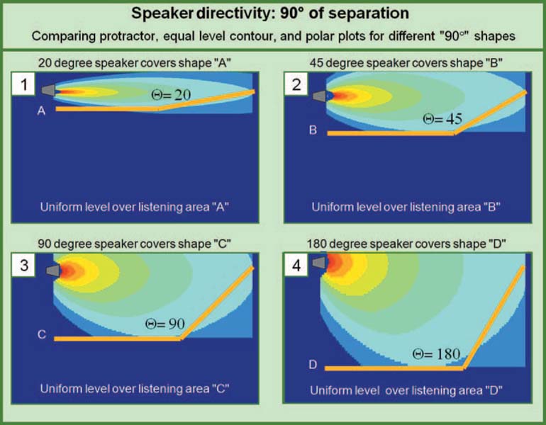
FIGURE 1.42
Equal level contours method using four different coverage angles. The shape of the contours reveals the best fit for each room.

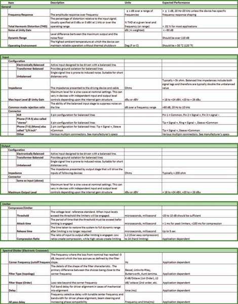
FIGURE 1.43
Universal Generic Specification Sheet.

FIGURE 1.43 (Continued).

comprises vertical and horizontal directivity we don't have much to work with. If the front/back ratio is positive (DI>0 dB, Q>1), then we know to point the front side toward the audience. This is a start but we will need to be a bit more specific. Do we need a 90 × 40 speaker? How can we tell? If we somehow decided on a 90×40, the DI value would it be the same whether we oriented it in the horizontal or the vertical plane. I would think we need to know that. The answer lies in four different speaker coverage patterns applied to the four different audience shapes. In all cases, the speaker is oriented asymmetrically—at the farthest seat, in order to compensate for the asymmetry of the space. The equal level contours are the best indicator of how well we compensate for asymmetry, since they indicate level directly. Since many coverage applications are asymmetrical, this is a critical parameter. Figure 1.42 utilizes the equal level contour method to find the best fit for each shape. Each color gradient represents 3 dB of level change. In each case, a different coverage angle is found, as determined by the coverage pattern. The determining factor is the coverage pattern shape that most closely follows the line of coverage. (1) The asymmetry between the on-axis and off-axis distance is at its maximum. The coverage angle (20°) is the smallest. (2) The distance and orientation to the rear remains the same but the level to the floor is increased. The increased distance down to the floor decreases the asymmetry. Less asymmetry yields to wider coverage of 45°. (3) Coverage angle opens to 90°. Note that while the 90° angle is equal to that of the radial coverage angle method, the orientation of the spe0aker is different. (4) Coverage reaches maximum symmetry. Coverage widens to 180°.

The equal level contours lead us toward selection of both coverage angle and orientation, even when faced with an asymmetrical coverage situation. Asymmetry will be a pivotal issue in our designs, e.g., every vertical coverage application for starters. Our analysis of coverage angle will need to be able to deal with asymmetry.

Naturally, we are concerned about having the upper half of the pattern bouncing off of the walls. At first glance, this approach would be a cause of great concern in this regard, perhaps even a lapse of sanity on my part. Take a breath. Bear in mind that we are discussing the behavior of a single speaker. This is the building block, not the finished product. The optimal solutions for creating asymmetric coverage patterns will come from arrays of speakers. The behavior of speaker arrays is the summation of its individual speaker parts. Before we learn to run, we will first need to walk.

Specifications

We have now introduced the components of the sound system. We have many choices in the marketplace so we need to be conversant in the language used to specify the performance of the products. Each device has both unique and common characteristics, and these in turn may be described in unique or common terminologies. This section is intended to serve as a reference aid in the navigation through manufacturer's spec sheets so that we can ensure that our choices will be suitable for a well-optimized system. This discussion will be short as we will let the reference chart in Fig. 1.43 do the talking for us. The list is by no means comprehensive but will be sufficient to head us in a forward direction. The chart contains a list of the principal features of the components and a brief description. The relevant parameters are shown and expected results indicated. The last column, where applicable, links the tested parameter to test instruments and procedures described in the later chapters of this book.

SUMMARY

■ The goal of transmission is to accurately transport the original waveform through different devices, over different media and over distance.

■ An audio waveform is made up of individual sine waves with independent amplitude and phase characteristics.

■ Analog audio transmission requires a medium.

■ The relationship of time and frequency is reciprocal and medium-independent.

■ The size of the wavelength increases with the transmission speed and decreases with frequency.

■ The speed of sound in air varies over temperature.

■ Waveforms with different frequency content mix together, while those with common content sum together.

■ The magnitude variations of audio waveforms are so large that they are quantified on a log scale (dB).

■ dB levels can be scaled relative to a fixed or relative standard.

■ Polarity is a term to describe the orientation of the transmitted waveform to its original form. It is either identical (normal, non-inverting) or reversed.

■ The minimum time required to transmit through a medium is known as the “latency.”

■ Transmission power is a combination of voltage and current (electrical) or pressure and surface area (acoustic).

■ Transmission can be variable in level or time over frequency. Such differences are called the “frequency response.”

■ The stated range of human hearing is 20 Hz to 20 kHz but the practical range of transmission is 30 Hz to 18 kHz, a ratio of 600×.

■ Line level devices have a nominal range of 1 V (0 dBV) and maximum level of 20 V. (+26 dBV).

■ Noise is minimized in the interconnection between line level devices by use of balanced lines.

■ Typical line level devices use low-impedance outputs to drive high-impedance inputs.

■ Digital transmission has no media, instead transporting the waveform as a mathematical rendering.

■ Acoustic transmission is typically quantified in pressure at a point in space: dB SPL.

■ Loudspeakers are characterized primarily by their maximum SPL, their frequency range, and coverage angle.

■ There are many different methods of characterizing the coverage angle. The equal level contours method shows the lines of uniformity over the space.

REFERENCE

Giddings, P. (1990). Audio system: Design and installation.Sams.