
4.3 Binaural Cue Coding (BCC)
4.3.1 Time–frequency processing
BCC processes audio signals with a certain time and frequency resolution. The frequency resolution used is largely motivated by the frequency resolution of the auditory system (see Chapter 3). Psychoacoustics suggest that spatial perception is most likely based on a critical band representation of the acoustic input signal [26]. This frequency resolution is considered by using an invertible filterbank with sub-bands with bandwidths equal or proportional to the critical bandwidth of the auditory system [98, 293]. The specific time and frequency resolution used for BCC is discussed later in Section 4.3.3.
4.3.2 Down-mixing to one channel
It is important that the transmitted down-mix signal contains all signal components of the input audio signal. The goal is that each signal component is fully maintained. Simple summation of the audio input channels often results in amplification or attenuation of signal components. In other words, the power of signal components in the ‘simple’ sum is often larger or smaller than the sum of the power of the corresponding signal component of each channel. Therefore, a down-mixing technique is used which equalizes the down-mix signal such that the power of signal components in the down-mix signal is approximately the same as the corresponding power in all input channels.
Figure 4.2 shows the down-mixing scheme. The input audio channels xc(n) (1 ≤ c ≤ C) are decomposed into a number of sub-bands. One such sub-band is denoted ![]() c(k) (note that for notational simplicity no sub-band index is used). Since similar processing is independently applied to all sub-bands it is sufficient to describe the processing carried out for one single sub-band. A different time index k is used since usually the sub-band signals are downsampled.
c(k) (note that for notational simplicity no sub-band index is used). Since similar processing is independently applied to all sub-bands it is sufficient to describe the processing carried out for one single sub-band. A different time index k is used since usually the sub-band signals are downsampled.
The signals of each sub-band of each input channel are added and then multiplied by a factor e(k)
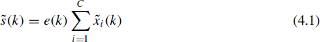
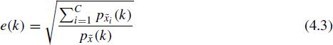
The factor e(k) is computed such that
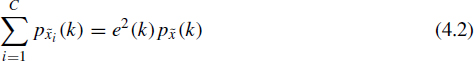
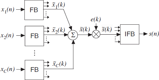
Figure 4.2 The down-mix signal is generated by adding the input channels in a sub-band domain and multiplying the down-mix with a factor in order to preserve signal power. FB denotes filterbank and IFB inverse filterbank. The processing shown is applied independently to each sub-band.
where p![]() i(k) is a short-time estimate of the power of
i(k) is a short-time estimate of the power of ![]() i(k) at time index k and p
i(k) at time index k and p![]() (k) is a short-time estimate of the power of ΣCi=1
(k) is a short-time estimate of the power of ΣCi=1![]() i(k) From (4.2) it follows that
i(k) From (4.2) it follows that
The equalized sub-bands are transformed back to the time domain, resulting in the down-mix signal s(n) that is transmitted to the BCC decoder.
An example for the effect of the described down-mixing with equalization is illustrated in Figure 4.3. The top two rows show two signals and their respective magnitude spectra. The bottom row shows the sum of the two signals and the magnitude spectra of the ‘simple’ sum signal and the equalized sum signal as generated with the scheme shown in Figure 4.2. In the range from 500 Hz to about 1 kHz the equalization for this example prevents that the sum signal is significantly attenuated. The top panel in Figure 4.4 shows the same data as shown in the bottom right panel in Figure 4.3. The bottom panel of Figure 4.4 shows the normalized magnitude spectra for down-mix (thin) and equalized down-mix (bold). At each frequency the normalization is relative to the total (sum of) input signal channel power. As desired, with equalization, the normalized magnitude spectrum is 0 dB.
These examples are somewhat artificial since the x1 and x2 signals look more like impulse responses (direct sound plus one reflection) than real-world signals. Equalization can be understood as modifying the interactions of impulse responses to prevent attenuation or amplification of signal components due to certain phase interactions.
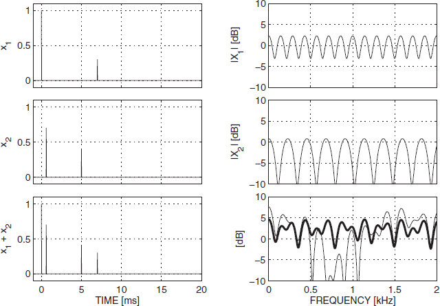
Figure 4.3 Two signals x1(n) and x2(n) and their respective magnitude spectra X1(f) and X2(f) (top two rows). Down-mix signal x1(n) + x2(n) magnitude spectrum (bottom right, thin) and equalized down-mix signal magnitude spectrum (bottom right, bold) are shown.
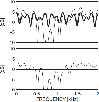
Figure 4.4 Top: down-mix signal x1(n) + x2(n) magnitude spectrum (thin) and equalized down-mix signal magnitude spectrum (bold). Bottom: normalized down-mix signal magnitude spectrum (thin) and normalized equalized down-mix signal magnitude spectrum (bold).
4.3.3 ‘Perceptually relevant differences’ between audio channels
The basic operation principle of BCC is to reconstruct a stereo or multi-channel audio signal from the mono down-mix signal that sounds virtually identical to the original stereo or multi-channel content, by reinstating perceptually relevant spatial properties. In Chapter 3 it is explained that in the horizontal plane, ICLD, ICTD and ICC parameters are the most relevant attributes that determine the perceived spatial image. The ICLD and ICTD parameters are associated with the perceived position of a sound source, while the ICC corresponds to a perceived ‘width’ of one sound source (for example introduced by reflections in a room), and it can indicate unreliable ICLD and ICTD parameters if concurrent sources from different directions are present in the same time/frequency region. In the latter case, the ICLD and ICTD parameters will be time and frequency dependent and follow from interactions of the parameters from each sound source individually (a detailed analysis of ICLD, ICTD and ICC parameters for multiple simultaneous sound sources is given in Chapter 8). But besides reflections or concurrent sound sources, low ICC values may also result from certain effects applied by audio engineers.
The human auditory system has access to ICLD, ICTD and ICC parameters, but its accuracy to analyze these cues is limited. The first limitation exists in the temporal domain. As described in Chapter 3, fast variations of binaural cues can not be tracked by the human auditory system. This behavior seems best described by analysis of a certain ‘window’ with a typical length of 30–60 ms from which the ICLD, ICTD and ICC parameters are estimated. An important consequence of such an integration window is that very fast variations in either ICLD or ICTD (i.e., variations within one analysis window) result in a decrease of the ICC that is estimated from that window. In other words, fast variations in ICTD and ICLD can be detected, but are perceived as a change in the width rather than fast movements and consequently cannot be tracked in terms of position. Contrary to such an window-averaging model, in precedence-effect situations, the perceived spatial attributes are dominated by the first few milliseconds of a signal onset, ignoring spatial attributes of a significant portion of the remainder of the signal.
A second limitation that was explained in Chapter 3 is the limited frequency resolution to analyze binaural cues. Specifically, on top of the temporal resolution limitations described above, binaural cues seem to be rendered in critical bands only. Moreover, given the finite slope of the so-called auditory filters, significant correlation between binaural cues from adjacent filters is expected, which may loosen the spectral design criteria for BCC schemes somewhat.
A third limitation that can be exploited in BCC is the fact that binaural cues require a certain minimum change in order to be perceived. This property forms the basis for a limited repertoire of binaural cue values, which are closely matched to just-noticeable differences in each cue.
In the current description, filterbanks with sub-bands of bandwidths equal to two times the equivalent rectangular bandwidth (ERB) [98] are used. Informal listening revealed that the audio quality of BCC did not notably improve when choosing higher frequency resolution. A lower frequency resolution is favorable since it results in less ICTD, ICLD, and ICC values that need to be transmitted to the decoder and thus in a lower bitrate.
Regarding time-resolution, ICTD, ICLD, and ICC are considered at regular time intervals of about 4–16 ms. Note that using such intervals, the precedence effect is not directly considered. Assuming a classical lead–lag pair of sound stimuli, when the lead and lag fall into a time interval where only one set of cues is synthesized, localization dominance of the lead is not accounted for. Despite this, BCC achieves audio quality reflected in an average MUSHRA score [148] of about 87 (‘excellent’ audio quality) on average and up to nearly 100 for certain audio signals [12]. Hence when using a fixed update rate of about 4–16 ms, a good trade-off between bit rate and quality is obtained. A dynamic, signal-dependent segmentation process can further improve the performance (see Chapter 5) by lowering the average update rate while at the same time providing a high temporal resolution at signal onsets to account for the precedence effect.
The often achieved perceptually small difference between reference signal and synthesized signal implies that cues related to a wide range of auditory spatial image attributes are implicitly considered by synthesizing ICTD, ICLD, and ICC at regular time intervals. In the following, some arguments are given on how ICTD, ICLD, and ICC may relate to a range of auditory spatial image attributes.
Source localization (auditory object direction)
The model for source localization described in Section 3.6 speculates about a possibly important role IC may play for source localization. This includes localization of sources in the presence of concurrent sound and reflections. The validity of this model would in many cases justify the use of ICTD, ICLD, and ICC only at regular time intervals without explicitly considering the precedence effect for real-world audio signals.
Attributes related to reflections
Early reflections up to about 20 ms result in coloration of sources' signals. This coloration effect is different for each audio channel determined by the timing of the early reflections contained in the channel. BCC does not attempt to retrieve the corresponding early reflected sound for each audio channel (which is a source separation problem). However, frequency dependent ICLD synthesis imposes on each output channel the spectral envelope of the original audio signal and thus is able to mimic coloration effects caused by early reflections.
Most perceptual phenomena related to spatial impression seem to be related directly to the nature of reflections that occur following the direct sound. This includes the nature of early reflections up to 80 ms and late reflections beyond 80 ms. Thus it is crucial that the effect of these reflections is mimicked by the synthesized signal.
ICTD and ICLD synthesis ideally result in that each channel of the synthesized output signal has the same temporal and spectral envelope as the original signal. This includes the decay of reverberation (the sum of all reflections is preserved in the transmitted sum signal and ICLD synthesis imposes the desired decay for each audio channel individually). ICC synthesis de-correlates signal components that were originally de-correlated by lateral reflections. Also, there is no need to consider reverberation time explicitly. Blindly synthesizing ICC at each time instant to approximate ICC of the original signal has the desired effect of mimicking different reverberation times, since ICLD synthesis imposes the desired rate of decay.
The most important cues for auditory object distance are overall sound level and direct sound to total reflected sound ratio [238]. Since BCC generates level information and reverberation such that it approaches that of the original signal, auditory object distance cues are represented by considering ICTD, ICLD, and ICC cues.
4.3.4 Estimation of spatial cues
In the following, it is described how ICTD, ICLD, and ICC are estimated. (Depending on the transform that is used to enable sub-band processing, it is sometimes more convenient to analyze inter-channel phase differences (ICPDs) instead of ICTDs, which will be outlined in Chapter 5.) The bitrate required for transmission of these spatial cues is just a few kb/s and thus with BCC it is possible to transmit stereo and multi-channel audio signals at bitrates close to what is required for a single audio channel.
Estimation of ICTD, ICLD, and ICC for stereo signals
The scheme for estimation of ICTD, ICLD, and ICC is shown in Figure 4.5. The following measures are used for ICTD, ICLD, and ICC for corresponding sub-band signals ![]() 1(k) and
1(k) and ![]() 2(k) of two audio channels:
2(k) of two audio channels:
ICTD [samples]:
![]()
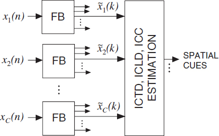
Figure 4.5 The spatial cues, ICTD, ICLD, and ICC are estimated in a sub-band domain. The spatial cue estimation is applied independently to each sub-band.
with a short-time estimate of the normalized cross-correlation function
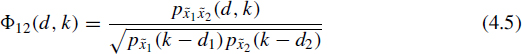
where
and p![]() 1
1![]() 2(d, k) is a short-time estimate of the mean of
2(d, k) is a short-time estimate of the mean of ![]() 1(k − d1)
1(k − d1) ![]() 2(k − d2).
2(k − d2).
ICLD [dB]:
ICC:
![]()
Note that the absolute value of the normalized cross-correlation is considered and c12(k) has a range of [0, 1]. Out-of-phase signal pairs can not be represented by these cues as defined. Real-world audio signals only contain phase-inverted signal components in unusual cases and are not explicitly considered here. An alternative ICC/ICTD representation that does allow for out-of-phase signal pairs is outlined in Chapter 6.
Estimation of ICTD, ICLD, and ICC for multi-channel audio signals
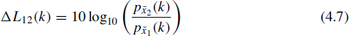
The estimation of inter-channel cues between more than 2 channels is somewhat more complex than for the two-channel case as explained above. In principle, C(C − 1) pairs exist to compute parameters from. Due to symmetries in the parameter definition, this will result in C(C − 1)/2 unique parameter values (see Figure 4.7(a) for a five-channel example). For the ICLD, all channel levels are uniquely defined by C − 1 ICLD parameters given inter-relations of ICLD parameters and the fact that the overall power should be preserved with respect to the down-mix. For example, in a three-channel case, the ICLD between channel 2 and 3 is fully determined by the ICLDs between channel 1 and 2 on the one hand, and channel 1 and 3 on the other hand. For ICTD and ICC, however, such relations between pair-wise parameters do not exist. However, it was nevertheless found that for the ICTD,C − 1 parameters seem sufficient to obtain a perceptually correct spatial image. The ICTD (and ICLD) parameters are defined against one single reference channel. This is illustrated in Figure 4.6 for the case of C = 5 channels. τ1c(k) and ΔL1c(k) denote the ICTD and ICLD between the reference channel 1 and channel c.
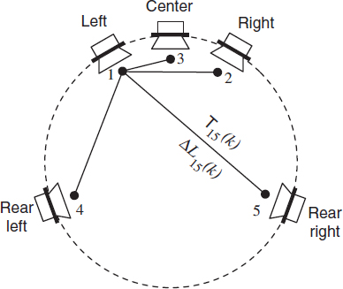
Figure 4.6 ICTD and ICLD are defined between the reference channel 1 and each of the other C − 1 channels.
For ICC, a different approach is used. As opposed to using the ICC between all possible channel pairs, it has shown to be sufficient to consider just a few or even a single ICC parameter to indicate the overall coherence or ‘diffuseness’ of the audio channels. One possibility is to estimate and transmit only ICC cues between the two channels with most energy in each sub-band at each time index. This is illustrated in Figure 4.7(b), when for time instants k − 1 and k the channel pairs (3, 4) and (1, 2) are strongest, respectively. The decoder uses this ICC value to determine its de-correlation processing. A different method of reducing the number of ICC parameters is used in MPEG Surround by employing a tree structure of pair-wise channel comparisons as outlined in Chapter 6.
4.3.5 Synthesis of spatial cues
Figure 4.8 shows the scheme which is used in the BCC decoder to generate a stereo or multi-channel audio signal, given the transmitted sum signal plus the spatial cues. The sum signals(n) is decomposed into sub-bands, where ![]() (k) denotes one such sub-band. For generating the corresponding sub-bands of each of the output channels, delays dc, scale factors ac, and filters hc are applied to the corresponding sub-band of the sum signal. (For simplicity of notation, the time index k is ignored in the delays, scale factors, and filters).
(k) denotes one such sub-band. For generating the corresponding sub-bands of each of the output channels, delays dc, scale factors ac, and filters hc are applied to the corresponding sub-band of the sum signal. (For simplicity of notation, the time index k is ignored in the delays, scale factors, and filters).
Figure 4.7 Computation of ICC for multi-channel audio signals. (a) In the most general case, ICCs are considered for each sub-band between each possible channel pair; (b) BCC considers for each sub-band at each time instant k, the ICC between the channel pair with the most power in the sub-band considered. In the example shown the channel pair is (3, 4) at time instant k − 1 and (1, 2) at time instant k.
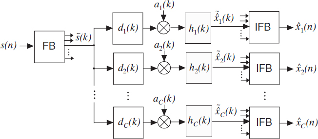
Figure 4.8 ICTD are synthesized by imposing delays, ICLD by scaling, and ICC by applying de-correlation filters. The processing shown is applied independently to each sub-band.
ICTD synthesis
The delays are determined by the ICTDs

The delay for the reference channel, d1, is computed such that the maximum magnitude of the delays dc is minimized. The less the sub-band signals are modified, the less danger there is for artifacts to occur. If the sub-band sampling rate does not provide high enough time-resolution for ICTD synthesis, delays can be imposed more precisely by using suitable allpass filters.
ICLD synthesis
In order that the output sub-band signals have desired ICLDs (Equation 4.7) between channel c and the reference channel 1, ΔL1c(k), the gain factors ac must satisfy
![]()
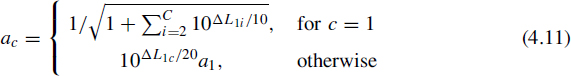
Additionally, the output sub-bands are normalized such that the sum of the power of all output channels is equal to the power of the input sum signal. Since the total original signal power in each sub-band is preserved in the sum signal (Section 4.3.2), this normalization results in that the absolute sub-band power for each output channel approximates the corresponding power of the original encoder input audio signal. Given these constraints, the scale factors are
ICC synthesis
The aim is to reduce correlation between the sub-bands after delays and scaling have been applied, without affecting ICTD and ICLD. Generally speaking, this can be achieved by applying filters, hc in Figure 4.8, in a similar spirit as to generate a certain amount of late reververation. One point of view for designing the filters hc in Figure 4.8 is to vary ICTD and ICLD as a function of frequency such that the average value is zero in each sub-band (i.e., the mean cue within one critical band remains unchanged). Figure 4.9 illustrates how ICTD and ICLD are varied within a sub-band as a function of frequency. The amplitude of ICTD and ICLD variation determines the degree of de-correlation and is controlled as a function of ICC. Note that ICTD are varied smoothly while ICLD are varied randomly. One could vary ICLD as smoothly as ICTD, but this would result in more coloration of the resulting audio signals. Detailed processing for ICTD and ICLD variation as a function of ICC is described in [83].
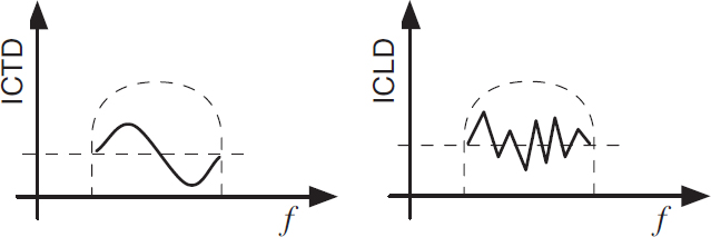
Figure 4.9 ICC is synthesized in sub-bands by varying ICTD and ICLD as a function of frequency.
Another method for synthesizing ICC, particularly suitable for multi-channel ICC synthesis, is described in [82, 218, 233–235]. As a function of time and frequency, specific amounts of artificial (late) reverberation is added to each of the output channels for achieving a desired ICC. Additionally, spectral modification is applied such that the spectral envelope of the resulting signal approaches the spectral envelope of the original audio signal.