
10.3 Spatial decomposition of stereo signals
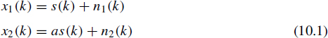
Stereo signals are recorded or mixed such that for each source the signal goes coherently into the left and right signal channel with specific directional cues (level difference, time difference) and reflected/reverberated independent signals go into the channels determining auditory object width and listener envelopment cues. This motivates modeling single source stereo signals, as illustrated in Figure 10.1, where the signal s mimics the direct sound from a direction determined by the factor a. The independent signals, n1 and n2, correspond to the lateral reflections. These signals are assumed to have the following relation with the stereo signal pair x1, x2:
In order to get a decomposition which is not only effective in a one auditory object scenario, but nonstationary scenarios with multiple concurrently active sources, the described decomposition is carried out independently in a number of frequency bands and adaptively in time:
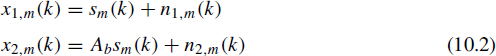
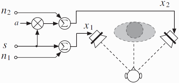
Figure 10.1 Mixing a stereo signal mimicking direct sound s and lateral reflections n1 and n2. The factor A determines the direction at which the auditory object appears.
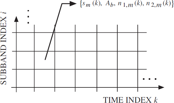
Figure 10.2 Each left and right time–frequency tile of the stereo signal, x1 and x2, is decomposed into three signals, s, n1, and n2, and a factor A.
where m is the sub-band index, k is the time index, and Ab the amplitude factor for signal sm for a certain parameter band b that may comprise one or more sub-bands of the sub-band signals (see also Chapter 5 for more details on sub-bands and parameter bands). The decomposition in separate time/frequency tiles is illustrated in Figure 10.2, i.e. in each time–frequency tile with indices m and k, the signals sm, n1,m, n2,m, and factor Ab are estimated independently. For brevity of notation, the sub-band and time indices are often ignored in the following. Similarly as BCC or MPEG Surround a perceptually motivated sub-band decomposition is used. This decomposition may be based on the fast fourier transform, quadrature mirror filterbank, or other filterbank. For each parameter band, the signals sm, n1,m, n2,m, and Ab are estimated based on segments with a length of approximately 20 ms.
Given the stereo sub-band signal pair, x1,m and x2,m, the goal is to estimate sm, Ab, n1,m, and n2,m in each parameter band. This is performed by analysis of the powers and cross-correlation of the stereo signal pair. A short-time estimate of the power of x1,m in parameter band b is denoted px1,b and is obtained as outlined in Chapter 6, Section 6.3.4. The powers of n1,m and n2,m in each parameter band are assumed to be the same, i.e. it is assumed that the amount of lateral independent sound is the same for the left and right signals:
![]()
10.3.1 Estimating ps,b, Ab and pn,b
Given the sub-band representation of the stereo signal, the power (px1,b, px2,b) and the normalized cross-correlation ρx1x2,b for parameter band b are computed (see also Section 6.3.4). Ab,ps,b, and pn,b are subsequently estimated as a function of the estimated px1,b, px2,b, and ρx1x2,b. Three equations relating the known and unknown variables are:
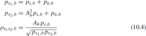
These equations solved for Ab, ps,b, and pn,b, yield
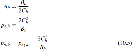
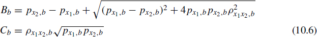
with
10.3.2 Least-squares estimation of sm, n1,m and n2,m
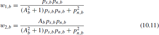
Next, the least-squares estimates of sm, n1,m, and n2,m are computed as a function of Ab, ps,b, and pn,b. For each parameter band b and each independent signal frame, the signal sm is estimated as

where w1,b and w2,b are real-valued weights. The estimation error is
![]()
The weights w1,b and w2,b are optimal in a least mean-square sense when the error signal E is orthogonal to x1,m and x2,m in parameter band b [117], i.e.
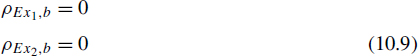
yielding two equations:

from which the weights are computed:
Similarly, n1,m and n2,m are estimated. The estimate of n1,m is

The estimation error is
![]()
Again, the weights are computed such that the estimation error is orthogonal to x1,m and x2,m, resulting in
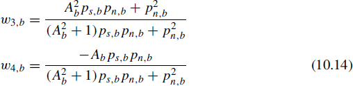
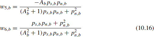
The weights for computing the least-squares estimate of n2,m

10.3.3 Post-scaling
Given the initial least-squares estimates ŝm,![]() 1,m, and
1,m, and ![]() 2,m, post-scaling is applied such that the power of the estimates ŝm,
2,m, post-scaling is applied such that the power of the estimates ŝm,![]() 1,m, and
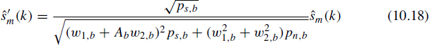
1,m, and ![]() 2,m in each parameter band equals to ps,b and pn,b. The power of ŝm in parameter band b is
2,m in each parameter band equals to ps,b and pn,b. The power of ŝm in parameter band b is
![]()
Thus, for obtaining an estimate of ŝm with power ps,b,ŝm is scaled
With similar reasoning, ![]() 1,m and
1,m and ![]() 2,m are scaled, i.e.
2,m are scaled, i.e.
10.3.4 Numerical examples
The factor Ab (top panel), the ratio ps,b/px1,b (middle panel) and A2ps,b/px2,b (lower b panel) expressed in dB are shown in Figure 10.3 as a function of the stereo level difference px2,b/px1,b (in dB) and the cross correlation ρx1x2,b.
The weights w1,b and w2,b for computing the least-squares estimate of sm are shown in the top two panels of Figure 10.4 as a function of the stereo signal level difference and ρx1x2,b. The post-scaling factor for ŝm (10.18) is shown in the bottom panel.
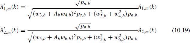
The weights w3,b and w4,b for computing the least-squares estimate of n1,m and the corresponding post-scaling factor (10.19) are shown in Figure 10.5 as a function of the stereo signal level difference and ρx1x2,b.
The weights w5,b and w6,b for computing the least-squares estimate of n2,m and the corresponding post-scaling factor (10.19) are shown in Figure 10.6 as a function of the stereo signal level difference and ρx1x2,b.
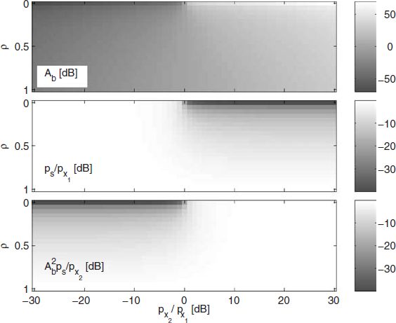
Figure 10.3 The factor Ab (top panel), the ratio ps,b/px1,b (middle panel) and A2ps,b/px2,b (lower panel) expressed in dB as a function of the stereo level difference px2,b/px1,b (in dB) and the cross correlation ρx1x2,b.
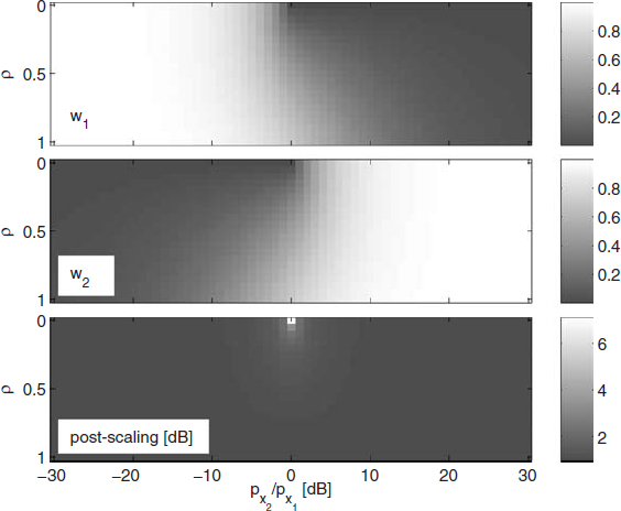
Figure 10.4 The least-squares estimate weights w1,b and w2,b and the post-scaling factor for computation of the estimate of sm.
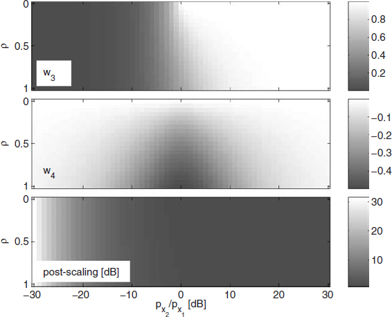
Figure 10.5 The least-squares estimate weights w3,b and w4,b and the post-scaling factor for computation of the estimate of n1,m.
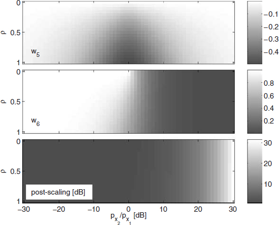
Figure 10.6 The least-squares estimate weights w5,b and w6,b and the post-scaling factor for computation of the estimate of n2,m.
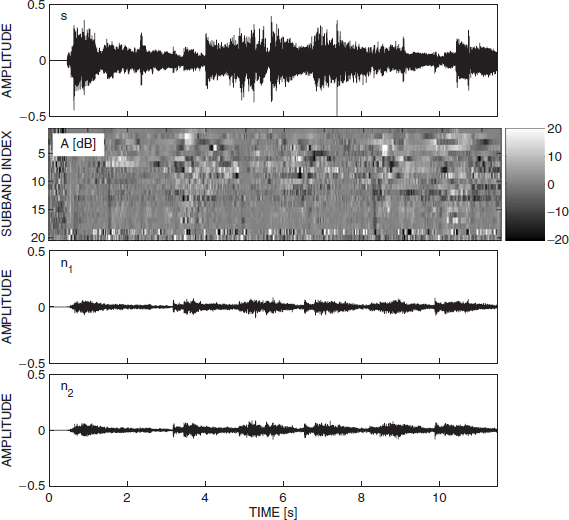
Figure 10.7 Estimates ŝ, Ab, ![]() 1, and
1, and ![]() 2 are shown as a function of time for a short audio clip. The factor Ab is shown for various parameter bands.
2 are shown as a function of time for a short audio clip. The factor Ab is shown for various parameter bands.
An example for the spatial decomposition of a stereo rock music clip with a singer in the center is shown in Figure 10.7. The estimates of s, A, n1, and n2 are shown. The signals are shown in the time domain (i.e. after independent processing of each parameter band and subsequently transforming the signals to the time domain) and Ab is shown for every time-frequency tile. The estimated direct sound s is relatively strong compared to the independent lateral sound n1 and n2 since the singer in the center is dominant.