9. Testing Differences Between Means: Further Issues

There are several ways to test the likelihood that the difference between two group means is due to chance, and not all of them involve a t-test. Even limiting the scope to a t-test, three general approaches are available to you in Excel:

• The T.DIST() and T.INV() functions

• The T.TEST() function

• The Data Analysis add-in

This chapter illustrates each of these approaches. You’ll want to know about the T.TEST() function because it’s so quick (if not broadly informative). You might decide never to use the T.DIST() and T.INV() functions directly, but you should know how to use them because they can show you step by step what’s going on in the t-test. And you’ll want to know how to use the Data Analysis t-test tool because it’s more informative than T.TEST() and quicker to set up than T.DIST() and T.INV().

Using Excel’s T.DIST() and T.INV() Functions to Test Hypotheses

The Excel 2010 worksheet functions that apply to the t-distribution are dramatically different from those in Excel 2007 and earlier. The differences have to do primarily with whether you assign alpha to the left tail of the t-distribution, the right tail, or both. Recall from Chapter 8, “Testing Differences Between Means: The Basics,” that alpha, the probability of rejecting a true null hypothesis, is entirely under your control. (Beta, the probability of rejecting a true alternative hypothesis, is not fully under your control because it depends in part on the population mean if the alternative hypothesis is true—again, see Chapter 8 for more on that matter.)

As I structured the examples in Chapter 8, you suspected at the outset that the mean age of your sample of turtles from the Gulf of Mexico would be less than a hypothesized value of 55 years. You put the entire alpha into the left tail of the curve on the right (see, for example, Figure 8.7). When you adopt this approach, you reject the possibility that the alternative could exist at the other end of the null distribution.

In that example, by placing all the error probability into the left tail of the null distribution, you assumed that Gulf turtles are not on average older than the total population of turtles: Their mean is either smaller than (the alternative hypothesis) or not reliably different from (the null hypothesis) the mean of the total population. This is called a one-tailed or a directional hypothesis.

On the other hand, when you make a two-tailed or nondirectional hypothesis, your alternative hypothesis does not specify whether one group’s mean will be larger or smaller than that of the other group. The null hypothesis is the same, no difference in the population means, but the alternative hypothesis is something such as “The population mean for the experimental group is different from the population mean for the control group”—“different from” rather than “less than” or “greater than.”

The difference between directional and nondirectional hypotheses might seem picayune, but it makes a major difference to the statistical power of your t-tests.

Making Directional and Nondirectional Hypotheses

The main benefit to making a directional hypothesis, as the example in Chapter 8 did, is that doing so increases the power of the statistical test. But there is also a responsibility you assume when you make a directional hypothesis.

Suppose that, just as in Chapter 8, you made a directional hypothesis about the mean age of Gulf turtles: that their mean age would be lower than that of all sea turtles. Presumably you had good reason for this hypothesis, that the oil spill there in 2010 would have a harmful effect on turtles, killing older turtles disproportionately. Your null hypothesis, of course, is that there is no difference in the mean ages.

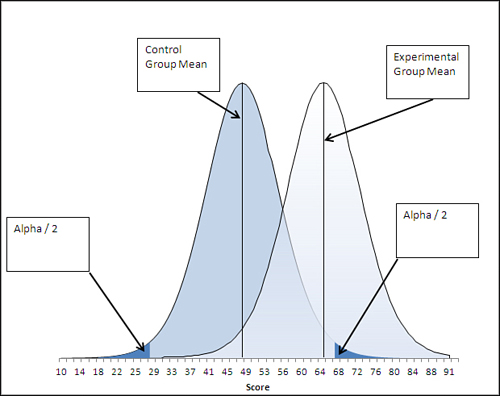
You put all 5% of the alpha into the left tail of the distribution that represents the null hypothesis, as shown in Figure 8.7, and doing so results in a critical value of 46. A sample mean above 46 means that you continue to regard the null hypothesis as tenable (while recognizing that you might be missing a genuine difference). A sample mean below 46 means that you reject the null hypothesis (while recognizing that you might be doing so erroneously).

But what if you get a sample mean of 64? That’s as far above the null hypothesis mean of 55 as the critical value of 46 is below it. Given your null hypothesis that the Gulf mean and the population mean are both 55, isn’t it as unlikely that you’d get a sample mean of 64 as that you’d get one of 46?

Yes, it is, but that’s irrelevant. When you adopted your alternative hypothesis, you made it a directional one. Your alternative stated that the mean age of Gulf turtles is less than, not equal to, and not more than, the mean age of the rest of the world’s population of turtles. And you adopted a 0.05 alpha level.

Now you obtain a sample mean of 64. If you therefore reject your null hypothesis, you are changing your alpha level after the fact. You are changing it from 0.05 to 0.10, because you are putting half your alpha into the left tail of the distribution that represents the null hypothesis, and half into the right tail. Because 5% of the distribution is in the left tail, 5% must also be in the right tail, and your total alpha is not 0.05 but 0.10.

Okay, then why not change things so that the left tail contains 2.5% of the area under the curve and the right tail does too? Then you’re back to a total alpha level of 5%.

But then you’ve changed the critical value. You’ve moved it farther away from the mean, so that it cuts off not 5% of the area under the curve, but 2.5%. And the same comment applies to the right tail. The critical values are now not 46 and 64, but 44 and 66, and you can’t reject the null hypothesis whether you get a sample mean of 45 or 65.

You can see the kind of logical and mathematical difficulties you can get into if you don’t follow the rules. Decide whether you want to make a directional or nondirectional hypothesis. Decide on an alpha level. Make those decisions before you start seeing results, and stick with them. You’ll sleep better. And you won’t leave yourself open to a charge that you stacked the deck.

Using Hypotheses to Guide Excel’s t-Distribution Functions

This section shows you how to choose an Excel function to best fit your null and alternative hypotheses. The previous chapter’s example entailed a single group t-test, which compared a sample mean to a hypothetical value. This section discusses a slightly more complicated example, which involves not one but two groups.

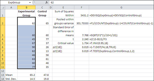
Figure 9.1 shows scores on a paper-and-pencil driving test, in cells B2:C11. Participants, who were all ticketed for minor traffic infractions, were selected randomly and randomly assigned to either an experimental group that attended a class on traffic laws or a control group that did nothing special.

Figure 9.1. Note from the Name box that the range B2:B11 has been named ExpGroup.

Making a Directional Hypothesis

Suppose first that the researcher believes that the class could have increased the test scores but could not have decreased them. The researcher makes the directional hypothesis that the experimental group will have a larger mean than the control group. The null hypothesis is that there is no difference between the groups as assessed by the test.

The researcher also decides to adopt a 0.05 alpha rate for the experiment. It costs $100 per student to deliver the training, but the normal procedures such as flagging a driver’s license cost only $5 per participant. Therefore, the researcher wants to hold the probability of deciding the program has an effect, when it really doesn’t, to one chance in 20, which is equivalent to an alpha rate of 0.05.

After the class was finished, both groups took a multiple choice test, with the results shown in Figure 9.1.

This researcher believes in running a t-test by taking the long way around, and there’s a lot to be said for that. By taking things one step at a time, it’s possible to look at the results of each step and see if anything looks irrational. In turn, if there’s a problem, it’s easier to diagnose, find, and fix if you’re doing the analysis step by step.

Here’s an overview of what the researcher does at this point. Remember that the alpha level has already been chosen, the directionality of the hypothesis has been set (the experimental group is expected to do better, not just differently, on the test than the control group), and the data has been collected and entered as in Figure 9.1. These are the remaining steps:

1. For convenience, give names to the ranges of scores in B2:B11 and C12:C11 in Figure 9.1.
2. Recalling from Chapter 3, “Variability: How Values Disperse,” that the variance is the average squared deviation from the mean, calculate and total up the squared deviations from each group’s mean.
3. Get the pooled variance from the squared deviations calculated in step 2.
4. Calculate the standard error of the mean differences from the pooled variance.
5. Calculate the t-statistic using the observed mean difference and the result of step 4.
6. Use T.INV() to obtain the critical t-statistic.
7. Compare the t-statistic to the critical t-statistic. If the computed t-statistic is smaller than the critical t-statistic for an alpha of 0.05, regard the null hypothesis as tenable. Otherwise, reject the null hypothesis.

The next few sections explore each of these seven steps in more detail.

Step 1: Name the Score Ranges

To make it easier to refer to the data ranges, begin by naming them. There are various ways to name a range, and some ways offer different options than others. The simplest method is the one used here. Select the range B2:B11, click in the Name box (at the left end of the Formula Bar), and type the name ExpGroup. Press Enter. Select C2:C11, click in the Name box, and type the name ControlGroup. Press Enter.

Step 2: Calculate the Total of the Squared Deviations

You are after what’s called a pooled variance in order to carry out the t-test. You have two groups, the experimental and the control, and each has a different mean. According to the null hypothesis, both groups can be thought of as coming from the same population, and differences in the group means and the group standard deviations are due to nothing more than sampling error.

However, much of the sampling error that exists can be mitigated to some degree by pooling the variability in each group. That process begins by calculating the sum of the squared deviations of the experimental group scores around their mean, and the sum of the squared deviations of the control group scores around their mean.

Excel provides a worksheet function to do this: DEVSQ(). The formula

=DEVSQ(B2:B11)

calculates the mean of the values in B2:B11, subtracts each of the ten values from their mean, squares the results, and totals them. If you don’t trust me, and if you don’t trust DEVSQ(), you could instead use this array formula (don’t forget to enter it with Ctrl+Shift+Enter):

=SUM((B2:B11-AVERAGE(B2:B11))∧2)

Using the names already assigned to the score ranges, the formula

=DEVSQ(ExpGroup)+DEVSQ(ControlGroup)

returns the total of the squared deviations from the experimental group’s mean, plus the total of the squared deviations from the control group’s mean.

The result of this step appears in cell F1 of Figure 9.1. The formula itself, entered as text, is shown in cell G1.

Step 3: Calculate the Pooled Variance

Again, the variance can be thought of as the average of the squared deviations from the mean. We can calculate a pooled variance using the total squared deviations with this formula:

=F1/(COUNT(ExpGroup)−1+COUNT(ControlGroup)−1)

That formula uses the sum of the squared deviations, in cell F1, as its numerator. The formula divides that sum by the number of scores in the Experimental group, plus the number of scores in the Control group, less one for each group.

That’s why I just said that the variance “can be thought of” as the average squared deviation. It can be helpful conceptually to think of it in that way. But using Excel’s COUNT() function, you divide by the group size minus 1, instead of by the actual count, so the computed variance is not quite equal to the conceptual variance. The difference becomes smaller and smaller as the group size increases, of course.

If you think back to Chapter 3, which discussed the reason to divide by the degrees of freedom instead of by the actual count, you’ll recall that the formula loses one degree of freedom because calculating the mean (and sticking to that mean as the deviations are calculated) exerts a constraint on the values. In this case, we’re dealing with two groups, hence two means, and we lose two (not just one) degrees of freedom in the denominator of the variance.

Step 4: Getting the Standard Error of the Difference in Means

Let’s recall Chapter 3 once again: The standard error of the mean is a special kind of standard deviation. It is the standard deviation that you would calculate if you took samples from a population, calculated the mean of each sample, and then calculated the standard deviation of those means. Although that’s the definition, you can estimate the standard error of the mean from just one sample: It is the standard deviation of your single sample divided by the square root of its sample size. Similarly, you can estimate the variance error of the mean by dividing the variance of your sample by the sample size.

The standard error of the mean is the proper divisor to use when you have only one mean to test against a known or hypothesized value, such as the example in Chapter 8 where the mean of a sample was tested against a known population parameter.

In the present case, though, you have two groups, not just one, and the proper divisor is not the standard error of the mean, but the standard error of the difference between two means. That is the value that the first steps in this process have been working toward. As a result of step 3, you have the pooled within-groups variance.

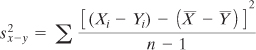
To convert the pooled variance to the variance error, you must divide the pooled within-groups variance by the sample sizes of both groups. Because, as you’ll see, the groups may consist of different numbers of subjects, the more general formula is as follows, where N as usual indicates the sample size:

(The formula, of course, simplifies if both groups have the same number of subjects. And as you’ll also see, an equal number of subjects also makes the interpretation of the statistical test more straightforward.)

That prior equation returns the variance error of the difference between two means. To get the standard error of the difference, as shown in cell F3 of Figure 9.1, simply take its square root:

Step 5: Calculate the t-Statistic

This step takes less time than any other, assuming that you’ve done the proper groundwork. Just subtract one group mean from the other and divide the result by the standard error of the mean difference. You’ll find the formula and the result for this example, 2.24, in cell F4 of Figure 9.1.

It’s an easy step to take but it’s one that masks some minor complexity, and that can be a little confusing at first. Except in the very unlikely event that both groups have the same mean value, the t-statistic will be positive or negative depending on whether you subtract the larger mean from the smaller or vice versa.

It can happen that you’ll get a large, negative t-statistic when your hypotheses led you to expect either a positive one or no reliable difference. For example, you might test an auto tire that you expect to raise mileage, and you phrase your alternative hypothesis accordingly. But when the results come in and you subtract the control group mean mpg from the experimental group mean mpg, you wind up with a negative number, hence a negative t-statistic. It gets worse if the t-statistic is something like −5.1: a value that is highly improbable if the null hypothesis is true.

That kind of result is more likely due to confused logic or incorrect math than it is to an inherently improbable research outcome. So, if it occurs, the first thing you should do is verify that you phrased your hypotheses to conform to your understanding of the treatment effect. Then you should check your math—including the way that you presented the data to Excel’s functions and tools. If you’ve handled those matters correctly, all you can do is swallow your surprise, continue to entertain the null hypothesis, and plan your next experiment using the knowledge you’ve gained in the present one.

Be careful about this sort of thing if and when you use the Data Analysis t-test tools. They subtract whatever values you designate as Variable 2 from the values you designate as Variable 1. It doesn’t matter to that tool whether your alternative hypothesis is that Variable 2’s mean will be larger, or Variable 1’s. Variable 2 is always subtracted from Variable 1. It’s helpful to be aware of this when you apply the Variable 1 and Variable 2 designations.

Step 6: Determine the Critical Value Using T.INV()

You need to know the critical value of t: the value that you’ll compare to the t-statistic you calculated in step 5. To get that value, you need to know the degrees of freedom and the alpha level you have adopted.

The degrees of freedom is easy. It’s the denominator of the standard error of the mean difference: that is, it’s the total sample size of both groups, minus 2. This example has ten observations in each group, so the degrees of freedom is 10 + 10 − 2, or 18.

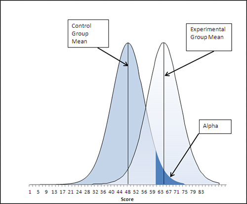
You have already specified an alpha of 0.05 and a directional alternative hypothesis that states the experimental group will have a higher mean than the control group. The situation appears graphically in Figure 9.2.

Figure 9.2. This directional hypothesis places all of alpha in the right tail of the left distribution.

To find the value that divides the alpha area from the rest of the left distribution, enter this formula:

=T.INV(0.95,18)

That formula returns 1.73, the critical value for this situation, the smallest value that your calculated t-statistic can be if you are to reject the null hypothesis at your chosen level of alpha.

Notice that your alpha is .05 but the formula uses .95 as the first argument to the T.INV() function. The T.INV() function (as well as the TINV() compatibility function) returns the t value for which the percent under the curve lies to the left. In this case, 95% of the area of the t-distribution with 18 degrees of freedom lies to the left of the t value 1.73. Therefore, 5% of the area under the curve lies to the right of 1.73, and that 5% is your alpha rate.

To convert the t value to the scale of measurement used on the chart’s horizontal axis, just multiply the t value by the standard error of the mean differences and add the control group mean. Those values are shown in Figure 9.1, in cells F3 (standard error) and C13 (control mean). The result is a value of 61, in this example’s original scale of measurement.

Suppose that your treatment was not intended to improve drivers’ scores on a test on traffic laws but their golf scores. Your null hypothesis, as before, would probably be that the post-treatment mean scores are the same, if the treatment were administered to the full population. But your alternative hypothesis might well be that the treatment group’s mean score is lower than that of the control group. With the same alpha rate as before, 0.05, the change in the direction of your alternative hypothesis is shown in Figure 9.3.

Figure 9.3. The experimental group’s mean still exceeds the critical value.

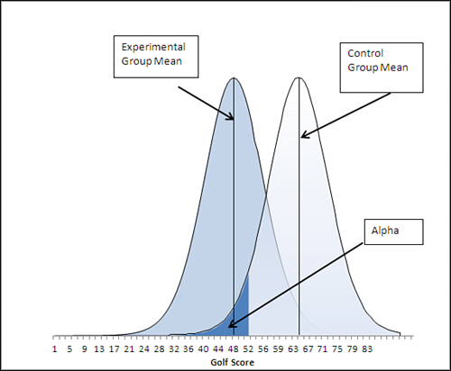
Now, the critical value of t that divides the alpha area from the rest of the area under the control group’s distribution of sample means has 5% of the area to its left, not 95% as in the prior example. You can find out what the t value is by using this formula:

=T.INV(.05,18)

The alpha rate is the same in both examples, and both examples use a directional hypothesis. The degrees of freedom is the same in both cases. The sole difference is the direction of the alternative hypothesis—in Figure 9.3 you expect the experimental group’s mean to be lower, not higher, than that of the control group.

One way to deal with this situation is as shown in Figure 9.3. The area that represents alpha is placed in the left tail of the control group’s distribution, bordered by the critical value that separates the 5% alpha area from the remaining 95% of the area under the curve. When you want 5% of the area to appear to the left of the critical value, you would use 0.05 as the first argument to T.INV(). When you want 95% of the area to appear to the left of the critical value, use 95% as the first argument. T.INV() responds with the critical value that you specify with the probability you’re interested in, along with the degrees of freedom that defines the shape of the curve.

The t-distribution has a mean of zero and it is symmetric (although, as Chapter 8 discussed, it is not the same as the normal distribution). Earlier in this section you saw that the formula

=T.INV(0.95,18)

returns 1.73. Because the t-distribution has a zero mean and is symmetric, the formula

=T.INV(0.05,18)

returns −1.73. Either 1.73 or −1.73 is a critical value for a t-test with an alpha of 5% and 18 degrees of freedom.

I included Figure 9.3 and the related discussion of the placement of the area that represents alpha primarily to provide a better picture of where and how your hypotheses affect the placement of alpha. This chapter gets more deeply into that matter when it takes up nondirectional hypotheses.

But suppose you’re in a situation such as the one shown in Figure 9.3. As it’s set up, you might subtract the (larger) control group mean from the (smaller) experimental group mean and compare the result to the critical value of −1.73. If you got a calculated t-statistic that is farther from 0 than −1.73, you would reject the null hypothesis.

But you could also adopt the viewpoint that things are as shown in Figure 9.2, except that the labels for the experimental and control group are swapped. Your alternative hypothesis could just as well state that the control group mean is greater than the experimental group. If you do that, alpha is located where it is in Figure 9.2 and you need not deal with negative critical values for t.

Step 7: Compare the t-Statistic to the Critical t-Statistic

You calculated the observed t-statistic as 2.24 in step 5. You obtained the critical value of 1.73 in step 6. Your observed t-statistic is larger than the critical value and so you reject the null hypothesis with 95% confidence (that 95% is, of course, 1 − alpha).

Completing the Picture with T.DIST()

So far this section has discussed the use of the T.INV() function to get a critical value, given an alpha and degrees of freedom. The other side of that coin is represented by the T.DIST(), the T.DIST.RT(), and the T.DIST.2T() functions.

When you use one of those three T.DIST functions, you specify a critical value rather than an alpha value. You still must supply the degrees of freedom. Here’s the syntax for T.DIST():

=T.DIST(x, df, cumulative)

where x is a t value, df is the degrees of freedom, and cumulative specifies whether you want all the area under the curve to the left of the t-statistic or the probability associated with that t-statistic itself (that’s the relative height of the curve at the point defined by the t statistic). So, using the figures from the prior section, the formula

=T.DIST(1.73,18,TRUE)

returns 0.95. Ninety-five percent of the area under a t-distribution with 18 degrees of freedom lies to the left of a t value of 1.73.

Because the t-distribution is symmetric, both the formulas

=1 - T.DIST(1.73,18,TRUE)

and

=T.DIST(-1.73,18,TRUE)

return 0.05, and you might want to use them if your hypotheses were as suggested in Figure 9.3—that is, alpha is in the left tail of the control group’s distribution. If your situation were similar to that shown in Figure 9.2, with alpha in the right tail of the control group distribution, you might find it more convenient to use this form of T.DIST():

=T.DIST.RT(1.73,18)

It also returns 0.05. Using the .RT as part of the function’s name indicates to Excel that you’re interested in the area in the right tail of the t-distribution. Notice that there is no cumulative argument as there is in T.DIST(). The function assumes that you want to obtain the cumulative area to the right of the critical value. Again, because of the symmetry of the t-distribution, you can get the curve’s height at 1.73 by using this (which you would also use for its height at −1.73):

=T.DIST(1.73,18,FALSE)

The final form of the T.DIST() function is T.DIST.2T(), which returns the combined areas in the left and right tails of the t distribution. It’s useful when you are making a nondirectional hypothesis (see Figure 9.5 in the next section). The syntax is

=T.DIST.2T(x, df)

where, again, x refers to the t value and df to the degrees of freedom, and there is no cumulative argument. This usage of the function

=T.DIST.2T(1.73,18)

returns 0.10. That’s because 5% of the area under the t-distribution with 18 degrees of freedom lies to the right of 1.73, and 5% lies to the left of −1.73. I do not believe you will find that you have much use for T.DIST.2T, in large measure because with nondirectional hypotheses you are as interested in a negative t value as a positive one, and T.DIST.2T, like the pre-2010 function TDIST(), cannot cope with a negative value as its first argument. It is more straightforward to use T.DIST() and T.DIST.RT().

Using the T.TEST() Function

The T.TEST() function is a quick way to arrive at the probability of a t-statistic that it calculates for you. In that sense, it differs from T.DIST(), which requires you to supply your own t-statistic and degrees of freedom; then, T.DIST() returns the associated probability. And T.INV() returns the t-value that’s associated with a given probability and degrees of freedom.

Regardless of the function you want to use, you must always supply the degrees of freedom, either directly in T.DIST() and T.INV() or indirectly, as you’ll see, in T.TEST(). The next section discusses how degrees of freedom in two-group tests differs from degrees of freedom in Chapter 8’s one-group tests.

Degrees of Freedom in Excel Functions

Regardless of the Excel function you use to get information about a t-distribution, you must always specify the number of degrees of freedom. As discussed in Chapter 8, this is because t-distributions with different degrees of freedom have different shapes. And when two distributions have different shapes, the areas that account for, say, 5% of the area under the curve have different boundaries, also termed critical values.

For example, in a t-distribution with 5 degrees of freedom, 5% of its area lies to the right of a t-statistic of 2.01. In a t-distribution with six degrees of freedom, 5% of its area lies to the right of a t-statistic of 1.94. (As the number of degrees of freedom increases, the t-distribution becomes more and more similar to the normal distribution.)

So you must tell Excel how many degrees of freedom are involved in your particular t-test. When you estimate a population standard deviation from a sample, the sample size is N and the number of degrees of freedom is N − 1. The degrees of freedom in a t-test is calculated similarly.

In the case of a t-test, N means the number of cases in a group. So if you are testing the mean of one sample against a hypothesized value (as was done in Chapter 8), the degrees of freedom to use in the t-test is the number of records in the sample, minus one. If you are testing the mean of one sample against the mean of another sample (as was done in the prior section), the degrees of freedom for the test is N₁ + N₂ − 2: You lose one degree of freedom for each group’s mean.

Equal and Unequal Group Sizes

There is no reason you cannot run a t-test on groups that contain different numbers of observations. That statement applies no matter whether you use T.DIST() and T.INV() or T.TEST(). If you work your way once again through the examples provided in this chapter’s first section, you’ll see that there is no calculation that requires both groups to have the same number of cases.

However, there are two issues that pertain to the use of equal group sizes in t-tests. These are discussed in detail later in this chapter, but here’s a brief overview.

Dependent Groups t-Tests

Sometimes you want to use a t-test on two groups whose members can be paired in some way. For example, you might want to compare the mean score of one group of people before and after a treatment. In that case, you can pair Joe’s pretest score with his posttest score, Mary’s pretest score with her posttest score, and so on.

If you take to heart the discussion of experimental design in Chapter 6, “Telling the Truth with Statistics,” you won’t regard a simple pretest-posttest comparison as necessarily a valid experiment. But if you have arranged for a proper comparison group, you can run a t-test on the pretest scores versus the posttest scores. The t-test takes the pairing of observations into account. And because each pretest score can be paired with a posttest score, your two groups by definition have the same number of observations—you’ll see next why that’s important.

Other ways that you might want to pair the observations in two groups include family relationships such as father-son and brother-sister, and members of pairs matched on some other variable who are then randomly assigned to one of the two groups in the t-test.

The Data Analysis add-in has a tool that performs a dependent groups t-test. The add-in refers to it as T-Test: Paired Two Sample for Means.

Unequal Group Variances

One of the assumptions of the t-test is that the populations from which the two groups are drawn have the same variance. Although that assumption is made, both empirical research and theoretical work have shown that violating the assumption makes little or no difference when the two groups are the same size.

However, suppose that the two populations have different variances—say, 30 and 10. If the two groups have different sample sizes and the larger group is sampled from the population with the larger variance, then the probability of mistakenly rejecting a true null hypothesis is smaller than T.DIST() would lead you to expect. If the larger group is sampled from the population with the smaller variance, the probability of mistakenly rejecting a true null hypothesis is larger than you would otherwise expect.

Figure 9.4 shows what can happen.

Figure 9.4. Different group sizes and different variances combine to increase or decrease the standard error of mean differences.

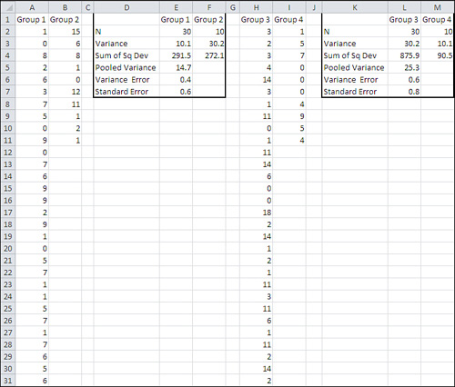
Individual scores in columns A and B are summarized in columns D through F. Group 1 has 30 observations and a variance of 10.0; Group 2 has 10 observations and a variance of 30.1. The larger group has the smaller variance.

Individual scores in columns H and I are summarized in columns L and M. Groups 3 and 4 have the same numbers of observations as 1 and 2, but their variability has been reversed: the larger group now has the larger variance.

Even though the group sizes are the same in both instances, and the variances are the same size, the standard error of the difference in means is noticeably smaller in cell E7 than it is in cell L7. That results in an underestimate of the standard error in the population. Group 1 has three times the observations as Group 2, and therefore its lower variability has a greater effect on the standard error in row 7 than does Group 2’s larger variability. The net effect is, in the long run, an underestimate of the standard error in the population.

When the standard error is smaller, you do not need as large a difference between means to conclude that the observed difference is reliable, and that you are in the region of the curve where you will reject the null hypothesis. (See Figure 9.12 for a demonstration of that effect.) Because you tend to be working with an underestimate of the population variability in this situation—larger group, smaller variance—you will conclude that the difference is reliable more often than you think you will when the null hypothesis is false.

Now consider the situation shown in columns H through M in Figure 9.4. The larger group now has the larger variance. Because it has more observations, it once again contributes more of its variability to the eventual standard error calculation in cell L7. The effect is to make the standard error larger than otherwise; in fact, it is 25% larger than in cell E7.

Now the standard error will be larger than in the population in the long run. You will reject the null hypothesis less frequently than you think you will when it is false.

I have made the differences in group sizes and variances fairly dramatic in this example. One group is three times as large as the other, and one variance is three times as large as the other. These are differences that you’re unlikely to encounter in actual empirical research. Even if you do, the effect is not a large one. However, it could make a difference, and Excel’s T.TEST() function has an accepted method of handling the situation. See the subsequent section, “Using the Type Argument” for more information.

The Data Analysis add-in has a tool that incorporates the latter method. It is named T-Test: Two-Sample Assuming Unequal Variances.

Notice that because a dependent groups t-test by definition uses two groups that have equal sample sizes, the issue of unequal variances and error rate doesn’t arise. Having equal group sizes means that you don’t need to worry about the equal variance assumption.

The T.TEST() Syntax

The syntax for the T.TEST() function is

=T.TEST(Array1, Array2, Tails, Type)

This syntax is quite different from that for T.DIST() and T.INV(). There is no x argument, which is the t value that you supply to T.DIST(), and there is no probability argument, which is the area that you supply to T.INV(). Nor is there a degrees of freedom argument, as there is for both T.DIST() and T.INV().

The reason that those arguments are missing in T.TEST() is that you tell Excel where to find the raw data. If you were using T.TEST() with the problem shown in Figure 9.1, for example, you might supply B2:B11 as the Array1 argument, and C2:C11 as the Array2 argument. The fact that you are supplying the raw data to the T.TEST() function has these results:

• The T.TEST() function is capable of doing the basic calculations itself. It can count the degrees of freedom because it knows how many values there are in Array1 and Array 2.

• It can calculate the pooled within-groups variance and the standard error of the mean differences. It can calculate the mean of each array. Therefore, it can calculate a t-statistic.

• Because it can calculate the t-statistic and degrees of freedom itself by looking at the two arrays, T.TEST() can and does return the probability of observing that calculated t-statistic in a t-distribution with that many degrees of freedom.

Identifying T.TEST() Arrays

The T.TEST() function returns only a probability level: the probability that you would observe a difference in the means of two groups as large as you have observed, assuming that there is no difference between the groups in the populations from which the samples came (in the example shown in Figure 9.1, between people who get the training and people who don’t).

With the data as shown in Figure 9.1, you could enter this formula in some blank cell (in that figure it’s in cell F6):

=T.TEST(ExpGroup,ControlGroup,1,2)

Array1 and Array2 are two arrays of values whose means are being compared. In the example, Array1 is a range of cells that has been given the name ExpGroup; that range is B2:B11. Array2 is a range of cells that has been given the name ControlGroup, and it’s C2:C11. The means and standard deviations of the two groups, calculated separately using the AVERAGE() and STDEV.S() functions, are in the range B13:C14. They are there strictly for your information; they have nothing to do with the T.TEST() function or its use.

Using the Tails Argument

The Tails argument concerns the directionality of your hypotheses. The present example assumes that the treatment will not decrease the score on a traffic test, compared to a control group. Therefore, the researcher expects that the experimental group will score well enough on the test that the only concern is whether the experimental mean is high enough that chance can be ruled out as an explanation for the outcome. The hypothesis is directional.

This situation is similar to the hypotheses that were used in the prior section, in which the experimenter believed that the treatment would leave the experimental group higher (or lower) on the outcome measure than the control group. The hypotheses were directional.

If the experimenter’s alternative hypothesis were that the experimental group’s mean would be different from that of the control group (not higher than or lower than, just different), then the alternative hypothesis is nondirectional.

Setting the Tails Argument to 1

In Figure 9.2, the experimenter has adopted .05 as alpha. The right tail of the left curve contains all of alpha, which is .05 or 5% of the area under the left curve. Figure 9.2 is a visual representation of the experimenter’s decision rule, which in words is this:

Given the data shown in Figure 9.1, the experimenter rejects the null hypothesis that the two means are the same. The alternative hypothesis is therefore tenable: that the experimental mean in the full population is greater than the control mean in the full population.

Notice the value 0.019 in cell F7 of Figure 9.1. It shows the result of the T.TEST() function. Cell G7 shows that the function’s third argument, Tails, is equal to 1. That tells Excel to report the error probability in one tail only. So when Excel reports the result of T.TEST() at 0.019, it is saying that, in this example, 1.9% of the area is found above, and only above, the experimental group mean.

Interpreting the T.TEST() Result

It’s important to recognize that the value returned by T.TEST() is not the same as alpha, although the two quantities are conceptually related. As the experimenter, you set alpha to a value such as .01, .025, .05, and so on.

In contrast, the T.TEST() function returns the percentage of the left curve that falls to the right of the right curve’s mean. That percentage might be less than or equal to alpha, in which case you reject the null hypothesis; or it might be greater than alpha, in which case you continue to regard the null hypothesis as tenable.

In Figure 9.2, the value 0.019 is represented as the area under the left, control group curve that exceeds the experimental group mean. Only 1.9% of the time would you get an experimental group mean as large as this one when the experimental and control population means were really the same.

The experimenter set alpha at .05. The experimental group’s mean was even farther from the control group’s mean than is implied by an alpha of .05 (the critical value that divides the charted alpha region from the rest of the control group’s distribution). So the experimenter can reject the null hypothesis at the .05 level of confidence—not at the .019 level of confidence. Once you have specified an alpha and an alternative hypothesis, you stick with it.

For example, suppose that the experimental group’s mean score had been not 65.2 but 30.4. That’s as far below the control group mean as the actual result is above the control group mean. Is that a “statistically significant” finding? In a sense, yes it is. It would occur at about the same 1.9% of the time that the actual finding did, given that the means are equal in the populations.

But the experimenter adopted the alternative hypothesis that the experimental group’s mean would be higher than the treatment group’s mean. That alternative implied that the error rate, the entire .05 or 5%, should be put in the right tail of the control group’s curve. An experimental group mean of 30.4 does not exceed the minimum value for that alpha region, and so the alternative hypothesis must be rejected. The null hypothesis, that the group means are equal, must be retained even though a startlingly low experimental group mean came about.

Setting the Tails Argument to 2

Now suppose that the experimenter had a somewhat more modest view of the treatment effect, and admitted it’s possible that instead of raising the experimental group’s scores, the treatment might lower them. In that case, the null hypothesis would remain the same—that the population means are the same—but the alternative hypothesis would be different. Instead of stating that the experimental group mean is higher than the control group mean, the alternative hypothesis would state that it is different from the control group mean: that is, either higher or lower than the control group mean, and the experimenter won’t predict which.

Figure 9.5 illustrates this concept.

Figure 9.5. The area that represents alpha is divided between the two tails of the distribution that represents the control group sample mean.

Figure 9.5 represents a nondirectional decision rule. Here it is in words:

This is called a nondirectional test because the experimenter is not setting an alternative hypothesis that states that the experimental mean will be higher than the mean of the control group; nor does the alternative state that the experimental mean will be lower. All the alternative hypothesis states is that the two means will be different beyond an amount that can be reasonably attributed to chance. The test is also sometimes termed a two-tailed test because the error rate, alpha, is split between the two tails of the curve that represents the possible control group sample means. In this example, alpha is still .05, but .025 is in the left tail and .025 is in the right tail.

In this situation, the experimenter can reject the null hypothesis if the experimental group’s mean falls below the lower critical value or above the upper critical value. This differs from the decision rule used with directional hypotheses, which can force the experimenter to regard the null hypothesis as tenable even though the experimental mean might fall improbably far from the control group mean, in an unexpected direction.

There’s a cost to nondirectional tests, though. Nondirectional tests allow for more possibilities than directional tests, but their statistical power is lower. Compare the upper critical value in Figure 9.2 with that in Figure 9.5. In Figure 9.2, the directional test puts all of alpha into the right tail, and so doing places the critical value at about 61. In Figure 9.5, the nondirectional test puts only half of alpha, .025, into the right tail, and so doing raises the critical value from about 61 to a little over 67.

When a critical value moves away from the mean of the sampling distribution that represents the comparison group, the power of the statistical test is reduced. Compare Figures 9.6 and 9.7.

Figure 9.6. The experimental group mean exceeds the critical value because the entire alpha is allocated to the right tail of the left curve.

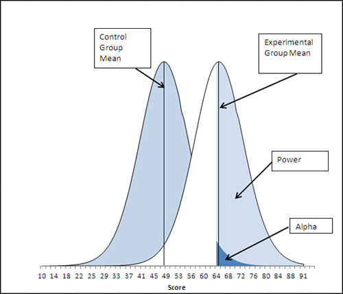
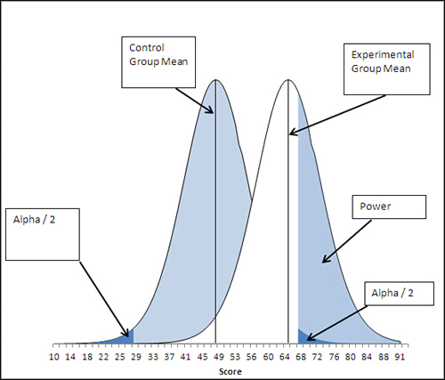
Figure 9.7. The upper critical value has moved right, reducing power, because alpha has been divided between two tails of the left curve.

In Figure 9.6, notice that the experimental group mean is just barely above the critical value of 64: It’s within the region defined by the statistical power of this t-test, so the test has enough sensitivity to reject the null hypothesis.

In Figure 9.7, the experimenter has made a nondirectional hypothesis. If alpha remains at .05, this means that .025 instead of .05 of the area under the left curve defines the upper critical value. That moves the critical value to the right, as compared to the situation depicted in Figure 9.6, and in turn that reduces the test’s statistical power.

In general, making a directional hypothesis increases a test’s statistical power when the experimenter has good reason to expect that the outcome will favor one group or the other. The tradeoff is that a directional hypothesis won’t support a decision to reject the null when the experimental group’s mean differs from the control group’s mean, but in an unexpected direction.

Again, the syntax of the T.TEST() function is as follows:

=T.TEST(Array1, Array2, Tails, Type)

In the T.TEST() function, you state whether you want Excel to examine one tail only or both tails. If you set Tails to 1, Excel returns the area of the curve beyond the calculated t statistic in one tail. If you set Tails to 2, Excel returns the total of the areas to the right of the t statistic and to the left of the negative of the t-statistic. So if the calculated t is 3.7, T.TEST() with two tails returns the area under the curve to the left of -3.7 plus the area to the right of +3.7.

Using the Type Argument

The fourth Type argument to the T.TEST() function tells Excel what kind of t-test to run, and your choice involves some assumptions that this chapter has as yet just touched on.

Most tests that support statistical inference make assumptions about the nature of the data you supply. These assumptions are usually due to the mathematics that underlies the test. In practice:

• You can safely ignore some assumptions.

• Some assumptions get violated, but there are procedures for dealing with the violation.

• Some assumptions must be met or the test will not work as intended.

The Type argument in the T.TEST() function pertains to the second sort of assumption: When you specify a Type, you tell Excel which assumption you’re worried about and thus which procedure it should use to deal with the violation.

The theory of t-tests makes three distinct assumptions about the data you have gathered.

Normal Distributions

The t-test assumes that both samples are taken from populations that are distributed normally on the measure you are using. If your outcome measure were a nominal variable such as Ill versus Healthy, you would be violating the assumption of normality because there are only two possible values and the measure cannot be distributed normally.

This assumption belongs to the set that you can safely ignore in practice. Considerable research has investigated the effect of violating the normality assumption and it shows that the presence of underlying, non-normal distributions has only a trivial effect on the results of the t-test. (Statisticians sometimes say that the t-test is robust with respect to the violation of the assumption of normality, and the studies just mentioned are referred to as the robustness studies.)

Independent Observations

The t-test assumes that the individual records are independent of one another. That is, the assumption is that the fact that you have observed a value in one group has no effect on the likelihood of observing another value in either group.

Suppose you were testing the status of a gene. If Fred and Judy are brother and sister, the status of Fred’s gene might well mirror the status of Judy’s gene (and vice versa). The observations would not be independent of one another, whether they were in the same group or in two different groups.

This is an important assumption both in theory and in practice: The t-test is not robust with respect to the violation of the assumption of independence of observations. However, you often find that quantifiable relationships exist between the two groups.

For example, you might want to test the effect of a new type of car tire on gas mileage. Suppose first that you acquire, say, 20 new cars of random makes and models and assign them, also at random, to use either an existing tire or the new type. But with that small a sample, random assignment is not necessarily an effective way to equate the two groups of cars.

Now suppose that you acquire two cars from each of ten different model lines. Then you randomly assign one car from each model-pair to get four tires of an existing type, and the other car in the pair to get four tires of your new type. The layout of this experiment is shown in Figure 9.8.

Figure 9.8. As you saw in Chapter 4, “How Variables Move Jointly: Correlation,” you can pair up observations in a list by putting them in the same row.

In this design, the observations clearly violate the assumption of independence. The fact that one car from each model has been placed in one group means that the probability is 100% that another car, identical but for the tires, is placed in the other group. Because the only difference between the members of a matched pair is the tires, the two groups have been equated on other variables, such as weight and number of cylinders.

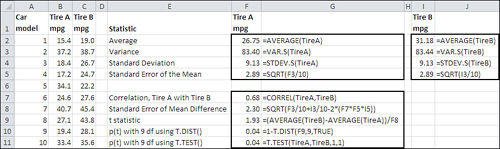
And because the experimenter can pair up the observations, the amount of dependence between the two groups can be calculated and used to adjust the t-test. As is shown in Figure 9.8, the correlation in gas mileage between the two groups is a fairly high 0.68; therefore, the R-squared, the amount of shared variance in gas mileage, is almost 47%.

Because of the pairing of observations in different groups, the dependent groups t-test has one degree of freedom for each pair, minus 1. So in the example shown in Figure 9.8, the dependent groups t-test has 10 pairs minus 1, or 9 degrees of freedom.

Figure 9.8 also shows the result of the T.TEST() function on the two arrays in columns B and C. With nine degrees of freedom, taking into account the correlation between the two groups, the likelihood of getting a sample mean difference of 4.43 miles per gallon is only .04, if there is no difference in the underlying populations. If you had started out by setting your alpha rate to .05, you could reject the null hypothesis of no difference.

Calculating the Standard Error for Dependent Groups

One of the reasons to use a dependent groups t-test when you can do so is that the test becomes more powerful, just as using a larger value of alpha or making a directional hypothesis makes the t-test more powerful. To see how this comes about, consider the way that the standard error of the difference between two means is calculated.

Here is the formula for the variance of a variable named A:

Then, if A is actually equal to X − Y, we have the following:

Rearranging the elements in that expression results in this:

Expanding that expression by carrying out the squaring operation, we get this:

The first term here is the variance of X. The third term is the variance of Y. The second term includes the covariance of X and Y (see Chapter 4 for information on the covariance and its relationship to the correlation coefficient.) So the equation can be rewritten as

or

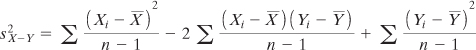
Therefore, the variance of the difference between two variables can be expressed as the variance of the first variable plus the variance of the second variable, less twice the covariance. Chapter 4 also discusses the covariance as the correlation between the two variables times their standard deviations.

The only part of that you should bother to remember is that you subtract a quantity that depends on the strength of the correlation between the two variables. In the context of the dependent groups t-test, those variables might be the scores of the subjects in Group 1 and the scores of their siblings in Group 2—or the mpg attained by the car models in Group 1 and the mpg for the identical models in Group 2, and so on.

It’s worth noting that when you are running an independent groups t-test, as was done in the first part of this chapter, there is no correlation between the scores on the two groups. Then the standard error of the mean differences is just the sum of the groups’ variances. With equal sample sizes, the sum of the groups’ variances is the same as the pooled variance discussed earlier in the chapter.

But when members of the two groups can be paired up, you can calculate a correlation and reduce the size of the standard error accordingly (refer to the final equation). In turn, this gives your test greater power. To review, here’s the basic equation for the t-statistic:

Clearly, when the denominator is smaller, the ratio is larger. A larger t-statistic is more likely to exceed the critical value. Therefore, when you can pair up members of two groups, you can calculate the correlation on the outcome variable between the two groups. That results in a smaller denominator, because you subtract it (multiplied by 2 and by the product of the standard deviations) from the sum of the variances.

In a case such as the car tire example, you expect that the observations are not independent, but because you can pair up the dependent records (each model of car is represented once in each group), you can quantify the degree of dependency—that is, you can calculate the correlation between the two sets of scores because you know which score in one group goes with which score in the other group. Once you have quantified the dependency, you can use it to make the statistical test more sensitive.

That is the purpose of one of the values you can select for the T.TEST() function’s Type argument. If you supply the value 1 as its Type argument, you inform Excel that the records in the two arrays are related in some way and that the correlation should factor into the function’s result. So if each array contains one of two twins, then Record 1 in one array should be related to Record 1 in the second array; Record 2 in one array should be related to Record 2 in the other array, and so on.

Running the Car Example Two Ways

Figure 9.8 shows how you can run a dependent groups t-test two different ways. One way grinds the analysis out formula by formula: It’s more tedious but it shows you what’s going on and helps you lay the groundwork for understanding more advanced analysis such as ANCOVA.

The other way is quick—it requires only one T.TEST() formula—but all you get from it is a probability level. It’s useful if you’re pressed for time (or if you want to check your work), but it’s not helpful if what you’re after is understanding.

To review, columns A, B, and C in Figure 9.8 contain data on the miles per gallon (mpg) of ten pairs of cars. Each pair of cars occupies a different row on the worksheet, and a pair of cars consists of two cars from the same manufacturer/model. The experimenter is trying to establish whether or not the difference between the groups, type of car tire, makes a difference to mean gas mileage.

The ranges have been named TireA and TireB. The range named TireA occupies cells B2:B11, and the range named TireB occupies cells C2:C11. The range names make it a little easier to construct formulas that refer to those ranges, and to make the formulas a bit more self-documenting.

The following formulas are needed to grind out the analysis. The cell references are all to Figure 9.8.

Group Means

The mean mpg for each group appears in cells F2 and I2. The formulas used in those two cells appear in cells G2 and J2. In these samples, the cars using Tire B get better gas mileage than those using Tire A. It remains to decide whether to attribute the difference in gas mileage to the tires or to chance.

Group Variability

The variances appear in F3 and I3, and the formulas that return the variances are in cells G3 and J3. The standard deviations are in F4 and I4. The formulas themselves are shown in G4 and J4. The forms of the functions that treat the data in columns B and C as samples are used in the formulas.

Standard Error of the Mean

When you’re testing a group mean against a hypothesized value (in contrast to the mean of another group) as was done in Chapter 8, you use the standard error of the mean as the t-test’s denominator; the standard error of the mean is the standard deviation of many means, not of many individual observations.

When you’re testing two group means against one another, you use the standard error of the difference between means; that is, the standard deviation of many mean differences. This example is about to calculate the standard error of the difference, but to do so it needs to use the variance error of the mean, which is the square of the standard error of the mean. That value, one for each group, appears in cells F5 and I5; the formulas are in G5 and J5.

Correlation

As discussed earlier in this chapter, you need to quantify the degree of dependence between the two groups in a dependent groups t-test. You do so in order to adjust the size of the denominator in the t-statistic. In this example, Figure 9.8 shows the correlation in cell F7 and the formula in cell G7.

Identifying the car models in cells A2:A11 is not strictly part of the t-test. But it underscores the necessity of keeping both members of a pair in the same row of the raw data: for example, Car Model 1 appears in cell B2 and cell C2; Model 2 appears in cell B3 and cell C3; and so on. Only when the data is laid out in this fashion can the CORREL() function accurately calculate the correlation between the two groups.

Standard Error of the Difference Between Means

Cell F8 calculates the standard error of the difference between means, as it is derived earlier in this chapter in the section titled “Calculating the Standard Error for Dependent Groups.” It is the square root of the sum of the variance error of the mean for each group, less twice the product of the correlation and the standard error of the mean of each group. The formula used in cell F8 appears in cell G8.

Calculating the t-Statistic

The t-statistic for two dependent groups is the ratio of the difference between the group means to the standard error of the mean differences. The value for this example is in cell F9 and the formula in cell G9.

Calculating the Probability

The T.DIST() function has already been discussed; you supply it with the arguments that identify the t-statistic (here, the value in F9), the degrees of freedom (9, the number of pairs minus 1), and whether you want the cumulative area under the t-distribution through the value specified by the t-statistic (here, TRUE).

In this case, 96% of the area under the t-distribution with 9 degrees of freedom lies to the left of a t-statistic of 1.93. But it’s the area to the right of that t-statistic that we’re interested in; see for example Figure 9.2, where that area appears in the curve for the control group, to the right of the mean of the experimental group.

The result of the formula in this example is .04, or 4%. An experimenter who adopted .05 as alpha, the risk of rejecting a true null hypothesis, and who made a directional alternative hypothesis, would reject the null hypothesis of no difference in the population mean mpg values.

Using the T.TEST() Function

All the preceding analysis, including the functions used in rows 2 through 10 of Figure 9.8, can be compressed into one formula, which also returns .04 in cell F11 of Figure 9.8. The full formula appears in cell G11. Its arguments include the named range that contains the individual mpg figures for Tire A and those for Tire B.

The third argument, Tails, is given as 1, so T.TEST() returns a directional test. It calculates the area to the right of the calculated t-statistic. If the Tails argument had been set to 2, T.TEST() would return .08. In that case, it would return the area under the curve to the left of a t-statistic of −1.93, plus the area under the curve to the right of a t-statistic of 1.93.

The fourth argument, Type, is also set to 1 in this example. That value calls for a dependent groups t-test.

If you open the workbook for Chapter 9, available for download from the book’s website at www.informit.com/title/9780789747204, you can check the values in Figure 9.8 for cells F10 and F11. The values in the two cells are identical to 16 decimal places.

Using the Data Analysis Add-in t-Tests

The Data Analysis add-in has 19 tools, ranging alphabetically from ANOVA to z-tests. Three of the tools perform t-tests, and the three tools reflect the possible values for the Type argument of the T.TEST() function:

• Dependent Groups

• Equal Variances

• Unequal Variances

The prior major section of this chapter discussed dependent groups t-tests in some detail. It covered the rationale for dependent groups tests. It compared the use of several Excel functions such as T.DIST() to arrive at an answer with the use of a single summary T.TEST() function to arrive at the same answer.

This section shows you how to use the Data Analysis add-in tool to perform the same dependent groups t-test without recourse to worksheet functions. The tool occupies a middle ground between the labor-intensive use of several worksheet functions and the minimally informative T.TEST() function. The tool runs the function for you, so it’s quick, and it shows averages, standard deviations, group counts, t-statistics, critical values, and probabilities, so it’s much more informative than the single T.TEST() function.

The principal drawback to the add-in’s tool is that all its results are reported as static values, so if you want or need to change or add a value to the raw data, you have to run the tool again. The results don’t automatically refresh the way that worksheet functions do when their underlying data changes.

Group Variances in t-Tests

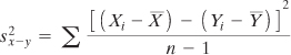
Earlier, this chapter noted that the basic theory of t-tests assumes that the populations from which the groups are sampled have the same variance. The procedure that follows from the assumption of equal variances is that two variances, one from each sample, are pooled to arrive at an estimate of the population variance. That pooling is done as shown in cells F1:F2 of Figure 9.1 and as repeated here in definitional form:

That discussion went on to point out that both theoretical and empirical research have shown that when the two samples have the same number of observations, violating the equal variances assumption makes a negligible difference to the outcome of the t-test.

In turn, that finding implies that you don’t worry about unequal variances when you’re running a dependent groups t-test. By definition, the two groups have the same sample size, because each member of one group must be paired with exactly one member of the other group.

That leaves the cases in which group sizes are different and so are their variances. When the larger group has the larger sample variance, it contributes a greater share of greater variability to the pooled estimate of population variance than does the smaller group.

As a result, the standard error of the mean difference is inflated. That standard error is the denominator in the t-test, and therefore the t-ratio is reduced. You are working with an actual alpha rate that is less than the nominal alpha rate, and statisticians refer to your t-test as conservative. The probability that you will reject a true null hypothesis is lower than you think.

But if the larger group has the smaller sample variance, it contributes a greater share of lower variability than does the smaller group. This reduces the size of the standard error, inflates the value of the t-ratio, and in consequence you are working with an actual alpha that is larger than the nominal alpha. Statisticians would say that your t-test is liberal. The probability that you will reject a true null hypothesis is greater than you think.

The Data Analysis Add-in Equal Variances t-Test

This tool is the classic t-test, largely as it was originally devised in the early part of the twentieth century. It maintains the assumption that the population variances are equal, it’s capable of dealing with groups of different sample sizes, and it assumes that the observations are independent of one another (thus, it does not calculate and use a correlation).

To run the equal variances tool (or the unequal variances tool or the paired sample, dependent groups tool), you must have the Data Analysis add-in installed, as described in Chapter 4. Once the add-in is installed, you can find it in the Analysis group on the Ribbon’s Data tab.

To run the Equal Variances t-test, activate a worksheet with the data from your two groups, as in columns B and C in Figure 9.8, and then click the Data Analysis button in the Analysis group. You will see a list box with the names of the available data analysis tools. Scroll down until you see “t-Test: Two-Sample Assuming Equal Variances.” Click it and then click OK. The dialog box shown in Figure 9.9 appears.

Figure 9.9. The t-test tools always subtract Variable 2 from Variable 1 when calculating the t-statistic.

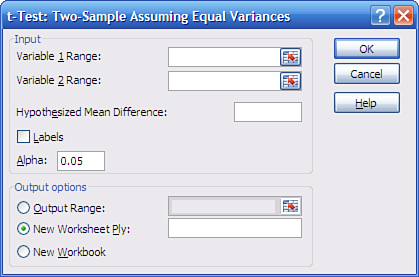
Here are a few comments regarding the dialog box in Figure 9.9 (which also apply to the dialog boxes that appear if you choose the unequal variances t-test or the paired sample t-test):

• As noted, Variable 2 is always subtracted from Variable 1. If you don’t want to get caught up in the very minor logical complications of negative t-statistics, make it a rule to designate the group with the larger mean as Variable 1. So doing is not the same as changing a nondirectional hypothesis to a directional one after you’ve seen the data. You are not altering your decision rule after the fact; you are simply deciding that you prefer to work with positive rather than negative t-statistics.

• If you include column headers in your data ranges, fill the Labels check box to use those headers instead of “Variable 1” and “Variable 2” in the output.

• The caution regarding the Output Range, made in Chapter 4, holds for the t-test dialog boxes. When you choose that option button, Excel immediately activates the address box for Variable 1. Be sure to make Output Range’s associated edit box active before you click in the cell where you want the output to start.

• Leaving the Hypothesized Mean Difference box blank is the same as setting it to zero. If you enter a number such as 5, you are changing the null hypothesis from “Mean 1 − Mean 2 = 0” to “Mean 1 − Mean 2 = 5.” In that case, be sure that you’ve thought through the issues regarding directional hypotheses discussed previously in this chapter.

After making your choices in the dialog box, click OK. You will see the analysis shown in cells E1:G14 in Figure 9.10.

Figure 9.10. Note that the Paired test in columns I:K provides a more sensitive test than the Equal Variances test in columns E:G.

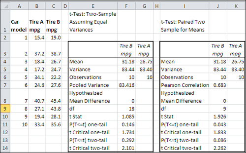
There are several points to note in the Equal Variances analysis in E1:G14 in Figure 9.10, particularly in comparison to the Paired Sample (dependent groups) analysis in I1:K14:

Compare the calculated t-statistic in F10 with that in J10. The analysis in E1:G14 assumes that the two groups are independent of one another. Therefore, the analysis does not compute a correlation coefficient, as is done in the “paired sample” analysis. In turn, the denominator of the t-statistic is not reduced by a figure that depends in part on the correlation between the observations in the two groups.

As a result, the t-statistic in F10 is smaller than the one in J10: small enough that it does not exceed the critical value needed to reject the null hypothesis at the .05 level of alpha either for a directional test (cell F11) or a nondirectional test (cell F13).

Also compare the degrees of freedom for the two tests. The Equal Variances test uses 18 degrees of freedom: ten from each group, less two for the means of the two groups. The Paired Sample test uses nine degrees of freedom: ten pairs of observations, less one for the mean of the differences between the pairs.

As a result, the Paired Sample t-test has a larger critical value. If the experimenter is using a directional hypothesis, the critical value is 1.734 for the Equal Variances test and 1.833 for the Paired Sample test. The pattern is similar for a nondirectional test: 2.101 versus 2.262. This difference in critical values is due to the difference in degrees of freedom: Other things being equal, a t-distribution with a smaller number of degrees of freedom requires a larger critical value.

But even though the Paired Sample test requires a larger critical value, because fewer degrees of freedom are available, it is still more powerful than the Equal Variances test because the correlation between the two groups results in a smaller denominator for the t-statistic. The weaker the correlation, however, the smaller the increase in power. You can convince yourself of this by reviewing the formula for the standard error of the difference between two means for the dependent groups t-test. See the section earlier in this chapter titled “Calculating the Standard Error for Dependent Groups.”

The Data Analysis Add-in Unequal Variances t-Test

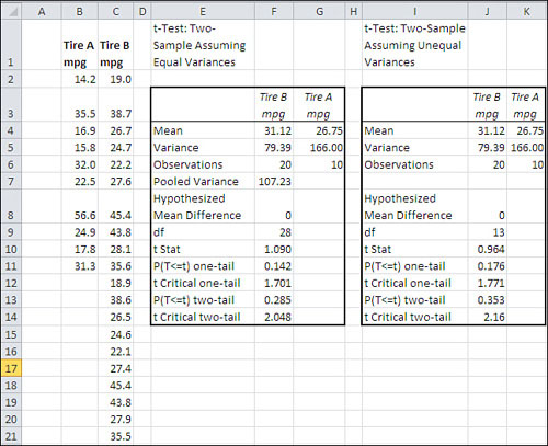
Figure 9.11 shows a comparison between the results of the Data Analysis add-in’s Equal Variances test and the Unequal Variances test.

Figure 9.11. The data has been set up to return a liberal t-test.

It is usual to assume equal variances in the t-test’s two groups if their sample sizes are equal. But what if they are unequal? The possible outcomes are as follows:

• If the group with the larger sample size has the larger variance, your alpha level is smaller than you think. If the nominal alpha rate that you have chosen is 0.05, for example, the actual error rate might be 0.03. You will reject the null hypothesis less often than you should. Thus, the t-test is conservative. (The corollary is that statistical power is lower than is apparent.)

• If the group with the larger sample size has the smaller variance, your alpha level is greater than you think. If the nominal alpha rate that you have chosen is 0.05, for example, the actual error rate might be 0.08. You will more often erroneously conclude a difference exists in the population where it doesn’t. The t-test is liberal, and the corollary is that statistical power is greater than you would expect.

Accordingly, the raw data in columns B and C in Figure 9.11 includes the following:

• The Tire B group, which has 20 records, has a variance of 79.

• The Tire A group, which has 10 records, has a variance of 166.

So the larger group has the smaller variance, which means that the t-test operates liberally—the actual alpha is larger than the nominal alpha and the test’s statistical power is increased.

However, even with that added power, the Equal Variances t-test does not report a t-statistic that is greater than the critical value, for either a directional or a nondirectional hypothesis.

The main point to notice in Figure 9.11 is the difference in degrees of freedom between the Equal Variances test shown in cells E1:G14 and the Unequal Variances test in cells I1:K14. The degrees of freedom in cell F9 is 28, as you would expect. Twenty records in one group plus ten records in the other group, less two for the group means, results in 28 degrees of freedom. However, the degrees of freedom for the Unequal Variances test in cell J9 is 13, which appears to bear no relationship to the number of records in the two groups. Also note that the t-statistic itself is different: 1.090 in F10 versus 0.964 in cell J10.

The Unequal Variances test uses what’s called Welch’s correction, so as to adjust for the liberal (or conservative) effect of a larger group with a smaller (or larger) variance. The correction procedure involves two steps:

1. For the t-statistic’s denominator, use the square root of the sum of the two variances, rather than the standard error of the mean difference.
2. Adjust the degrees of freedom in a direction that makes a liberal test more conservative, or a conservative test more liberal.

The specifics of the adjustment to the degrees of freedom are not conceptually illuminating, so they are skipped here; it’s enough to state that the adjustment depends on the ratios of the groups’ variances to their associated number of records.

For example, the data in Figure 9.11 involves a larger group with a smaller variance, so you expect the normal t-test to be liberal, with a higher actual alpha than the nominal alpha selected by the experimenter.

When Welch’s correction is applied, the t-Test for Unequal Variances uses 13 degrees of freedom rather than 28. As the prior section noted, a t-distribution with fewer degrees of freedom has a larger critical value for cutting off an alpha area than does one with more degrees of freedom.

Accordingly, the Unequal Variances test with 13 degrees of freedom needs a critical value of 1.771 to cut off 5% of the upper tail of the distribution (cell J12). The Equal Variances test, which uses 28 degrees of freedom, cuts off 5% of the distribution at the lower critical value of 1.701 (cell F12). This is because the t-distribution is slightly leptokurtic, with thicker tails in the distributions with fewer degrees of freedom.

Visualizing Statistical Power

Both Chapter 8 and this chapter have had much to say regarding statistical power. Several factors can influence how sensitive a t-test is to experimental data: the size of the treatment effect, the sample sizes, the standard deviation of the outcome measure, the size of alpha, and the directionality of the hypotheses.

Those factors all act together to influence power. Figure 9.12 shows a worksheet that can help you visualize the effects of those factors.

Figure 9.12. The spinners enable you to increase or decrease their associated values.

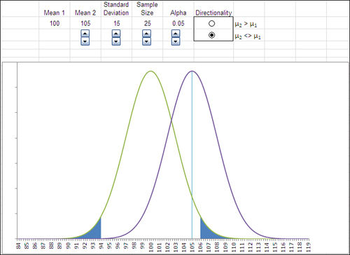
You can find the worksheet shown in Figure 9.12 in the workbook for Chapter 9 that is available on the book’s website at www.informit.com/title/9780789747204.

Use it to increase or decrease the treatment effect, change sample sizes (and therefore standard errors), standard deviations (and therefore standard errors, again), and so on. When you do so, the chart redraws to show the result of the change you made.

Watch in particular what happens in the right curve that represents the experimental group. The power of the t-test, as these curves are laid out, is the area under the right curve that lies to the right of the critical value that bounds the alpha area (shown in the right tail of the left distribution).

For example, if you reduce the treatment effect by reducing Mean 2, the right curve is pulled to the left and less of it lies to the right of the critical value. Power is reduced.

Alternatively, if you decrease the size of the standard deviation, the size of the standard errors decreases. That pulls the alpha area to the left, leaving more of the area of the right curve to the right of the critical value.

When to Avoid t-Tests

The theoretical underpinnings of t-tests do not account for more than two groups. The examples in Chapters 8 and 9 have all involved an experimental group and a control group. Although this is a typical design for good experiments, it is somewhat restrictive. There are many interesting questions whose answers require the use of three or more groups: for example, a drug trial involving a group that takes a new drug, a group that takes an existing drug or a placebo, and a group that takes no medication at all.

For this sort of situation, t-tests are not appropriate. Chapter 10, “Testing Differences Between Means: The Analysis of Variance,” explains why that is so, and introduces the statistical test that is designed to handle three or more groups: the analysis of variance.