Our work is the presentation of our capabilities.
—Edward Gibbon
The debate over the true definition of quality is as strong as ever with no resolution in sight.1 For the purposes of our discussion of process capability, we will use a definition based on Juran’s fitness for use and Feigenbaum’s best for certain customer conditions.2 Edward Lawson built on Juran’s and Feigenbaum’s work when he crafted his definition of quality as “the degree of excellence with which a product or service fulfills its intended purpose.”3 The intended purpose is defined by the marketplace, according to Lawson, and the intended purpose is translated into specifications that manufacturers use to assure the products they produce meet the customers’ intended purpose—that is, they are of good quality. As John Guaspari put it, “Customers aren’t interested in our specs. They’re interested in the answer to one simple question, “Did the product do what I expected it to do?”4
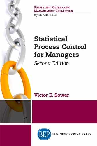
Process capability assesses how well the process, when operating in control, is able to meet the specifications. Process capability is important because simply being in control is not sufficient. A process that consistently produces nonconforming product can still be in control. Figure 7.1 illustrates a process operating in control with little variation but that fails to produce products that meet specifications because the process is not centered on the specification.
Figure 7.2 illustrates a process operating in control and that is centered on the specification that produces considerable amounts of nonconforming material because the process limits are too wide—that is, there is too much variation. While the control charts (not shown) for both illustrated processes indicate they are in control, neither of the processes shown in Figures 7.1 and 7.2 are capable since so much of the distribution is outside the specification limits. What is desired is a process that is both in control and capable.

Figure 7.1 In control, but not capable (A)
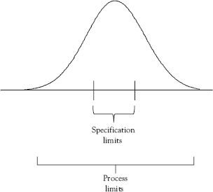
Figure 7.2 In control, but not capable (B)
Measurement of process capability differs for variable and attribute data. For that reason, we will deal with each separately.
Process Capability for Variable Data
There are several ways to measure process capability for variable data that we will discuss in this chapter. Among these are the process capability indices Cp, Cpk, and Cpm. These indices compare specifications for a product (what you desire the process to produce) to the process’s performance capability (what the process can achieve when operating in control). Regardless of which of these statistical indices is used, the first step in assessing process capability is to confirm that the specifications accurately reflect the customers’ intended purpose. The second step is to confirm that the process is in control. The third step is to compare the spread of the specifications to the variation of the in-control process. using some form of an index.
When the process is not in control, some experts recommend using the indices Pp and Ppk (known as process performance indices) to obtain an initial measure of process capability before the process is brought into a state of statistical control. However, if the process is not in control, these indices have no predictive capability because the process is not predictable. Indeed many experts5 regard the use of Pp and Ppk as a “step backward in quantifying process capability.” One expert6 flatly states that Pp and Ppk “are a waste of engineering and management effort—they tell you nothing.” Therefore, it is recommended that the process first be brought into a state of control, then use Cp, Cpk, or Cpm as measures of process capability rather than using Pp or Ppk.
Because all of these indices are a ratio of the spread of the specifications (distance between the upper and lower specification limits) and the variation in the process (±3σx), it is obvious that only two actions can increase the value of the ratio: increase the spread of the specifications or decrease the process variation.
The higher the value of the index the more capable is the process. Standards for considering a process to be capable sometimes differ from industry to industry and organization to organization. A general rule is that a Cp index value of 1.33 is a minimum acceptable standard for capability. As Table 7.1 shows, this corresponds to 63 parts per million defective (ppmd), assuming a perfectly normal distribution, which is a 4 sigma level of quality (See Table 7.1 footnote). In this context, 4 sigma refers to the upper specification limit (USL) and lower specification limit (LSL) coinciding with ±4 standard deviations from the process mean—a total spread of 8 standard deviations. The larger the value of the capability ratio, the larger the magnitude of an assignable cause event that can be tolerated without generating large amounts of out-of-specification material.
Table 7.1 Cp and ppm defective
Quality level |
Cp |
ppm defective |
3 sigma |
1.00 |
2,700 |
4 sigma |
1.33 |
63 |
5 sigma |
1.67 |
0.57 |
6 sigma* |
2.00 |
0.002 |
Source: Sower (2011); Adapted from Tadikamalla (1994).
*The Six Sigma quality program allows the distribution mean to drift by ± 1.5 standard deviations. Six sigma quality without the drift equates to 0.002 ppm defective. Six Sigma quality with the drift allowed equates to the often quoted 3.4 ppm defective or 3.4 defective parts per million opportunities.
When the process is centered on the target value of the specification (T), there are only two actions that can be taken to improve process capability as shown in Figure 7.3:
• Decrease process variation
• Loosen the specification
If the process is not centered on the process specification, process capability can also be improved by centering the process on the specification (see Figure 7.6).
The equations for calculating the measures of process capability discussed in this section may be found in Table A.4 in Appendix A.
Example 7.1
Why Isn’t Cp = 1.00 Good Enough?
A manufacturer of electronic toys aspired for a process that is in control with a Cp of 1.00. “After all, we’re not producing space shuttles. I don’t think that 2,700 defective toys out of every million produced is so bad. That is only about 1 defective product out of every 400 units produced, which means that 99.73 percent or our products work properly. We will just replace the defective ones that are returned by the customer.”
But assume that her toys are comprised of 100 components each produced by processes that are in control and have a Cp = 1.00. If any one of these components fails to work properly, the toy will fail to work. Each component has a probability of working properly of 0.9973. The probability of all of the components working properly is 0.9973 × 0.9973 × 0.9973 … 100 times or 0.9973100. The resulting reliability is 0.7631. That means that about 24 out of each 100 products produced will be defective. This is hardly acceptable even for toys. A higher standard is needed. At the minimum accepted standard Cp = 1.33, the reliability of the toy would still be just 0.8591, resulting in about 14 defective toys per 100 produced.

Figure 7.3 Improving process capability
Cp is defined by ASQ as the “ratio of tolerance to 6 sigma, or the USL minus the LSL divided by 6 sigma. It is sometimes referred to as the engineering tolerance divided by the natural tolerance.”7 This definition uses the term tolerance while this book uses the term specification to mean the same thing. Note also that in this definition, 6 sigma refers to a total spread of 6 standard deviations—3 standard deviations below the mean plus 3 standard deviations above the mean. This does not have the same meaning as Six Sigma referring to the quality program used by some organizations to reduce process variation.
Cp is an appropriate measure of process capability when:
• The specification is two sided—that is it has both an upper and a lower bound.
• The process is centered on the specification target value (see Figure 7.2).
• The individual measurements of process output are approximately normally distributed.
• The process is in control.
Statistical process control (SPC) uses statistics derived from both samples and individuals. It is important to understand when to use each. This is especially true when dealing with x-bar charts and process capability analysis. Data are collected for the construction of x-bar charts using rational subgroups (see Chapter 4) or samples consisting of two or more observations. The sample means ![]() are calculated along with the sample ranges (R) or sample standard deviations (s). The mean of the sample means is the grand mean
are calculated along with the sample ranges (R) or sample standard deviations (s). The mean of the sample means is the grand mean ![]() the mean of the sample ranges is
the mean of the sample ranges is ![]() and the standard deviation of the sample means is
and the standard deviation of the sample means is ![]() These statistics are used to determine the UCL and LCL for the x-bar chart upon which the sample means are plotted.
These statistics are used to determine the UCL and LCL for the x-bar chart upon which the sample means are plotted.
Usually these same data are used to determine a measure of process capability such as Cp or Cpk, but for process capability purposes, it is the individual measurements rather than the sample statistics that are used. So, when calculating process capability, we use the standard deviation of the individual measurements (σx). For more detail about this topic, see Appendix A.
Example 7.2
Using the Same Data for an X-Bar Chart and Process Capability
Part weight data were collected from a molding operation for the purpose of implementing SPC for the process. Twenty-five samples consisting of four parts each were collected from the process as shown in Table 7.2.
Table 7.2 Sample data
Sample no. |
Part 1 |
Part 2 |
Part 3 |
Part 4 |
1 |
19.97 |
20.03 |
20.05 |
20.10 |
2 |
19.97 |
19.96 |
19.99 |
20.00 |
3 |
20.06 |
19.99 |
20.03 |
20.10 |
4 |
20.00 |
20.02 |
20.01 |
19.94 |
5 |
20.08 |
20.00 |
19.84 |
20.08 |
6 |
20.01 |
19.98 |
19.92 |
20.03 |
7 |
20.03 |
20.06 |
20.00 |
19.98 |
8 |
20.03 |
20.02 |
20.00 |
20.08 |
9 |
19.94 |
20.02 |
19.96 |
19.89 |
10 |
19.92 |
19.95 |
20.05 |
20.06 |
11 |
20.01 |
19.98 |
20.02 |
19.88 |
12 |
19.90 |
20.00 |
19.95 |
20.09 |
13 |
19.97 |
20.03 |
20.05 |
20.10 |
14 |
19.97 |
19.96 |
19.99 |
20.00 |
15 |
20.06 |
19.99 |
20.03 |
19.92 |
16 |
20.03 |
20.02 |
20.01 |
19.94 |
17 |
20.08 |
20.00 |
20.08 |
20.08 |
18 |
20.01 |
19.98 |
19.92 |
20.03 |
19 |
20.03 |
20.00 |
20.00 |
19.94 |
20 |
20.03 |
20.04 |
20.00 |
19.94 |
21 |
19.94 |
20.02 |
19.96 |
19.89 |
22 |
19.98 |
19.95 |
20.02 |
20.06 |
23 |
20.01 |
19.98 |
19.96 |
20.06 |
24 |
20.00 |
20.11 |
19.95 |
20.09 |
25 |
19.97 |
19.98 |
19.99 |
20.00 |
First, the sample means and sample ranges were calculated by the SPC software package and used to construct x-bar and R-charts. Figure 7.4a shows that the process is in control. Next, the individual observations were analyzed and the process mean and standard deviation were calculated and used to analyze process capability. Figure 7.4b shows that the process distribution is approximately normal and reasonably centered on the specification target. The organization uses a standard of Cp at or above 1.33 to classify a process as being capable. Using this standard, the process is capable since Figure 7.4b indicates Cp is 1.5458.

Figure 7.4 State of control and capability analysis using data in Table 7.2
Source: Created using NWA Quality Analyst 6.3.
Figure 7.4b shows a typical process capability report. From this report, we can see that the process distribution is approximately normal and the process mean almost exactly coincides with the target value of the specification. On the printout, samples = 100 indicates that 4 observations from each of the 25 samples were used in this analysis (4 observations per sample × 25 samples = 100 individual observations). Three process capability indices are reported: Cp, Cpk, and Cpm. The final entry on the printout (Est.% out) shows that over time, approximately 0.0002 percent of the process output is expected to fall below the LSL and 0.0002 percent is expected to fall above the USL for a total prediction of a long-term average of 0.0004 percent of the output failing to meet specifications.
Cpk
When the second requirement for using Cp, “the process mean is centered on the specification target” (see Figure 7.1), is not met, then the proper index to use is Cpk. Think of Cpk imposing a penalty on process capability if the process is not centered on the specification target value. Cpk separately examines the distance between the USL and the process mean and the distance between the LSL and the process mean. It calculates two ratios: (1) the ratio of distance between the process mean and the LSL to 3 sigma and (2) the ratio of the distance between the USL and the process mean to 3 sigma. The former ratio is referred to as Cpl and the latter as Cpu. Cpk is the minimum of these two ratios.
Figure 7.5 illustrates a situation where the specification target value is higher than the process mean (µ)—that is, the process mean is not centered on the target value. The distance between the LSL and the process mean is smaller than the distance between the process mean and the USL. Since each distance is divided by the same value, 3 sigma, that means Cpl will be smaller than Cpu and Cpk would be set at the value of the Cpl. As with Cp, the higher the value of the Cpk the more capable is the process. The general rule is that a Cpk value of 1.33 is a minimum acceptable standard for capability although many organizations adopt a different value of the index for their purposes.
When the process is perfectly centered on the specification target value, Cp and Cpk will be identical. For un-centered processes, centering the process on the specification target value will increase process capability. Note in the process capability printout in Figure 7.4b, the process is not exactly centered on the process mean. We can tell that because Cp is 1.5458 while Cpk is 1.5377—close but not identical. We would use Cpk as the current capability of this process while the difference between Cp and Cpk represents the amount of improvement that could be achieved by perfectly centering the process on the target value. Often shifting the process mean to more closely align with the specification target value is easier to accomplish than reducing process variation. For this reason, shifting the mean so that it more closely coincides with the specification target value should not be overlooked as a possible source of process improvement as shown in Figure 7.6.
Figure 7.5 Cpk, Cpl, and Cpu—Process not centered on target value

Figure 7.6 Process improvement through shifting of the mean
Cpm
Cpk exacts a penalty for the process not being centered on the specification target value, but the value of this penalty is small if the process variation is small enough so that the amount of out-of-specification product produced is small. Cpm is an index that is based on the Taguchi loss function, which, in part, states that there is a loss to society when a process mean is off target (ideal value) even if no out-of-specification product is produced.8,9 Some consider Cpm to be the best overall “indicator of how your customers experience the quality of your product or service.”10
While Cp and Cpk use the process mean when calculating the spread of the observations, Cpm uses the specification target value instead and compares this spread with the distance between the USL and LSL. In the left-hand illustration in Figure 7.6, the process is so far off target that it is obvious that significant amounts of out-of-specification product will be produced. Cpk penalizes for this. Figure 7.7 illustrates the situation where the process is not centered, but the variation is small enough that little out-of-specification product is produced. Cpm penalizes more than Cpk in this situation. Most SPC software reports Cpm as well as Cp and Cpk as part of its process capability analysis routine (see Figure 7.4b).
Process Capability for Variables Data—One-Sided Specification Limit
The previous discussions dealt with the situation where specifications are two-sided—that is target value ± some value representing the USL and LSL, which is sometimes expressed as from LSL to USL. There are many situations where the specification is one-sided—that is target + 0/–0.002 or not to exceed USL where 0 is ideal. In these cases, the target value is not midway between the LSL and USL. The target value is the LSL. In this case, process capability is measured using Cpu or in more precise terms, we measure process capability using Cpk where Cpk = Cpu. The assumption of normality in the process data must still be satisfied.
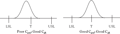
Figure 7.7 Improving Cpm through process centering
Example 7.3
Process Capability for One-Sided Specifications
The Environmental Protection Agency maximum concentration level for arsenic in potable water is 0.010 ppm.11 The ideal or goal is 0 ppm arsenic in the water. This is a situation where the target value is the LSL (0 ppm).
A bottling company extracts water from a well which is then filtered, sanitized using UV radiation, and bottled for sale. Samples from the bottling line are taken periodically and tested for a variety of potential contaminants. Among the tests is one to determine the amount of arsenic present in the water. The process is in control and the distribution of the individual observations is approximately normal. The appropriate measure of process capability for this process would be Cpk = Cpu. Because this is a critical statistic, the company uses a standard of Cpk ≥ 2.00 as their measure of process capability. The measured value of Cpk is 2.05, which is above the standard, therefore the process is considered to be capable.
Process Capability for Nonnormal Distributions
The use of Cp, Cpk, and Cpm require that the process distribution is approximately normal. There are many situations where this might not be the case. It is possible to accommodate nonnormal distributions by identifying the appropriate distribution and selecting it for use when determining process capability. Figure 7.10 shows the process capability parameter selection screen for NWA Quality Analyst.
Example 7.4
Process Capability with Nonnormal Distribution
A manufacturing company tracks the time it takes to prepare shipments from its factory. They use day as the rational subgroup and x-bar and s-charts with variable sample sizes to determine the state of control of the process. The control charts indicate the process is in control. The company has set a goal of 5 minutes per shipment and an upper bound of 10 minutes per shipment and wants to understand the process’s capability to meet these specifications.
Their first attempt to assess process capability used the software’s default setting of the normal distribution to model their process. The output they obtained is in Figure 7.8.
By visual examination, we can see that the data do not fit the normal distribution, which renders Cpk meaningless. The shape of the distribution suggests instead a Weibull12 distribution.13 Note that there are statistical tests to determine how well data fit a specific distribution, but for the purpose of this book, we will rely on visual examination. They make the appropriate selection in NWA Quality Analyst (see Figure 7.10) and obtain Figure 7.9.
Visually, the Weibull distribution is a much better fit for the data. The printout shows that Cpk = 0.9988 while the company was targeting a Cpk = 1.33 as their minimum standard. They conclude the process is not capable as currently designed and initiate an improvement project to increase the capability of the process.

Figure 7.8 Package preparation times modeled using the normal distribution
Source: Created using NWA Quality Analyst 6.3.

Figure 7.9 Package preparation times modeled using the Weibull distribution
Source: Created using NWA Quality Analyst 6.3.
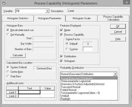
Figure 7.10 Probability distributions available for process capability analysis in NWA Quality Analyst 6.3
Process Capability for Attributes Data
Process capability for attributes data is less complex than for variables data. One measure of process capability is the centerline value of the attribute control charts. This works well for p-charts and u-charts, but less well for np-charts and c-charts. To say that a process is capable of producing on average a ![]() = 0.002 has meaning as a standalone measure and can be used as a predictor. We would expect the process, if it remains in control, to continue to produce an average proportion defective of 0.002. Similarly, a
= 0.002 has meaning as a standalone measure and can be used as a predictor. We would expect the process, if it remains in control, to continue to produce an average proportion defective of 0.002. Similarly, a ![]() = 0.10 also has meaning as a standalone measure. We would expect the process, if it remains in control, to continue to produce an average of 0.10 defects per unit.
= 0.10 also has meaning as a standalone measure. We would expect the process, if it remains in control, to continue to produce an average of 0.10 defects per unit.
Neither ![]() (the central line for the np-chart) nor c (the central line for the c chart) work as well as standalone measures of process capability. The sample size must be included in order for these measures of process capability to be meaningful. The number of defective units in a sample and the number of defects in a sample must have the sample size specified in order to be meaningful. This is cumbersome.
(the central line for the np-chart) nor c (the central line for the c chart) work as well as standalone measures of process capability. The sample size must be included in order for these measures of process capability to be meaningful. The number of defective units in a sample and the number of defects in a sample must have the sample size specified in order to be meaningful. This is cumbersome.
Another popular approach to measuring process capability with attribute data is to use the measure “parts per million defective” sometimes known as the number of defectives per million opportunities. The abbreviations parts per million (ppm), defects per million opportunities (DPMO), and parts per million defective (ppmd) are variously used with this measure. This is a popular measure in the Six Sigma approach to quality.
Another popular approach involves the use of sigma notation. As Table 7.1 showed, there is a relationship between ppm and the number of standard deviations defining the spread of the specification limits relative to the spread of the process distribution. Three sigma quality coincides to 2,700 ppmd for example. However, care must be taken when using this approach. The Six Sigma quality program allows a ±1.5σ shift in the process mean when calculating this quality measure. Allowing for this shift, 3σ quality now coincides with 65,000 ppmd instead of 2,700. The Six Sigma program goal of making all processes Six Sigma capable is defined as 3.4 ppmd when the 1.5σ shift is allowed, but 0.002 ppmd when the mean is not allowed to shift.
Regardless of the measure, the organization must determine the process capability necessary to delight its customers. For some 2,700 ppmd is sufficient; for others, this would represent dreadful performance. Setting the process capability goal is a management responsibility.
Chapter Take-Aways
When a process is centered on the specification target value, there are only two actions that can improve process capability:
• Decrease process variation
• Loosen the specification
When the process is not centered on the specification target value, centering the process can improve process capability.
The process for using process capability indices Cp, Cpk, and Cpm is:
• Confirm that the specifications accurately reflect the customers’ intended purpose.
• Confirm that the process is in control.
• Verify that distribution of individual measurements is approximately normal (or identify and use the appropriate alternative distribution). This should be done using statistical measures of goodness of fit.
• Compare the spread of the specifications to the variation of the in-control process using the appropriate index.
• Determine whether the process capability index meets expectations (e.g., Cp = 1.33 or Cp = 2.00).
The larger the value of the capability ratio, the larger the magnitude of an unexpected event that can be tolerated without generating large amounts of out-of-specification material.
The goals of process capability are:
• To have all of the variable process indices equal to each other (Cp = Cpk = Cpm), indicating the process is centered on the specification target value, and
• Greater than the organization’s standard for considering a process to be capable (e.g., 1.33 or 2.00).
Modern SPC software allows for the easy analysis of process capability for processes that are not normally distributed.
Process capability using attributes data is usually defined in terms of average proportion defective, average number of defects per unit, parts per million defective, or the number of standard deviations defining the spread of the specification limits relative to the spread of the process distribution.
Process capability is useful in predicting the performance of processes and customer satisfaction with the output of those processes. However, the goals for process capability must be set by management to achieve the level of performance demanded by customers.
Questions You Should be Asking About Your Work Environment
• How well do the specifications for your products and services reflect customer requirements?
• How many of your processes have established levels of process capability?
• Are all of your processes properly centered on the target value?
• Have you established the level of process capability necessary to meet customer requirements?
• Is improving process capability an integral part of your continuous quality improvement program?
• What gains would accrue to your organization from increasing process capability?