
8
Inference in Parametric and Semi-parametric Models: The Divergence-based Approach
This chapter presents a short review of basic features of statistical inference in parametric and semi-parametric models through duality techniques in the realm of divergence-based methods. A simple solution for testing the number of components in a mixture is presented; this is a non-regular model with currently no amenable solution. The interplay between the choice of the divergence and the model is enlightened.
8.1. Introduction
This paper aims to present the main features of Csiszár-type divergences in relation with statistical inference. We first introduce some notations and definitions, and then embed the present setup in the context of decomposable measures of discrepancy between probability measures. A variational representation of Csiszár divergences is the basic ingredient for this embedding. The specificity of the classes of decomposable measures of discrepancy allows us to select such a class for specific inference purposes.
Minimizing a discrepancy between a given distribution P and a class of measures M occurs in a certain number of problems. On the one hand, when the distribution P is known, then the resulting problem is of analytic nature and bears no statistical aspect. On the other hand, the measure P might only be known through a sampling of observations X1, .., Xn, whose empirical distribution
converges to P in some sense. The class M is then called a model, which may be parametric, therefore indexed by some θ in a subset Θ of a finite dimensional space; the model M might be semi-parametric, for example described by moment or L-moment conditions; or non-parametric, for example when described by shape conditions, such as unimodality. Inference in those cases aims at answering basic questions:
Does P belong to M?
If yes, and when the model is of parametric or semi-parametric nature, what is the “true” value θT of the parameter for which P = PθT, a question which should obviously be made more precise according to the context; for example, in semi-parametric models, the class M is usually described as
where Mθ represents a whole submodel sharing a common feature θ, and the inference estimation step aims at identifying θT such that P belongs to MθT. The case when each of the Mθ is defined by specific moment conditions extends the classical empirical likelihood context and will be described in section 8.2. Other fields of application of a minimum divergence approach cover robust inference in parametric models, considering minimum divergence estimation between the distribution of the data and some tubular neighborhoods of the model. Model selection criteria such as AIC or BIC can be considered as minimum divergence estimators. Broadly speaking, divergence-based methods extend the likelihood paradigm in a natural way, paving the way to trade-off between efficiency and robustness requirements. In this chapter, we will show the way in which some non-regular problems can be solved accordingly, in the realm of mixture models.
We now turn to some definitions and notations.
8.1.1. Csiszár divergences, variational form
8.1.1.1. Parametric framework
Let P := {Pθ,θ ∈ Θ} be an identifiable parametric model on ℝd, where Θ is a subset of ℝs. All measures in P will be assumed to be measure equivalent, therefore sharing the same support. The parameter space Θ does not need to be an open set in the present setting. It may even happen that the model includes measures which would not be probability distributions; cases of interest cover models including mixtures of probability distributions; this will be developed in section 8.3. Let ϕ be a proper closed convex function from ] – ∞, +∞[ to [0, +∞] with ϕ(1) = 0 and such that its domain domϕ := {x ∈ ℝ such that ϕ(x) < ∞} is an interval with endpoints aϕ < 1 < bϕ(which may be finite or infinite). For two measures Pα and Pθ in P, the ϕ-divergence between Pα and Pθ is defined by
In a broader context, the ϕ-divergences were introduced by Csiszár (1964) as “f-divergences”, defined between two probability measures Q and P, with Q absolutely continuous (a.c.) with respect to (w.r.t.) P by
where f satisfies the same requirements as ϕ above. The basic property of ϕ-divergences states that when ϕ is strictly convex on a neighborhood of x = 1, then
We refer to (Liese and Vajda 1987, Chapter 1) for a complete study of those properties. Let us simply quote that in general φ(α, θ) and φ(θ, α) are not equal. Hence, ϕ-divergences usually are not distances, but they merely quantify some difference between two measures. A main feature of divergences between distributions of random variables X and Y is the invariance property with respect to a common smooth change of variables.
8.1.1.1.1. Examples of ϕ-divergences
The Kullback-Leibler (KL), modified Kullback-Leibler (KLm), χ2, modified χ2![]() , Hellinger (H) and L1 divergences are, respectively, associated with the convex functions ϕ(x) = x log x – x + 1, ϕ(x) = –log x + x –1,
, Hellinger (H) and L1 divergences are, respectively, associated with the convex functions ϕ(x) = x log x – x + 1, ϕ(x) = –log x + x –1, ![]()
![]() and ϕ(x) = |x – 1|. All of these divergences, except the L1, belong to the class of the so-called “power divergences” introduced in Read and Cressie (1988) (see also Liese and Vajda 1987, Chapter 2), a class that takes its origin from Rényi et al. (1961). They are defined through the class of convex functions
and ϕ(x) = |x – 1|. All of these divergences, except the L1, belong to the class of the so-called “power divergences” introduced in Read and Cressie (1988) (see also Liese and Vajda 1987, Chapter 2), a class that takes its origin from Rényi et al. (1961). They are defined through the class of convex functions
if γ ∈ ℝ {0,1}, ϕ0(x) := – log x + x – 1 and ϕ1(x) := x log x – x + 1. So, the KL-divergence is associated with ϕ1, the KLm to ϕ0, the χ2 to ϕ2, the ![]() to ϕ –1 and the Hellinger distance to ϕ1/2.
to ϕ –1 and the Hellinger distance to ϕ1/2.
It may be convenient to extend the definition of the power divergences in such a way that φ(α, θ) may be defined (possibly infinite) even when Pα or Pθ is not a probability measure. This is achieved setting
when domϕ = ℝ+/{0}. Note that, for the χ2-divergence, the corresponding ϕ function ![]() is defined and convex on whole R.
is defined and convex on whole R.
We will only consider divergences defined through differentiable functions ϕ, which we assume to satisfy the following condition:
| RC | There exists a positive δ such that, for all c in [1 – δ, 1 + δ], we can find numbers c1, c2, c3 such that ϕ(cx) ≤ c1 ϕ(x) + c2 |x| + c3, for all real x |
Condition (RC) holds for all power divergences including KL and KLm divergences.
8.1.2. Dual form of the divergence and dual estimators in parametric models
Let θ and θT be any parameters in Θ. We intend to provide a new expression for φ(θ,θT).
As will be considered in statistical applications pertaining to non-regular models, it may be of interest, at times, to consider enhanced statistical models indexed by the parameter θ, and those models may include signed measures, although, obviously, no dataset would be generated by those. In any case, PθT clearly will designate a probability measure, under which the data are supposed to be generated. In those cases, the domain of ϕ will be assumed to contain all possible real values for (dPθ/dPθT) (x), henceforth a (possibly infinite) interval in ℝ; the χ2 divergence function
is the prototype for those cases.
By strict convexity, for all a and b the domain of ϕ it holds
with equality if and only if a = b.
Let us denote ϕ# (x) := xϕ’(x) – ϕ(x). For any α in Θ, define ![]() and also define
and also define ![]() Inserting these values in [8.4] and integrating with respect to PθT yields
Inserting these values in [8.4] and integrating with respect to PθT yields
Assume at present that this entails
for suitable α’s in some set Fθ included in Θ.
When α = θT, the inequality in [8.5] turns to equality, which yields
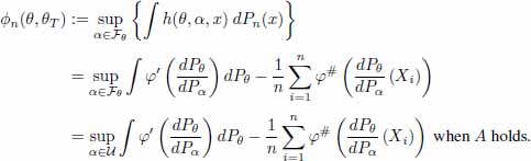
Denote
from which
Furthermore, by [8.5], for all α in Fθ

and the function x → h(θ, θT, x) = – h(θ, α, x) is non-negative due to [8.4]. It follows that φ(θ, θT) – ∫ h(θ, α,x)dPθT is zero if and only if (iff) h(θ,α,x) = h(θ, θT, x) – PθT a.e. Therefore, φ(θ, θT) – ∫ h(θ, α, x)dPθT = 0 iff for any x in the support of PθT,
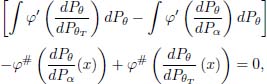
which cannot hold when the functions ![]() ,
,![]() and 1 are linearly independent, unless α = θT. We have proved that θT is the unique optimizer in [8.6].
and 1 are linearly independent, unless α = θT. We have proved that θT is the unique optimizer in [8.6].
We have skipped some sufficient conditions that ensure that [8.5] holds.
Assume that for all α in Fθ
Assume further that φ(θ, θT) is finite. Since

we obtain
which entails [8.5]. When ![]() , then clearly, under [8.9]
, then clearly, under [8.9]
We have proved that [8.6] holds when α satisfies [8.9].
Sufficient and simple conditions encompassing [8.9] can be assessed under standard requirements for nearly all divergences. We state the following result (see Liese and Vajda 1987; Broniatowski and Keziou 2006, lemma 3.2).
LEMMA 8.1.– Assume that RC holds and φ(θ, α) is finite. Then [8.9] holds.
Summing up, we can state the following result.
THEOREM 8.1.– Let θ belong to Θ and let φ(θ, θT) be finite. Assume that RC holds. Let Fθ be the subset of all α’s in Θ such that φ(θ, α) is finite. Then
Furthermore, the supremum is attained for θT and uniqueness holds true.
For the Cressie-Read family of divergences with γ ≠ 0,1, this representation writes

The set Fθ may depend on the choice of the parameter θ. Such is the case for the χ2 divergence, i.e. ϕ(x) = (x – 1)2/2, when pθ(x) = θ exp(–θx)1[0,∞)(x). In most cases, the difficulty of dealing with a specific set Fθ depending on θ can be encompassed when
there exists a neighbourhood U of θT for which [A]
which, for example, holds in the above case for any θT. This simplification deserves to be stated in the next result.
THEOREM 8.2.– When φ(θ, θT) is finite and RC holds, then, under condition [A],
Furthermore, the supremum is attained for θT and uniqueness holds true.
REMARK 8.1.– Identifying Fθ might be cumbersome. This difficulty also appears in the classical MLE case, a special case of the above statement with divergence function ϕ0, for which it is assumed that
is finite for θ in a neighborhood of θT.
Under the above notation and hypotheses, define
It then holds that Tθ (PθT) = θT for all θT in Θ. Also let
which also satisfies S(PθT) = θT for all θT in Θ. We thus can state the following result.
THEOREM 8.3.– When φ(θ, θT) is finite for all θ in Θ and RC holds, both functionals Tθ and S are Fisher consistent for all θT in Θ.
8.1.2.1. Plug in estimators
From [8.8], simple estimators for θT can be defined, plugging any convergent empirical measure in place of PθT and taking the infimum w.r.t. θ in the resulting estimator of φ(θ, θT).
In the context of simple i.i.d. sampling, introducing the empirical measure
where the Xi ’s are i.i.d. r.v’s with common unknown distribution PθT in P, the natural estimator of φ(θ, θT) is
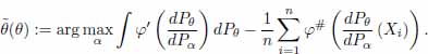
Denote by θ any given value in Θ and call it an escort parameter. Note that for any such θ, the supremum w.r.t. α in [8.10] is achieved at θT. A first M-estimator ![]() of θT with escort parameter θ can then be defined through
of θT with escort parameter θ can then be defined through
Those estimators coincide with the MLE for ϕ(x) = – log x + x = – 1 and they can be tuned through the choice of the escort parameter θ. Under condition A, since
the resulting estimator of φ(θT, θT) is
Also the estimator of θT is obtained as
In the case when ϕ = ϕγ defined by [8.2], it holds true
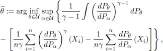
for γ ≠ 0,1. When γ = 0 the above expression [8.16] boils down to the classical expression
where μ is some dominating measure P. When γ = 1, then
The resulting minimum dual divergence estimators [8.15] and [8.16] do not require any smoothing or grouping, in contrast with the classical approach that involves quantization. The paper by Broniatowski and Keziou (2009) provides a complete study of those estimates and subsequent inference tools for the usual i.i.d. sample scheme. For all divergences considered here, these estimators are asymptotically efficient in the sense that they achieve the Cramer-Rao bound asymptotically in regular models. The case when ϕ = ϕ0 leads to θML defined as the celebrated maximum likelihood estimator (MLE), in the context of the simple sampling.
8.1.2.2. Dual form of the divergence and dual estimators in a general framework
The above derivation clearly leads to a similar description of
whenever Q is an a.c. measure w.r.t. P and φ (Q, P) = +∞ otherwise. Here, Q might be a signed measure and P is a probability measure; therefore, the domain of the convex function ϕ may at time overlap with the negative axis. The same development as above clearly yields for finite φ(Q, P)
where F designates any class of function that contains the function x → (dQ/dP)(x), since indeed the supremum in the RHS of the above display holds when f = (dQ/dP) (x) – Pa.e. Integrability condition for this representation to hold can be written
for all f in F, in accordance with [8.9].
Formula [8.17] is of relevance when Q belongs to some class of distributions for which (dQ/dP) (x) has a known functional form; such is the case in many semi-parametric settings, for example for models M defined through moment conditions, or in odd ratio models (see Broniatowski and Keziou 2012; Keziou and Leoni-Aubin 2008) for which the functional form of the likelihood ratio between the true unknown distribution P and the measures in the model is indeed a specification of the model; the resulting plug in estimator of the φ-projection Q* of P on M can be obtained through a similar procedure as in the parametric case
where X1, .., Xn are sampled under P.
8.1.3. Decomposable discrepancies
We now explore the relation between Csiszár discrepancies and statistical criteria; see Broniatowski and Vajda (2012) for additional insights. Turning back to the parametric setting, the φ-divergences ![]() can be embedded in the broader class of pseudodistances D, which are defined by the condition that
can be embedded in the broader class of pseudodistances D, which are defined by the condition that
An additional restriction imposed on pseudodistances D(P,Q) will be the decomposability property. In the sequel Q would designate a probability measure, which may be an atomic one (typically Q is the empirical measure Pn). Here, P designates the class of probability measures on some measurable set X.
A pseudodistance D is a decomposable pseudodistance if there exist functional D0 : P ↦ ℝ, D1 :P ↦ ℝ and measurable mappings
such that for all θ ∈ Θ and Q ∈ P the expectations ∫ ρθdQ exist and
We say that a functional TD : Q ↦ Θ defines a minimum pseudodistance estimator (briefly, min D-estimator) if D(Pθ,Q) is a decomposable pseudodistance and the parameters TD(Q) ∈ Θ minimize D0(Pθ) + ∫ ρθdQ on Θ, in symbols
In particular, for Q = Pn
Every min D-estimator θD,n is Fisher consistent in the sense that
Clearly, minimal φ-divergence estimators with escort θ, as defined in [8.14], are min D-estimators for the decomposable pseudodistance
and the maximum subdivergence estimator
with the divergence ϕ and escort parameter θ ∈ Θ is the min D-estimator for the decomposable pseudodistance.
8.1.3.1. Power pseudodistance estimators
A special class of pseudodistances Dψ (Pθ, Q) is defined on P ⊗ P by the integral
where ψ(s,t) are reflexive in the sense that they are non-negative functions of arguments s,t > 0 with ψ(s,t) = 0 iff s = t. If a function ψ is reflexive and also decomposable in the sense
for some ψ0,ψ1,ρ : (0, ∞) → ℝ, then the corresponding ψ-pseudodistance Dψ(Pθ,Q) is a decomposable pseudodistance satisfying
for
8.1.3.1.1. ϕ-divergences Dϕ(Pθ,Q)
The ϕ-divergences Dϕ,(Pθ, Q) are special ψ-pseudodistances for the functions
since they are non-negative and reflexive, and [8.19] implies Dψ(Pθ,Q) = Dϕ(Pθ,Q) for all P ∈ P,Q ∈ P when ϕ and ψ are related by [8.19]. However, the functions [8.19] in general do not satisfy the decomposability condition [8.18] so that the ϕ-divergences are not in general decomposable pseudodistances. An exception is the logarithmic function ϕ = ϕ0 = – log x + x – 1 for which the min Dϕ0 -estimator is the MLE.
8.1.3.1.2. L2-estimator
The quadratic function ψ(s,t) = (s – t)2 is reflexive and also decomposable. Thus, it defines the decomposable pseudodistance
on P ⊗ P. It is easy to verify that
The corresponding min Dψ-estimator is in this case the L2 -estimator
which is known to be robust but not efficient (see for example Hampel et al. 1988).
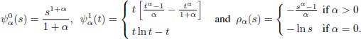
To build a smooth bridge between the robustness and efficiency, one needs to replace the reflexive and decomposable functions ψ by families {ψα : α ≥ 0} of reflexive functions decomposable in the sense
where the two functions ![]() and
and ![]() are defined at α = 0 through the limits
are defined at α = 0 through the limits
for some constant x all s > 0. Then for all α ≥ 0 and (Pθ,Q) ∈ P ⊗ P, the family of ψα-pseudodistances
satisfies the decomposability condition
for
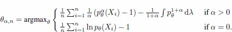
8.1.3.2. Dα estimators
The pseudodistances Dα(Pθ,Q) are decomposable and define the family of min Dα-estimators

This family contains as a special case for α = 0 the efficient but non-robust MLE
while for α > 0 the θα,n’s are expected to be less efficient but more robust than θ0,n.
Decomposable pseudodistances Dα(Pθ, Q) defined by the functions
of variables s, t > 0 where ϕ1+α and ϕα are the power functions defined through
Moreover, this family is continuous in the parameter α ↓ 0 and leads to MLE as its limit.
8.1.3.3. Relation with other estimation criteria
Let us call the pseudodistances Dα(P,Q) simply power distances of orders α ≥ 0.
8.1.3.3.1. L2-estimator revisited
The min Dα-estimator of order α = 1 is defined by
so that it is nothing but the L2-estimator θn. The family of estimators θn,α smoothly connects this robust estimator with the efficient MLE θn,0 when the parameter α decreases from 1 to 0.
The special class of the min Dα-estimators θα,n given above was proposed by Basu et al. (1998) who confirmed their efficiency for α ≈ 0 and their intuitively expected robustness for α > 0. These authors called θα,n minimum density power divergence estimators without actual clarification of the relation of the “density power divergences” Dα(P,Q) to the standard power divergences Dα(P, Q) studied in Liese and Vajda (1987) and Read and Cressie (1988).
This subclass of general min Dα-estimators [8.20] was included in a wider family of generalized MLE’s introduced and studied previously in Vajda (1984 and 1986).
8.1.3.4. Invariance
If the observations x ∈ χ are replaced by y = T(x), where T : (χ, A) ↦ (y,B) is a measurable statistic with the inverse T–1 then the densities
in the transformed model ![]() w.r.t. the σ-finite dominating measure
w.r.t. the σ-finite dominating measure ![]()
where JT(y) is the determinant ![]()
The min Dα -estimators are in general not equivariant w.r.t. invertible transformations of observations T, unless α = 0.
However, the min Dα-estimates ![]() in the above-considered transformed model coincide with the original min Dα-estimates θα,n if the Jacobian JT of transformation is a non-zero constant on the transformed observation space y. Thus, if X,Y are Euclidean spaces, then the min Dα-estimators are equivariant under linear statistics Tx = ax + b.
in the above-considered transformed model coincide with the original min Dα-estimates θα,n if the Jacobian JT of transformation is a non-zero constant on the transformed observation space y. Thus, if X,Y are Euclidean spaces, then the min Dα-estimators are equivariant under linear statistics Tx = ax + b.
8.2. Models and selection of statistical criteria
We now turn back to the Csiszár class of divergences and illustrate the role of this class in statistical inference.
Semi-parametric models defined by moment conditions provide a simple case where the question of the selection of statistical criterion appears in a natural way. Such models M satisfy [8.1] where the submodel Mθ is defined as the collection of all distributions Q such that, for some function (x, θ) → g(x, θ) ∈ ℝd, the moment condition
holds. The parameter of interest is θ and an extensive literature is devoted to inference about it in many contexts. The Csiszár divergence approach to it consists of finding the ϕ-projection of Pn on Mθ
and then to estimate θT through
The optimization in [8.22] is easy; indeed, Mθ can be divided into the class of all distributions with support included in the support of Pn (hence supported by the sample points), denoted Mθ(Pn), and its complementary set. On Mθ(Pn), the divergence ϕ(Q,Pn) is finite, and this divergence is infinite on the complementary set. Therefore, the ϕ-projection of Pn on Mθ is a point in the simplex of ℝn. The optimization step in [8.22] is a finite dimensional problem. This is the core argument underlying the empirical likelihood approach and its generalizations, and this gives a sound motivation for the Csiszár divergence approach in this setting. However, in some cases we may be interested in introducing some additional assumptions in the model, specifying some smoothness property for the distributions in Mθ, typically pertaining to their density with respect to the Lebesgue measure. The approach through Csiszár divergences does not allow for such a requirement since definition [8.22] cannot include any additional information on ![]() but the moment condition [8.21]. On the contrary, the density power divergences introduced in Basu et al. (1998), which are not of Csiszár type, allow us to handle those cases, at the cost of some enhanced optimization approaches in appropriate function spaces (see Broniatowski and Moutsouka 2020). Similar approaches can be handled for models defined by constraints pertaining to expectations of L-statistics (linear functions of order statistics); see Broniatowski and Decurninge (2016) for inference in models defined by conditions on L-moments.
but the moment condition [8.21]. On the contrary, the density power divergences introduced in Basu et al. (1998), which are not of Csiszár type, allow us to handle those cases, at the cost of some enhanced optimization approaches in appropriate function spaces (see Broniatowski and Moutsouka 2020). Similar approaches can be handled for models defined by constraints pertaining to expectations of L-statistics (linear functions of order statistics); see Broniatowski and Decurninge (2016) for inference in models defined by conditions on L-moments.
8.3. Non-regular cases: the interplay between the model and the criterion
This section illustrates the flexibility of the Csiszár divergence approach to handle inference in non-regular models in a simple and commonly met situation. We consider the test of the number of components in a mixture. For the sake of clearness, the model at hand consists of a mixture of two components with given densities; therefore, the test consists of assessing whether the mixing coefficient θ is 0. There exists a large literature devoted to such questions either when the components of the mixture are known or when their own parameters are unknown; a classical result quoted in Titterington et al. (1985) provides the limit distribution of the likelihood ratio statistics under the null hypothesis, which includes a Dirac measure; such results have been extended to mixtures with more than two compnents; however, the asymptotic distribution is quite complex and the problem is therefore still quite open. In the present context, we will embed the mixture model in the space of the signed measures, allowing the mixing coefficient to take negative values; the coefficient θ is then an interior point of the parameter set, and we make use of divergences whose domain extends on ℝ–. The extended model is regular and the divergence between the empirical measure and the model can be analyzed under the null hypothesis, leading to a classical χ2 distribution, as expected.
Let us thus consider a set of signed measures defined by
where p0 and p1 are two known densities (belonging, or not, to the same parametric family).
We observe a random sample X1,..., Xn of distribution pT. We are willing to test:
which can be reduced to
whenever p0 ≠ p1 is met. The latter condition ensures the identifiability of the model and enables us to consider different parametric families for p0 and p1. Conversely, Chen et al. (2001), for instance, assume that 0 < θ < 1, and tests the equality of the parameters of p0 and p1 inside a unique family F.
In the following, we thus assume that p0 ≠ p1. The result proposed in Titterington et al. (1985) adapts the Wilks statistics (likelihood ratio test) for this situation; however, the limit distribution is not standard, even in this simple case, since it is a mixture of a Dirac distribution at 0 and a χ2 distribution with 1df; this procedure seems untractable in cases with more than two components, adding the difficulty due to the estimation of the parameters of the components; note that in the present derivation we assumed that the parameters of the components are known, which is clearly not the case in practice. So any global inference on the number of components adds an extra derivation of the test statistics taking into account the distribution of the estimators of the parameters of the components; this does not play in favor of methods that would involve non-classical limit laws for the Wilks statistics. This explains the amount of efforts toward a classical solution for this non-regular problem, still quite commonly met.
8.3.1. Test statistics
For adequate divergence ϕ, the estimate of ϕ(0, θT) provides a test statistic for the test defined by [8.25]; indeed, it quantifies the discrepancy between the actual distribution pθT and p0. Let ϕ be any Csiszár divergence with 0 an interior point in the domain of ϕ. Then the statistic 2nϕn(0,θT) can be used as a test statistic for [8.25] and
This result also holds when testing whether the true distribution is a k0-component mixture or a k-component mixture, which can be stated as follows. Consider a k-component parametric mixture model Pθ (k ≥ 2) defined by
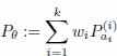
where ![]() are k-parametric models and A1,...,Ak are k sets in ℝdl,...,ℝdk with d1,...,dk ∈ ℕ* and 0 ≤ wi ≤ 1, ∑ wi = 1. Note that we consider a non-standard framework in which the weights are allowed to be equal to 0. Note Θ the parameter space
are k-parametric models and A1,...,Ak are k sets in ℝdl,...,ℝdk with d1,...,dk ∈ ℕ* and 0 ≤ wi ≤ 1, ∑ wi = 1. Note that we consider a non-standard framework in which the weights are allowed to be equal to 0. Note Θ the parameter space
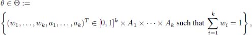
and assume that the model is identifiable. Let k0 ∈ {1, . . . , k – 1}.
We are willing to test if (k – k0) components in [8.28] have null coefficients. We assume that their labels are k0 + 1,..., k. Denote Θ0 the subset of Θ defined by
In this case, the test statistic 2nϕn (Θ0, θT):= 2n infθ∈Θ0 ϕn (θ, θT) converges to a ![]() distribution when H0 holds.
distribution when H0 holds.
While many divergences meet the former properties, we restrict ourselves to two generators in the following.
8.3.1.1. Chi-square divergence
The first divergence that we consider is the χ2 -divergence. The corresponding ϕ function ![]() is defined and convex on whole R; an example when P may contain signed finite measures and not be restricted to probability measures is considered in Broniatowski and Keziou (2006) in relation with a two-component mixture model defined in [8.24] and where θ is allowed to assume values in an open neighborhood Θ of 0, in order to provide a test for [8.26], with θ an interior point of Θ.
is defined and convex on whole R; an example when P may contain signed finite measures and not be restricted to probability measures is considered in Broniatowski and Keziou (2006) in relation with a two-component mixture model defined in [8.24] and where θ is allowed to assume values in an open neighborhood Θ of 0, in order to provide a test for [8.26], with θ an interior point of Θ.
8.3.1.2. Modified Kullback-Leibler divergence
The second divergence that we retain is generated by a function described below, namely
which has been derived within the recent general framework of Broniatowski and Stummer (2019). It is straightforward to see that φc is strictly convex and satisfies ![]() . For the special choice c = 0, [8.29] reduces to the omnipresent Kullback-Leibler divergence generator
. For the special choice c = 0, [8.29] reduces to the omnipresent Kullback-Leibler divergence generator
According to [8.29], in the case of c > 0 the domain ]1 – ec, ∞[ of ϕc also covers negative numbers (see Broniatowski and Stummer (2019) for insights on divergence-generators with general real-valued domain); thus, the same facts hold for the new generator as for the χ2 and this opens the gate to considerable comfort in testing mixture-type hypotheses against corresponding marginal-type alternatives, as we derive in the following. We denote KLc the corresponding divergence functional for which KLc(Q, P) is well defined, whenever P is a probability measure and Q is a signed measure.
It can be noted that, depending on the type of model considered, the validity of the test can be subject to constraints over the parameters of the densities. Indeed, the convergence of ![]() is not always guaranteed. This kind of consideration may guide the choice of the test statistic. For instance, in some cases, including scaling models, conditions that are required for the χ2 -divergence, do not apply to the KLc-divergence. For instance, consider a Gaussian mixture model with different variances
is not always guaranteed. This kind of consideration may guide the choice of the test statistic. For instance, in some cases, including scaling models, conditions that are required for the χ2 -divergence, do not apply to the KLc-divergence. For instance, consider a Gaussian mixture model with different variances
The convergence of I with the χ2 requires either ![]() . On the other hand, the convergence is always ensured with the KLc-divergence.
. On the other hand, the convergence is always ensured with the KLc-divergence.
The same observations can be made for the lognormal, exponential and Weibull densities. This fact enlightens the necessary interplay between the model and the statistical criterion, which should impose as little restriction as possible on the unknown part of the inference process. We refer to Broniatowski et al. (2019) for extensions to models with estimated parameters and numerical results.
8.4. References
Basu, A., Harris, I.R., Hjort, N.L., and Jones, M. (1998). Robust and efficient estimation by minimising a density power divergence. Biometrika, 85(3), 549–549.
Broniatowski, M., and Moutsouka, J. (2020). Smooth min-divergence inference in semi parametric models. [Online]. Available at: https://hal.archives-ouvertes.fr/hal-02586204.
Broniatowski, M., and Decurninge, A. (2016). Estimation for models defined by conditions on their L-moments. IEEE Transactions on Information Theory, 62(9), 5181–5181.
Broniatowski, M., and Keziou, A. (2006). Minimization of (ϕ-divergences on sets of signed measures. Studia Scientiarum Mathematicarum Hungarica, 43(4), 403–403.
Broniatowski, M., and Keziou, A. (2009). Parametric estimation and tests through divergences and the duality technique. Journal of Multivariate Analysis, 100(1), 16–16.
Broniatowski, M., and Keziou, A. (2012). Divergences and duality for estimation and test under moment condition models. Journal of Statistical Planning and Inference, 142(9), 2554–2554.
Broniatowski, M., Miranda, E., and Stummer, W. (2019). Testing the number and the nature of the components in a mixture distribution. Lecture Notes in Computer Science 11712. Geometric Science of Information - 4th International Conference. Springer, Cham.
Broniatowski, M., and Stummer, W. (2019). Some universal insights on divergences for statistics, machine learning and articial intelligence. In Nielsen, F. (ed.). Geometric Structures of Information. Springer, Cham.
Broniatowski, M., and Vajda, I. (2012). Several applications of divergence criteria in continuous families. Kybernetika, 48(4), 600 – 636.
Chen, H., Chen, J., and Kalbfleisch, J.D. (2001). A modified likelihood ratio test for homogeneity in finite mixture models. Journal of the Royal Statistical Society: Series B (Statistical Methodology), 63(1), 19–29.
Csiszár, I. (1964). Eine informationstheoretische Ungleichung und ihre Anwendung auf Beweis der Ergodizitaet von markoffschen Ketten. Magyer Tud. Akad. Mat. Kutato Int. Koezl., 8, 85 – 108.
Hampel, F.R., Ronchetti, E.M., Rousseeuw, P.J., Stahel, W.A. (1986). Robust statistics. The approach based on influence functions. John Wiley & Sons, Inc., New York.
Keziou, A., and Leoni-Aubin, S. (2008). On empirical likelihood for semiparametric two-sample density ratio models. Journal of Statistical Planning and Inference, 138(4), 915–928.
Liese, F., and Vajda, I. (1987). Convex Statistical Distances. BSB B.G. Teubner Verlagsgesellschaft, Leipzig.
Read, T.R.C., Cressie, N.A.C. (1988). Goodness-of-Fit Statistics for Discrete Multivariate Data. Springer-Verlag, New York.
Rényi, A. (1961). On measures of entropy and information. Proc. 4th Berkeley Sympos. Math. Statist. and Prob. University of California Press, Berkeley.
Titterington, D.M., Smith, A.F.M., and Makov, U.E. (1985). Statistical Analysis of Finite Mixture Distributions. John Wiley & Sons Ltd., Chichester.
Vajda, I. (1984). Minimum divergence principle in statistical estimation. Statistics and Decisions, 1, 239 – 261.
Vajda, I. (1986). Efficiency and robustness control via distorted maximum likelihood estimation. Kybernetika, 22(1), 47 – 67.
Chapter written by Michel BRONIATOWSKI.