
3
A Review of the Dividend Discount Model: From Deterministic to Stochastic Models
This chapter introduces a comprehensive overview of the dividend discount models, with a focus on the modeling of the dividend growth process. The analysis starts with the basic Gordon growth model and its extensions to more advanced models based on the Markov chain, leading the reader to the latest frontiers of the stock valuation.
3.1. Introduction
This chapter presents a review of the dividend discount models starting from the basic models (Williams 1938; Gordon and Shapiro 1956) to more recent and complex models (Ghezzi and Piccardi 2003; Barbu et al. 2017; D’Amico and De Blasis 2019) with a focus on the modeling of the dividend process rather than the discounting factor, that is assumed constant in most of the models. The chapter starts with an introduction to the basic valuation model with some general aspects to consider when performing the computation. Then, section 3.3 presents the Gordon growth model (Gordon 1962) with some of its extensions (Malkiel 1963; Fuller and Hsia 1984; Molodovsky et al. 1965; Brooks and Helms 1990; Barsky and De Long 1993) and reports some empirical evidences. Extended reviews of the Gordon stock valuation model and its extensions can be found in Kamstra (2003) and Damodaran (2012). In section 3.4, the focus is directed to more recent advancements in which the dividend process is modeled as a Markov chain (Hurley and Johnson 1994; Yao 1997; Hurley and Johnson 1998; Ghezzi and Piccardi 2003; Barbu et al. 2017; D’Amico and De Blasis 2019). The advantage of these models is the possibility to obtain a different valuation that depends on the state of the dividend series, allowing the model to be closer to reality. In addition, these models allow one to obtain a measure of the risk of the single stock or a portfolio of stocks. Finally, in section 3.5 some concluding remarks are made.
3.2. General model
Stock valuation is one of the basic aspects of financial markets. Discussions about the fair price of a stock, or its overpricing and underpricing, have always been of paramount importance to investors. Williams (1938) was the first to recognize that market prices and fundamental values are “separate and distinct things not to be confused”. In his work, he states that an asset’s intrinsic long-term value is the present value of all future cash flows, i.e. dividends and future selling price.
Let P (t) be the random variable giving the fundamental value of a stock at time t ∈ ℕ. Let D(t) be the dividend at time t ∈ ℕ also assumed to be a random variable, and denote by ke(t) the required rate of returm on the stock at time t. If we buy a stock at time t and plan to sell it at time t + 1, the price ![]() that we pay is the expected value of the stock price at time t + 1 plus the cash flows distributed by the company, all discounted at an appropriate measure of risk ke(t), given as
that we pay is the expected value of the stock price at time t + 1 plus the cash flows distributed by the company, all discounted at an appropriate measure of risk ke(t), given as
If we buy and hold the stock indefinitely, and assuming (see, for example, Samuelson 1973)
then the price we pay is the expected value of all future cash flows in the form of dividends,
If condition [3.2] is not assumed, then Blanchard and Watson (1982) proved that there could exist different solutions of the fundamental equation, i.e. there is a presence of bubbles in the stock market.
To solve equation [3.3], we have to identify two inputs, namely future dividends and the required measure of risk. When estimating future dividends, because of the impossibility of making predictions through to infinity, many models make assumptions about the dividend growth. The basic Gordon model (Gordon 1962) is based on a constant dividend growth rate, while multistage models are advanced by Brooks and Helms (1990) and Barsky and De Long (1993) to better describe the dividend growth series. Donaldson and Kamstra (1996) generalize the Gordon growth model to allow for arbitrary dividend growth and discount rates using a Monte Carlo simulation. On the contrary, other models apply specific stochastic processes to forecast dividends. Gutiérrez and Vázquez (2004) propose a model that allows a regime switching in the dividend process, and the Korn and Rogers (2005) model dividends as a deterministic transformation of a Lévy process. Hurley (2013) introduces dividends modeled as a Bernoulli process with a continuous set of values, while Eisdorfer and Giaccotto (2014) model the time series behavior of dividend growth rates with a first-order autoregressive process. In this chapter, we focus on how the various models make assumptions about the dividend process, with particular attention paid to the Markov chain based models.
The second input of the equation is the discount factor ke(t), or the cost of equity, that represents a measure of the asset’s riskiness. In most of the dividend discount models, it is assumed to be constant, ke. Traditionally, the estimation of ke has been performed using the capital asset pricing model (CAPM). This model originates from the idea of the mean-variance efficient portfolio of Markowitz (1952), and it is formalized by Sharpe (1964) and Lintner (1965) and extended by Black (1972). The rationale of the model is that risky investments Ri, e.g. stocks in financial markets, are expected to be more remunerating than the risk-free assets
where Rm is the return on the market portfolio, and Rf is the return on the risk-free asset. Black’s (1972) version substitutes the risk-free rate with a zero-beta portfolio uncorrelated with the market. The coefficient βim represents the correlation of the stock with the market and can be estimated as the slope coefficient of the ordinary least squares (OLS) regression
where Zit is the excess return of the stock on the risk-free asset, or equity premium, and Zmt is the market risk premium, ![]() . In practical applications, the market return and the risk-free rate are proxied by market indices, e.g. the S&P 500 Index, and government treasury bonds, respectively. The estimation is based on a period of time that generally extends to about 5 years of historical data (Campbell et al. 1997).
. In practical applications, the market return and the risk-free rate are proxied by market indices, e.g. the S&P 500 Index, and government treasury bonds, respectively. The estimation is based on a period of time that generally extends to about 5 years of historical data (Campbell et al. 1997).
Many authors provide empirical evidence on the CAPM application (see, for example, Jensen et al. 1972; Fama and MacBeth 1973; Blume and Friend 1973; Basu 1977; Fama and French 1992, 1993), while Roll (1977) criticizes it because the market portfolio is not observable and therefore the model is not testable. For a comprehensive description of the CAPM models and its variations with econometrics analysis, see, for example, Campbell et al. (1997) and Cochrane (2009).
In general, the dividend discount model is a very attractive model because it is intuitive and easy to implement. Nevertheless, it encounters much criticism because of the limits it poses. The main argument is the applicability of the model only to certain firms with stable, high-paying dividend policy. Moreover, the firms’ recent practice of performing share buybacks instead of paying dividends, for obvious tax reasons, reduces the dividend cash flow and the application of the dividend discount model results in an underestimation of the value of the firm. The same principle applies to other assets that are ignored in the model, e.g the value of brand names. However, share buybacks and values of other assets can be included in the dividends flow and treated as such with adequate adjustments (see, for example, Damodaran 2012).
3.3. Gordon growth model and extensions
In this section, we introduce the basic Gordon growth model that represents the cornerstone of the stock valuation. Then, we discuss some extensions, mainly based on the modeling of the dividend process, starting from the two-stage model up to the geometric or arbitrary dividend growth model.
3.3.1. Gordon model
Equation [3.3] can be rewritten in terms of dividend growth, defining
as the growth rate of dividends from time t to time t + 1, so that D(t+ 1) = D(t) (1 + g(t)) and D(t + 2) = D(t) (1 + g(t)) (1 + g(t + 1)) . Then, the price becomes
Assuming a constant dividend growth rate g(t + j) = g and a constant discounting factor ke (t + j) = ke, equation [3.8] becomes
and summing the geometric progression, we obtain the Gordon fundamental price estimate (Gordon 1962)
with the constraint g < ke to obtain a finite price.
The Gordon model is straightforward because it requires only estimates of the dividend growth rate and discount rate that are both easily obtained from a company’s historical data. Nevertheless, it has some limitations. The model can result in incorrect estimations of the price when the growth rate approaches the discount rate, as the price tends to grow up to infinity. Therefore, this model is more suitable for companies with a stable dividend policy with a growth that is less than the growth of the economy. Moreover, empirical applications of the Gordon model show that dividends tend to grow exponentially, meaning that a linear growth model is not suitable for the stock valuation (see, for example, Campbell and Shiller 1987; West 1988).
3.3.2. Two-stage model
The assumption that the dividends will experience constant growth forever is not realistic. To relax this assumption, Malkiel (1963) introduces a two-stage model, with the first period of n years of extraordinary growth followed by a stable growth forever. The value of a stock can be obtained as the sum of first years’ values, calculated from the general model plus a discounted value of the Gordon growth model at year n :
where PG (n) is the Gordon growth fundamental price estimate [3,10] at year n .
A further assumption of constant growth in the first phase, gh, and constant discount rate, ke,h, simplifies equation [3.11] to

This model is suitable for valuing companies that expect to have an initial growth period higher than normal, because of a specific investment or a patent right, that will result in higher profits. At the same time, it presents some limits. First, the growth rate is expected to drop drastically from high to normal level, and second, it is hard to define the length of the high growth period in practical terms.
3.3.3 H model
To avoid the sharp drop from high to stable growth rate, Fuller and Hsia (1984) propose a linear decline of the growth in their “H” model. The high growth phase with decline is assumed to last 2H periods up to the stable growth phase gn, with an initial growth rate ga. The model assumes that the discount rate ke is constant over time, as well as the dividend payout ratio, and it is given as follows:
A constant payout ratio assumption poses some limits to this model. Generally, a company is expected to have lower payout ratios in high growth phases and higher payout ratios in the stable growth phase, as shown in Figure 3.1.
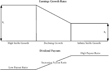
Figure 3.1. Expected growth in a three-stage dividend discount model (figure from Damodaran 2012, p. 341)
3.3.4. Three-stage model
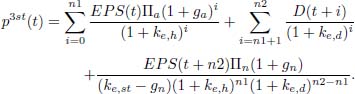
A three-stage model, initially formulated by Molodovsky et al. (1965) and derived from a combination of the H model and the two-stage model, with the inclusion of a variable payout policy and different discount factors for the various phases, overcomes the limits of previous models, but it requires a larger number of inputs. Let ke,h, ke,d and ke,st be the discount factors for high, declining, and stable phases, respectively. Let ga and gn be the growth rate at the beginning and the end of the period. Let EPS be the earnings per share, and Πa and Πn the payout ratios at the beginning and end of the period, respectively. The stock valuation for the three-stage model is
An empirical comparison of the Gordon model and its variations is in Sorensen and Williamson (1985). The authors analyze the intrinsic value of a random sample of 150 firms from the S&P 400 using data available in 1981 from four different valuation models, i.e. price/earning, constant growth, two-period and three-period models. They base the analysis on normalized earnings and a dividend payout ratio of approximately 45%. The discount factor is calculated using the CAPM model for the growth period, according to the beta of the stock and the high growth period is assumed to last 5 years for all the stock. Then, based on the assumption that all mature firms look alike, an equal risk measure of 8% among all the stocks is adopted for the stable phase.
For every model, the authors generate five portfolios of 30 stocks each, ordered from undervalued to overvalued securities, estimating returns for 2 years. Results show that the increased complexity of the model improves the annualized returns. As well as looking at the risk characteristics of the portfolios, the three-stage model outperforms the other model.
3.3.5. N-stage model
Brooks and Helms (1990) generalize the two-stage model from Malkiel (1963). They propose an N-stage model, with quarterly dividends and fractional periods. Within each stage, dividends growth is assumed as constant, and the discount rate is based on quarterly compounding ![]() . They test the model on the case of the Commonwealth Edison Company (CWE), an electricity supplier, estimating the required rate of return for three cases: (a) annual dividends, no fractional period; (b) quarterly dividends, no fractional periods; and (c) quarterly dividends, fractional periods. They show that ignoring quarterly compounding and fractional periods, the results present a downward bias.
. They test the model on the case of the Commonwealth Edison Company (CWE), an electricity supplier, estimating the required rate of return for three cases: (a) annual dividends, no fractional period; (b) quarterly dividends, no fractional periods; and (c) quarterly dividends, fractional periods. They show that ignoring quarterly compounding and fractional periods, the results present a downward bias.
3.3.6. Other extensions
Another extension of the Gordon growth models is given in Barsky and De Long (1993). The authors propose to model the permanent dividend growth as a geometric average of past dividend changes:
with g(t) following a random walk process and, thus, change in dividends following anIMA (1, 1)
Donaldson and Kamstra (1996) generalize the Gordon growth model, allowing for arbitrary dividend growth and discount rates. Their methodology involves a Monte Carlo simulation and numerical integration of the random joint process of dividend growth and discount rates
They forecast a range of possible evolution of the process y (t + 1) up to a certain point in the future, t + I, and calculate the average of several estimations of the present stock value
3.4. Markov chain stock models
According to equation [3.8] , the stock valuation is obtained through two inputs, namely the dividend growth and the discount factor. The idea of the Markov chain stock models is to describe the dividend growth rate as a sequence of independent, identically distributed discrete random variables, and model it as a Markov process. In all these models, the discount factor ke is kept constant.
3.4.1. Hurley and Johnson model
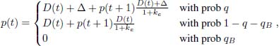
Hurley and Johnson (1994) model the dividend growth as a Markov dividend stream. They assume that in each period the dividend can increase with probability q, and can be constant with probability 1 – q, to resemble a step pattern in the long term. Moreover, they include the possibility for the firm to go bankrupt, with probability qB. They propose two variations of the model, an additive model and a geometric model, both giving an estimation of the value, along with a lower bound estimation for each of these values.
In the additive model, the dividend at time t + 1 increases by the amount Δ with probability q, and assuming a constant discount rate ke, the value of the firm is
and the closed-form solutions for the value and the lower bound are
and
Note that, when ![]() .
.
The geometric model assumes that the dividend increases with a growth rate g and with a probability q
The closed-form solutions for the value and the lower bound become
and
It is worth noting that the geometric model reduces to the Gordon model, setting the expected growth rate to qg – qB, or, if we exclude the possibility of bankruptcy, setting the expected growth rate to qg.
An empirical application to three stocks, provided in Hurley and Johnson (1994), shows that the geometric method performs well when the dividend series is erratic and does not always show increases. The model gives an estimation that is very close to the actual stock prices.
Hurley and Johnson (1998) formulate a generalized version of their model to include the possibility of a decrease in the dividends, so the dividend at time t is D(t) = D(t – 1) + Δi for the additive model, and D(t) = D(t – 1) (1 + gi) with probability qi for the geometric model. Both Δi and gi include the possibility of dividends reduction or suspensions. Under the condition ![]() , the closed-form solutions for both models are
, the closed-form solutions for both models are
and
When n = 1, the models reduce to Hurley and Johnson (1994) models.
3.4.2. Yao model
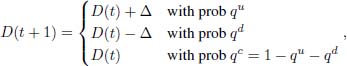
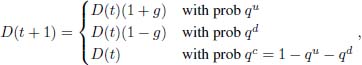
Yao (1997) advances the same proposal of a dividend reduction extending Hurley and Johnson (1994) models. The author introduces a trinomial dividend valuation model and extends the additive model, where the dividend at time t + 1 is
with closed solution for the stock value
Then, the geometric model, with
and closed solution
Lower bounds for both models are also given by the author. Moreover, a practical application on five firms, provided in Yao (1997), shows that the model produces better estimates than Hurley and Johnson (1994) models.
3.4.3. Markov stock model
Ghezzi and Piccardi (2003) start from the previous Markov models to formulate a more general Markov chain stock model. The authors begin with a description of the simple model for the dividend growth rate using a two-state discrete Markov chain, and a constant discount rate r = 1 + ke. Finally, they extend the model to an n-state Markov chain and define a vector of price–dividend ratios as the solution of a system of linear equations.
In previous models, Hurley and Johnson (1994, 1998) and Yao (1997) assume that the dividend growth rates are independent, identically distributed (i.i.d), discrete random variables, thus obtaining one closed-form solution irrespective of the state of the dividend. On the contrary, Ghezzi and Piccardi (2003) relax the i.i.d. assumption and obtain a different price–dividend solution for each state of the dividends. This variety allows the Markov chain stock model to be closer to reality.
The dividend series obeys the difference equation
where G(k + 1) is the dividend growth factor described by a Markov chain.
The dividend series relation [3.30] states that given the initial dividend value ![]() , we can compute the next random dividend D(1) = G(1) D(0) = G(1) d, D(2) = G(2) D(1) = G(2) G(1) d and so on. Generally,
, we can compute the next random dividend D(1) = G(1) D(0) = G(1) d, D(2) = G(2) D(1) = G(2) G(1) d and so on. Generally, ![]()
The combination of the dividend discount model equation [3.8] and [3.30] , with a constant discount factor r, i.e. one plus the required rate of return, yields
where d(k) and g(k) are the values at time k of the dividend process and of the growth–dividend process, respectively, and ψ1 (g(k)) is the price–dividend ratio.
The simple case is modeled with a two-state Markov chain taking values in the state space E = { g1, g2 }. Let P = (pij) i, j∈E be the one-step transition probability matrix of this Markov chain, and let
be the largest one step conditional expectation on the dividend growth rate.
If A1 holds true, then the series ![]() converges and satisfies the asymptotic condition in [3.2], and the pair (ψ1 (g1), ψ1 (g2)) is the unique and non-negative solution of the linear system
converges and satisfies the asymptotic condition in [3.2], and the pair (ψ1 (g1), ψ1 (g2)) is the unique and non-negative solution of the linear system

Assuming that for any given D(k), we obtain the same ![]() , irrespective of the initial states g1, g2, then p11 = q and p22 = 1 – q, therefore the solution to [3.33] becomes
, irrespective of the initial states g1, g2, then p11 = q and p22 = 1 – q, therefore the solution to [3.33] becomes
thus implying that the same price–dividend ratio is attached to each state, sharing the same results as Hurley and Johnson (1994, 1998) and Yao (1997) assume.
Results can be easily extended to the case of an s-state Markov chain with state space E = { g1, g2, …, gs } , where assumption A1 becomes
If ![]() the series [3.31] converges and the unique and non-negative solution to the linear system is
the series [3.31] converges and the unique and non-negative solution to the linear system is
This model has the advantage of assigning a different price–dividend ratio to each value of the states that does not depend on the time. Forecasts on the dividend growth rate are updated based on the previous value of the state, according to the Markov property, thus the price of the stock is updated according to the state of the dividend process. On the contrary, all previous models make fixed assumptions on forecasts and obtain a unique valuation.
Agosto and Moretto (2015) complement the model calculating a closed-form expression for the variance of random stock prices in a multinomial setting. The authors argue that for proper investment decisions, a measure of risk should be taken into consideration. Thus applying the standard mean-variance analysis, an investor can deal with financial decisions under uncertainty. In their model, they relate the variance of stock prices with the variance of the dividend rate of growth, obtaining a measure of the stock riskiness.
An extension of the Markov stock model is given in Barbu et al. (2017). The authors provide a formula for the computation of the second-order moment of the fundamental price process in the case of a two-state Markov chain,

To obtain the convergence of the series [3.37] and to satisfy the asymptotic condition in [3.2] and
the authors introduce a further assumption that avoids the presence of speculative bubbles,
where ![]() is the largest one-step second-order moment of the dividend growth rate.
is the largest one-step second-order moment of the dividend growth rate.
If assumptions A1 and A2 hold true, the pair (ψ2 (g1), ψ2 (g2)) is the unique and non-negative solution of the linear system
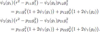
To extend the results to an s-state Markov chain with state space E = {g1, g2, …, gs} , assumptions A1 should be formulated as [3.35] and A2 as follows:
In this general case, systems [3.33] and [3.39] can be conveniently represented in the matrix form,
where:
- – Ψ1 = (ψ1 (g1), …, ψ1 (gn))⊤ and Ψ2 = (ψ2 (g1), …, ψ2 (gn))⊤
- – Ir : = rI, for any
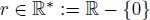 and, more generally,
- –
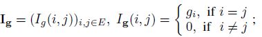
- – I is the identity matrix of dimension s × s
- – · denotes the row by column matrix product and ⋄ denotes the Hadamar delement by element product.
The matrix (Ir – P · Ig) is invertible, therefore system [3.41] has a unique solution,
Similarly, the matrix ![]() is invertible and the solution to system [3.42] is
is invertible and the solution to system [3.42] is
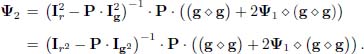
Relation [3.44] represents an explicit formula for the second-order price–dividend ratio that multiplied by d2(t) results in the second moment of the price process that is expressed as a function of the model parameters P and g.
Barbu et al. (2017) completed the Markov stock model framework developing non-parametric statistical techniques for the inferential analysis of the model where they propose estimators of price, risk and forecasted prices. For each estimator, they demonstrate that they are strongly consistent and that, after proper centralization and normalization, they converge in distribution to normal random variables. Finally, they give the interval estimators.
A further generalization of Ghezzi and Piccardi (2003) is available in D’Amico (2013). The author models the dividend growth rate as a semi-Markov chain. In this setting, prices become duration dependent. Therefore, they are influenced by the current state of the dividend growth process and by the elapsed time in the state. The same author proposes another extension of the model describing the dividend growth series via a continuous state space semi-Markov model (D’Amico 2017).
3.4.4. Multivariate Markov chain stock model
The previous analysis of the dividend discount model focused on the valuation of a single firm based on its dividend process. In this section, we analyze the problem of valuating multiple stocks when they constitute a financial portfolio. When dealing with more than one price series, it is important to consider the possible dependencies that characterize the pool of stocks. In a recent paper, Agosto et al. (2019) compute the covariance between two stocks that may be held in a portfolio. They consider a Markov chain with state space equal to the set of possible couples of the growth–dividend values for both stocks. However, this strategy cannot be easily implemented in real applications, especially when we introduce dependencies between more than two stocks as the number of parameters to estimate increase drastically.
D’Amico and De Blasis (2019) propose an extension of the Markov stock model to a multivariate setting, computing the first and the second-order price–dividend ratios. Moreover, the authors provide a formula for the computation of the variances and covariances between stocks in a portfolio. The model belongs to the class of mixture transition distribution models originated by Raftery (1985) in a high-order Markov chain setting and is further extended in Ching and Ng (2006) to a multivariate Markov chain setting. This approach makes it possible for one to overcome the limitations of Agosto et al. (2019) because it reduces the number of parameters to estimate.
With a portfolio of multiple stocks, α = 1, 2, …, γ, the dividend series expressed in [3.30] becomes
where {G(α) } k∈ℕ is the growth–dividend random process for stock α, and the multivariate Markov chain model follows the relationship,
where:
- –
 is a probability distribution vector with
 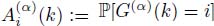 being the probability of growth–dividend of stock α to be at time k in state i;
 - –
 ;
; - – P(β, α) is the transition probability matrix of stock α given the state occupied one time step before by stock β, i.e
According to equation [3.46], the probability distribution function of the growth–dividend process at time k + 1 for the stock α depends on the state of the growth–dividend process of the same stock at time k, and, at the same time, on the set of states visited by each stock in the portfolio at time k.
To extend the model to a multivariate setting, the price process series [3.31] and [3.37] can be rewritten as
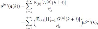

respectively. Equation [3.49] represents the fundamental formula of the price-product and reduces to the second-order moment of the price process when considering the same price series, α = β.
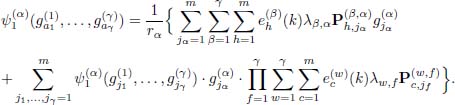
To guarantee the convergence of the series [3.48] and [3.49] in the multivariate setting. D’Amico and De Blasis (2019) extend the transversality conditions in [3.35] and [3.40],
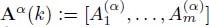
If assumptions in [3.50] holds true, then the first-order price–dividend ratio, ![]() can be computed as a linear system of mγ equations in mγ unknown that admits a unique solution,
can be computed as a linear system of mγ equations in mγ unknown that admits a unique solution,
Correspondingly, if assumptions in [3.50] and [3.51] hold true, then the secondorder price–dividend ratio, ![]() can be computed as a linear system of mγ equations in mγ unknown that admits a unique solution,
can be computed as a linear system of mγ equations in mγ unknown that admits a unique solution,
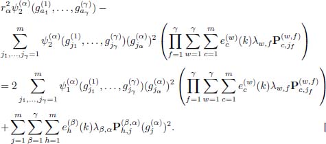
The solutions of the first- and second-order price–dividend ratio in [3.52] and [3.53] present a different price–dividend ratio attached to each combination of states of the growth process of each stock.
Finally, considering the possible correlation between the stocks and holding assumptions in [3.50] and [3.51], it is possible to compute the product price–dividend ratio, ![]() ,
,

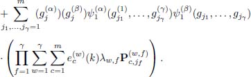
Knowing the product price–dividend ratio for any couple (α, β) of stocks, it is simple to compute the covariance function between the prices of two stocks:

The authors apply the model to a portfolio of three U.S. stock with a stable dividend policy with a long history and compare results with other valuation models. Finally, they show how to obtain the risk of the portfolio for different combinations of the stocks.
3.5. Conclusion
This chapter presented a review of the dividend discount model from its basic formulation to more recent and advanced stochastic models based on the Markov chain modeling of the dividend process. As the fundamental valuation of the firms represents an important function in the financial markets, especially for long-term investments, the Markov stock model clearly shows some advantages over the Gordon model and its extensions. In particular, the Markov stock model makes it possible for one to obtain a different valuation depending on the state of the growth–dividend process, or on a combination of the states of the various series in the multivariate case.
However, the Markov stock model presents some limitations that are shared with the other cited models. First, the valuation is based on the dividend process, therefore it is only applicable to companies that pay dividend and with a long history of payments. Second, the discounting factor, ke, is considered constant, thus it is not a realistic assumption when considering the very long timeframe.
Future extensions of the Markov stock model could consider the inclusion of some restrictions on the estimation of the transition probability matrix to reduce the number of parameters to estimate and permit the use of shorter dividend series.
Moreover, the cost of equity could be modeled as a stochastic process interdependent with the dividend process. Finally, the model could be extended to companies without a dividend policy, perhaps using the earnings or similar cash flows.
3.6. References
Agosto, A., and Moretto, E. (2015). Variance matters (in stochastic dividend discount models). Annals of Finance, 11(2), 283–295.
Agosto, A. Mainini, A., and Moretto, E. (2019). Stochastic dividend discount model: Covariance of random stock prices. Journal of Economics and Finance, 43(3), 552–568
Barbu, V.S., D’Amico, G., and De Blasis, R. (2017). Novel advancements in the Markov chain stock model: Analysis and inference. Annals of Finance, 13(2), 125–152
Barsky, R.B., and De Long, J.B. (1993). Why does the stock market fluctuate? The Quarterly Journal of Economics, 108(2), 291–311.
Basu, S. (1977). Investment performance of common stocks in relation to their price-earnings ratios: A test of the efficient market hypothesis. The Journal of Finance, 32(3), 66,–682
Black, F. (1972). Capital market equilibrium with restricted borrowing. The Journal of Business, 45(3), 444–455.
Blanchard, O.J., and Watson, M.W. (1982). Bubbles, rational expectations and financial markets. In Crises in the Economic and Financial Structure, Wachtel, P. (ed.). D.C. Heathand Company, Lexington.
Blume, M.E., and Friend, I. (1973). A new look at the capital asset pricing model. The Journal of Finance, 28(1), 19–34.
Brooks, R., and Helms, B. (1990). An n-stage, fractional period, quarterly dividend discount model. Financial Review, 25(4), 651–657.
Campbell, J.Y., and Shiller, R.J. (1987). Cointegration and tests of present value models. Journal of Political Economy, 95(5), 1062–1088.
Campbell, J.Y., Lo, A.W., and MacKinlay, A.C. (1997). The Econometrics of Financial Markets, vol. 2. Princeton University Press, NJ.
Ching, W.-K., and Ng, M.K. (2006). Markov Chains: Models, Algorithms and Applications. Springer, New York.
Cochrane, J.H. (2009). Asset Pricing, revised edition. Princeton University Press, NJ.
D’Amico, G. (2013). A semi-Markov approach to the stock valuation problem. Annals of Finance, 9(4), 589–610.
D’Amico, G. (2017). Stochastic dividend discount model: Risk and return. Markov Processes and Related Fields, 23(3), 349–376.
D’Amico, G., and De Blasis, R. (2019). A multivariate Markov chain stock model. Scandinavian Actuarial Journal, 2020(4), 272–291.
Damodaran, A. (2012). Investment Valuation: Tools and Techniques for Determining the Value of Any Asset. Wiley, New York.
Donaldson, R.G., and Kamstra, M. (1996). A new dividend forecasting procedure that rejects bubbles in asset prices: The case of 1929’s stock crash. The Review of Financial Studies, 9(2), 333–383.
Eisdorfer, A., and Giaccotto, C. (2014). Pricing assets with stochastic cash-flow growth. Quantitative Finance, 14(6), 1005–1017.
Fama, E.F. and French, K.R. (1992). The cross-section of expected stock returns. The Journal of Finance, 47(2), 427–465.
Fama, E.F., and French, K.R. (1993). Common risk factors in the returns on stocks and bonds. Journal of Financial Economics, 33(1), 3–56.
Fama, E.F., and MacBeth, J.D. (1973). Risk, return, and equilibrium: Empirical tests. Journal of Political Economy, 81(3), 607–636.
Fuller, R.J., and Hsia, C.-C. (1984). A simplified common stock valuation model. Financial Analysts Journal, 40(5), 49–56.
Ghezzi, L.L., and Piccardi, C. (2003). Stock valuation along a Markov chain. Applied Mathematics and Computation, 141(2–3), 385–393.
Gordon, M.J. (1962). The Investment, Financing, and Valuation of the Corporation. RD Irwin, Homewood, IL.
Gordon, M.J., and Shapiro, E. (1956). Capital equipment analysis: The required rate of profit. Management Science, 3(1), 102–110.
Gutiérrez, M.-J., and Vázquez, J. (2004). Switching equilibria: The present value model for stock prices revisited. Journal of Economic Dynamics and Control, 28(11), 2297–2325.
Hurley, W.J. (2013). Calculating first moments and confidence intervals for generalized stochastic dividend discount models. Journal of Mathematical Finance, 3(2), 275–279.
Hurley, W.J., and Johnson, L.D. (1994). A realistic dividend valuation model. Financial Analysts Journal, 50(4), 50–54.
Hurley, W.J., and Johnson, L.D. (1998). Generalized Markov dividend discount models. The Journal of Portfolio Management, 25(1), 27–31.
Jensen, M.C., Black, F., and Scholes, M.S. (1972). The capital asset pricing model: Some empirical tests. In Studies in the Theory of Capital Markets, Jensen, M.C. (ed.). Praeger, New York.
Kamstra, M. (2003). Pricing firms on the basis of fundamentals. Economic Review: Federal Reserve Bank of Atlanta, 88(1), 49–66.
Korn, R., and Rogers, L. (2005). Stocks paying discrete dividends: Modeling and option pricing. Journal of Derivatives, 13(2), 44.
Lintner, J. (1965). Security prices, risk, and maximal gains from diversification. The Journal of Finance, 20(4), 587–615.
Malkiel, B.G. (1963). Equity yields, growth, and the structure of share prices. The American Economic Review, 53(5), 1004–1031.
Markowitz, H. (1952). Portfolio selection. The Journal of Finance, 7(1), 77–91.
Molodovsky, N., May, C., and Chottiner, S. (1965). Common stock valuation: Principles, tables and application. Financial Analysts Journal, 21(2), 104–123.
Raftery, A.E. (1985). A model for high-order Markov chains. Journal of the Royal Statistical Society: Series B (Methodological), 47(3), 528–539.
Roll, R. (1977). A critique of the asset pricing theory’s tests Part I: On past and potential testability of the theory. Journal of Financial Economics, 4(2), 129–176.
Samuelson, P.A. (1973). Proof that properly discounted present values of assets vibrate randomly. The Bell Journal of Economics and Management Science, 4(2), 369–374.
Sharpe, W.F. (1964). Capital asset prices: A theory of market equilibrium under conditions of risk. The Journal of Finance, 19(3), 425–442.
Sorensen, E.H., and Williamson, D.A. (1985). Some evidence on the value of dividend discount models. Financial Analysts Journal, 41(6), 60–69.
West, K.D. (1988). Dividend innovations and stock price volatility. Econometrica, 56(1), 37–61.
Williams, J.B. (1938). The Theory of Investment Value. Harvard University Press, Cambridge.
Yao, Y.F. (1997). A trinomial dividend valuation model. The Journal of Portfolio Management, 23(4), 99–103.
Chapter written by Guglielmo D’AMICO and Riccardo DE BLASIS.