
We kick the book off by looking at classical algorithms for exact search, that is, finding positions in a string where a pattern string matches precisely. This problem is so fundamental that it received much attention in the very early days of computing, and by now, there are tens if not hundreds of approaches. In this chapter, we see a few classics.
Naïve algorithm

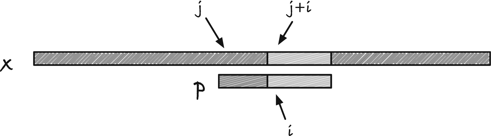
Exact search with the naïve approach
We terminate the comparison of x[i + j] and p[i] when we see a mismatch, so in the best case, where the first character in p never matches a character in x, the algorithm runs in time O(n) where n is the length of x. In the worst case, we match all the way to the end of p at each position, and in that case, the running time is O(nm) where m is the length of p.
makes sure that it is possible to match the pattern at all and that the pattern isn’t empty. This is something we could also test when we initialize the iterator. However, we do not have a way of reporting that we do not have a possible match there, so we put the test in the “next” function.
Border array and border search
It is possible to get O(n + m) running times for both best and worst case, and several algorithms exist for this. We will see several in the following sections. The first one is based on the so-called borders of strings.
Borders and border arrays

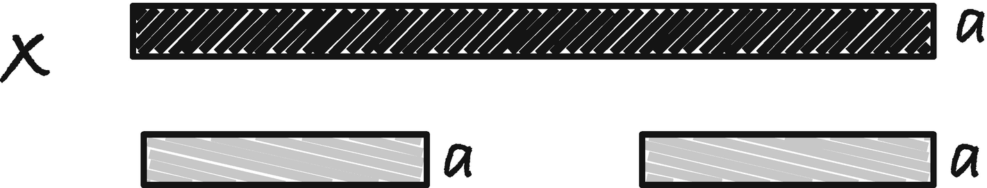
A string with three borders
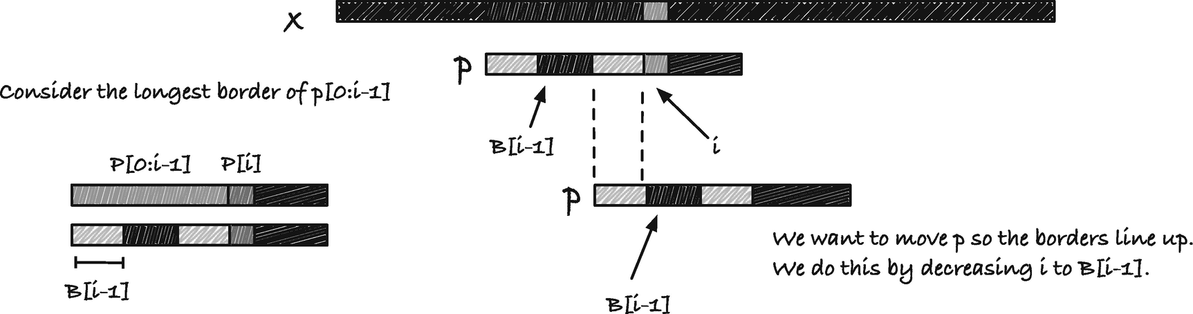
We can make the following observation about borders and border arrays: The longest border of x[0, i] is either the empty string or an extension of a border of x[0, i − 1]. If the letter at x[i] is a, the border of x[0, i] is some string y followed by a. The y string must be both at the beginning and end of x[0, i − 1] (see Figure 2-3), so it is a border of x[0, i − 1]. The longest border for x[0, i] is the longest border of x[0, i − 1] that is followed by a (which may be the empty border if the string x begins with a) or the empty border if there is no border we can extend with a.
Another observation is that if you have two borders to a string, then the shorter of the two is a border of the longer; see Figure 2-4.
Extending a border
A shorter border is always a border of a longer border

Searching for the longest border we can extend with letter a
The running time is m for a string x of length m. It is straightforward to see that the outer loop only runs m iterations but perhaps less easy to see that the inner loop is bounded by m iterations in total. But observe that in the outer loop, we at most increment b by one per iteration. We can assign b + 1 to ba[i] in the last statement in the inner loop and then get that value in the first line of the next iteration, but at no other point do we increment a value. In the inner loop, we always decrease b—when we get the border of b − 1, we always get a smaller value than b. We don’t allow b to go below zero in the inner loop, so the total number of iterations of that loop is bounded by how much the outer loop increase b. That is at most one per iteration, so we can decrement b by at most m, and therefore the total number of iterations of the inner loop is bounded by O(m).
Exact search using borders
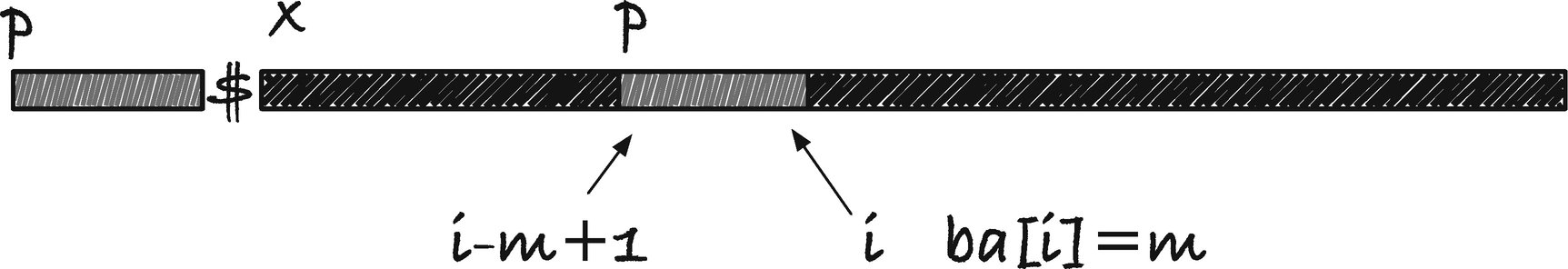
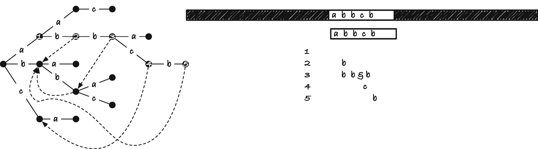
The reason we built the border array was to do an exact search, so how does the array help us? Imagine we build a string consisting of the pattern we search for, p, followed by the string we search in, x, separated by a sentinel, $ character not found elsewhere in the two strings, y = p$x. The sentinel ensures that all borders are less than the length of p, m, and anywhere we have a border of length m, we must have an occurrence of p (see Figure 2-6). In the figure, the indices are into the p$x string and not into x, but you can remap this by subtracting m + 1. The start index of the match is i − m + 1 rather than the more natural i − m because index i is at the end of the match and not one past it.
Searching using a border array
When we report an occurrence, we naturally set the position we matched in the report structure, and we remember the border and index positions.
Knuth-Morris-Pratt
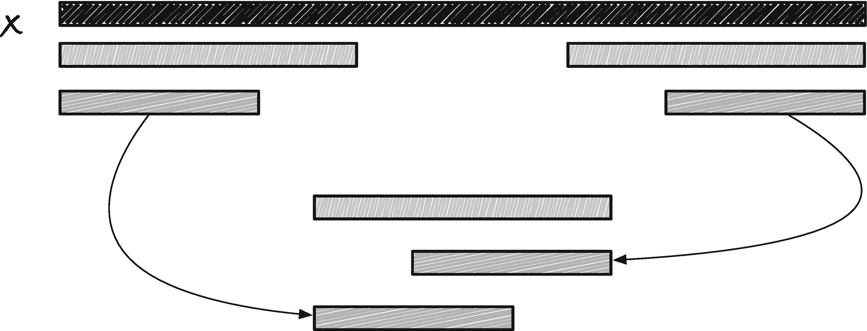
The Knuth-Morris-Pratt (KMP) algorithm also uses borders to achieve a best- and worst-case running time of O(n + m), but it uses the borders in a slightly different way. Before we get to the algorithm, however, I want to convince you that we can, conceptually, move the pattern p through x in two different ways; see Figure 2-7. We can let j be an index into x and imagine p starting there. When we test if p matches there, we use a pointer into p, i, and test x[ j + i] against p[i] for increasing i. To move p to another position in x, we change j, for example, to slide p one position to the right we increment j by one. Alternatively, we can imagine p aligned at position j − i for some index j in x and an index i into p. If we change i, we move j − i so we move p. If, for example, we want to move p one step to the right, we can decrement i by one. To understand how the KMP algorithm works, it is useful to think about moving p in the second way. We will increment the j and i indices when matching characters, but when we get a mismatch, we move p by decrementing i.

Two ways to conceptually look at matching

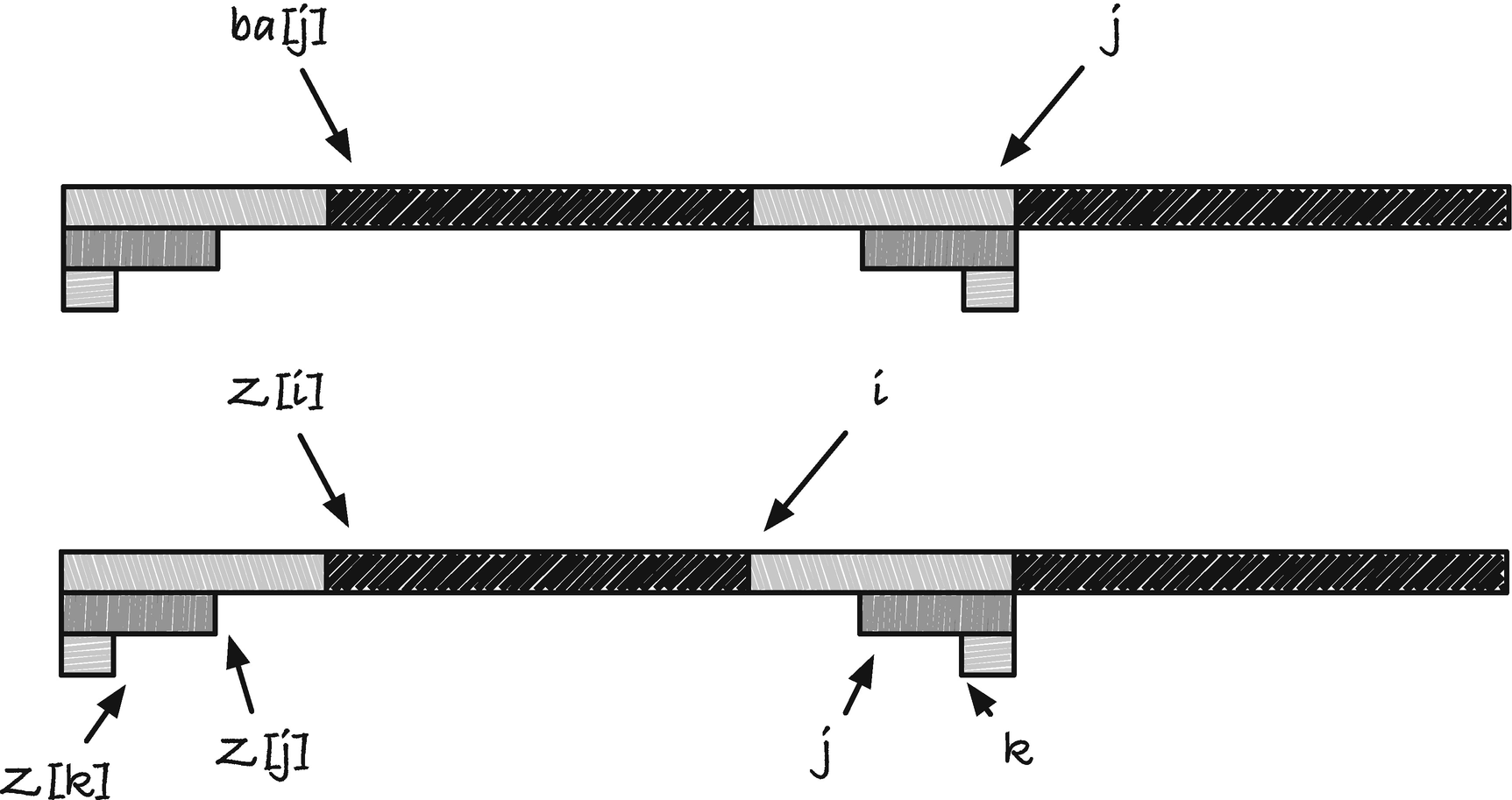
Borders and the observation underlying the KMP algorithm
Calculations for how much we should jump at a mismatch
The reason we have a Boolean for when we have a match is that we need to update the indices whether we have a match or not. I chose this solution to avoid duplicated code, but you could also have the update code twice instead.
Matching from right to left
Boyer-Moore-Horspool
With the Boyer-Moore-Horspool (BMH) algorithm , we are back to a worst-case running time of O(nm), but now with a best-case running time of O(n/m + m), that is, a potential sublinear running time. The trick to going faster than linear is to match the pattern from right to left (see Figure 2-10), which lets us use information about the match after the current position of p. If we have a mismatch before we reach the first character in p, that is, before we reach index j in x, we might be able to skip past the remaining prefix of x[ j, j+m] without looking at it.
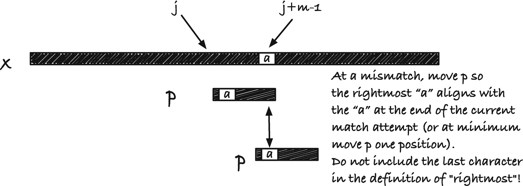
Observation that lets us jump ahead after a mismatch
It should be obvious that the preprocessing is done in O(m).
In our BMH iterator, we need to store the current position of p in x, j, and we need to store the jump table.
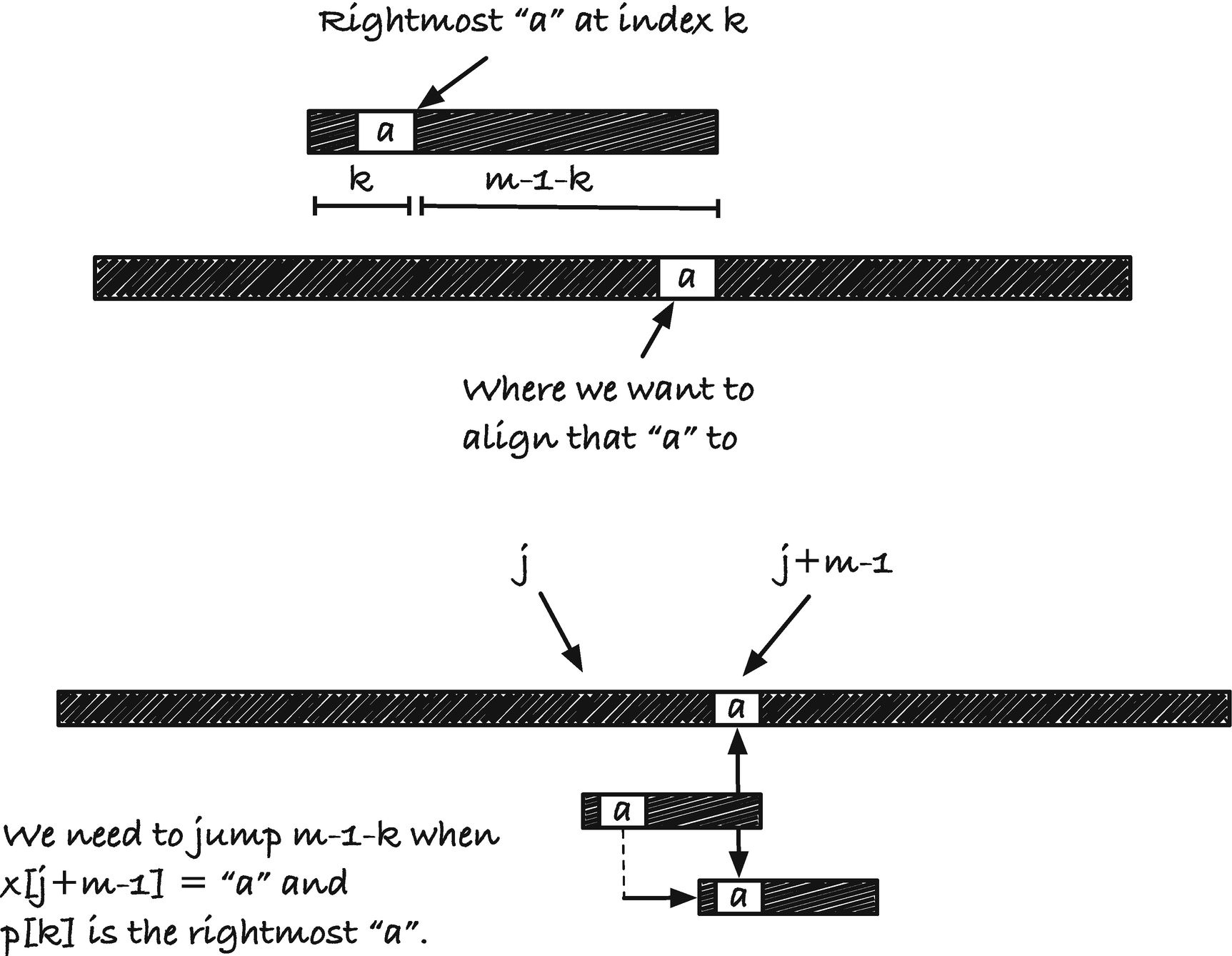
The length to jump at a mismatch
To see that the worst-case running time is O(nm), consider a string and a pattern that has only one character, x = aaa · · · a, p = aaa · · · a. With these two strings, we never have a mismatch, the rightmost occurrence of a (excluding the last character in p as we do) is m − 2, so we jump m − 1 − k with k = m – 2, which moves us one position to the right. So at each position in x, we match m characters, which gives us a running time of O(nm). For the best-case running time, consider x = aaa · · · a again but now the pattern p = bbb · · · b. We will always get a mismatch at the first character we see, and then we need to move to the rightmost occurrence of a in p. There isn’t any a in p, so we move p all the way past position j + m − 1. This means that we only look at every mth character and we, therefore, get a running time of O(n/m +m), where the m is for the preprocessing. These two examples are, of course, extreme, but with random strings over a large alphabet, or with natural languages, the rightmost occurrence can be far to the left or even not in the string, and we achieve running times close to the best case bound.

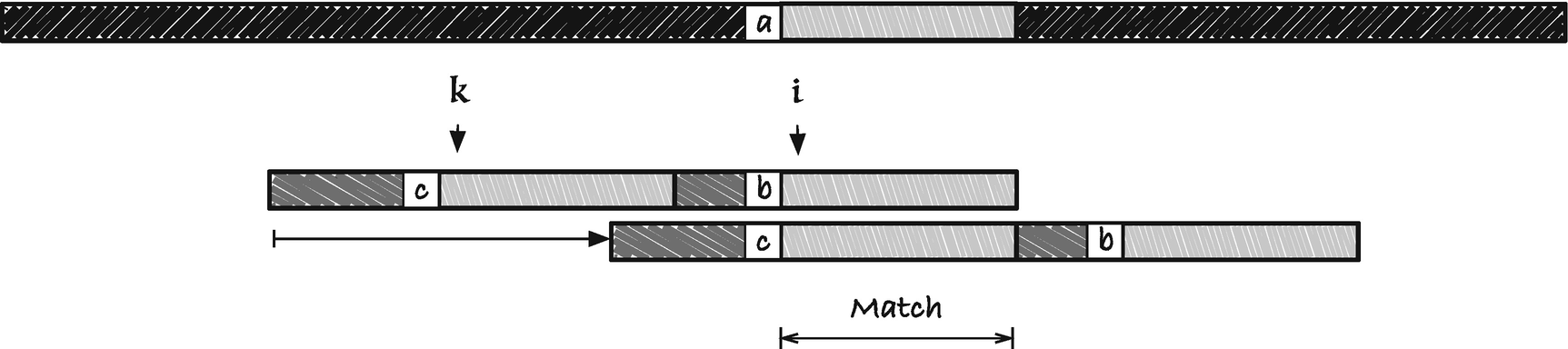
Second jump rule for BMH
The various variables in the macro are not arguments but hardwired to be used inside the algorithm. This makes it easier to see what the intent of the macro is inside the function and is an approach I will often take in this book.
Extended rightmost table
You might object, now, that the search in the lists is not constant time, so the running time now potentially exceeds O(nm + m) in the worst case. To see that this isn’t so, consider how many links we have to search through. The only indices that are larger than i are those m − i we scanned past before a jump. The first link after that will have an index smaller than i and we return that immediately. This means that the search in the list is not more expensive than the scan we just did in the string, so the running time is at most twice as many operations as without the lists, so worst case O(nm + m) and best case O(n/m + m).
Boyer-Moore
Jump rule one
As you can see from the figure, we shift p to the right to match up a substring with a suffix. This suffix is a border of the string p[k, n]. The border array we used in the first, nontrivial, algorithm gives us, for each i the longest border of p[0, i + 1], and this border is a prefix of the string. We need a suffix, so we use a corresponding border array computed from the right. We call it the reversed border array . Since we want the preceding characters to mismatch, we modify the reversed border array the same way as for the usual border array, but from the right to take care of preceding characters. Let us call this the restricted reversed border array , just to have something to call it. We shall use a variant of this array to compute the first jump table. There will not always be an occurrence of p[i, m] to the left of the suffix p[i, m], in which case this jump rule cannot be used. When this is the case, we set the jump rule to zero. Since the character rules in the BMH algorithm ensure that we always step at least one position to the right, and we will take the largest step possible between the two rules in this section and the two rules in the previous section, we will always move forward.

Jump rule two
Jump rule one
Here, I have split the computation into multiple functions to make it clear what each step is. I prefer the reverse-compute-reverse strategy in most cases, because though it is slightly less efficient it greatly minimizes the work necessary to implement both directions and reduces the risk of errors since there are fewer lines of code.

Jump table based on reverse borders
We go from left to right and let each suffix that also occurs internally in p and know about the position where it occurs. We do not add the matching part of the suffix to the jump table since we want to jump when we have a mismatch, so we get the index at the position left of the matching suffix. At the matching suffix, we insert in the jump table the length we should jump, n − xrba[i] − i. Because we do this from left to right, if there is more than one occurrence, we will get the rightmost one.

Example of backward border array and restricted backward border arrays
Border array jump table

Point to border endpoints rather than start points

Uniqueness of endpoints
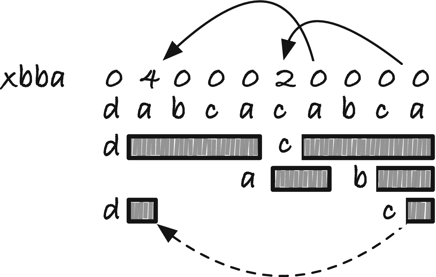
The Z array
In the Z array, p[0, Z[i]] = p[i, i + Z[i]] is the longest border of p[0, i + Z[i]]. We cannot extend it to the longest border of p[0, i +Z[i]+1] because p[Z[i]+1] ≠ p[i +Z[i]+1] since otherwise the longest string starting in i that matches a prefix of p would be at least one longer. With the Z array, we get the “restricted border” effect for free in this sense. For the reversed Z array, the same is true but for the letter that precedes the border strings.
Computing the Z array
The match() function works on pointers to strings and compares them as long as they haven’t reached the null sentinel and as long as they agree on the current character. If our string consists of only one character, x = an, then match() will run through the entire string x[i, n] which averaged over all the indices as O(n), giving us a total running time of O(n2). We can do better!
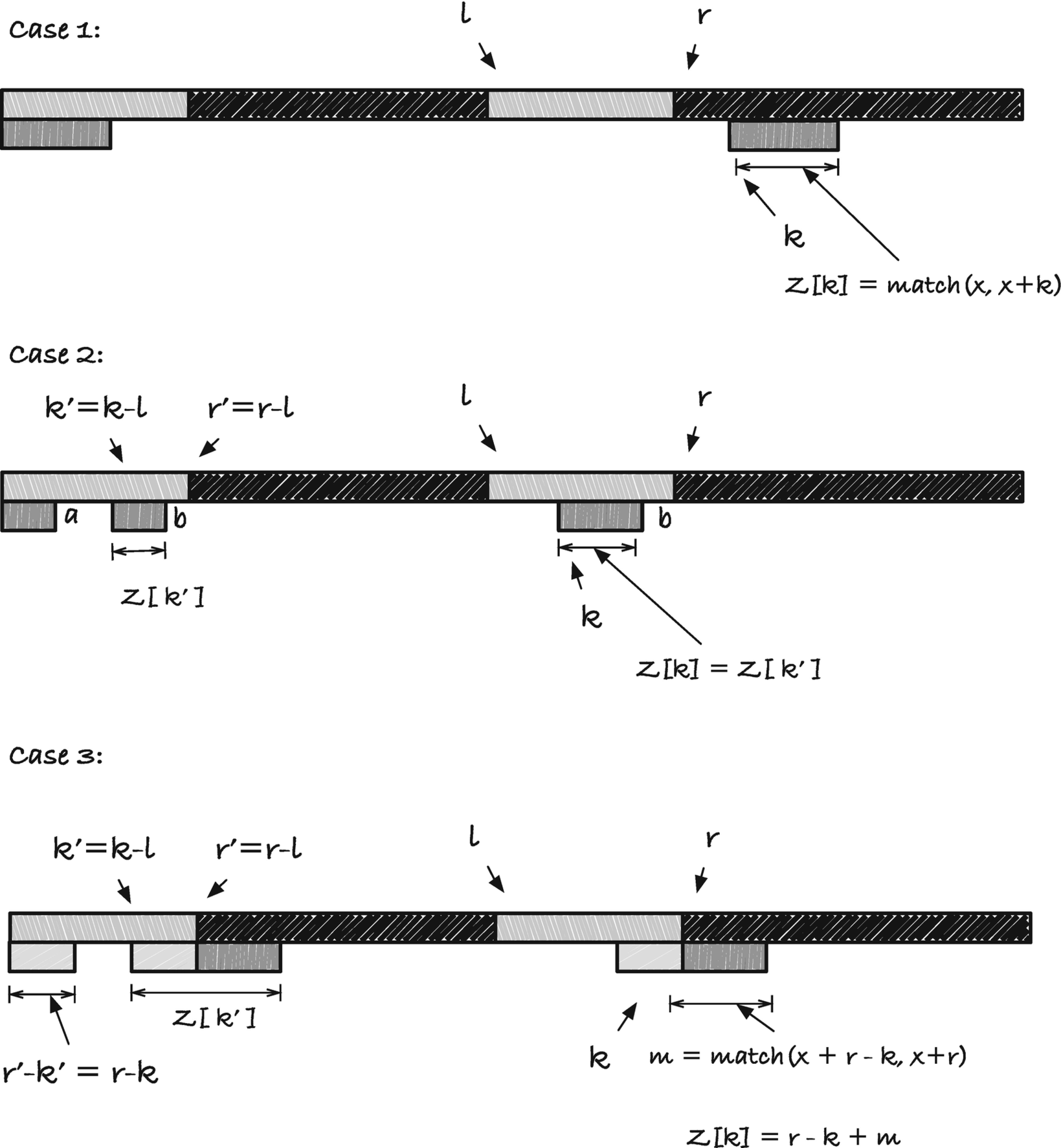
In a linear-time construction algorithm, we iteratively consider indices k = 0, 1, ..., n − 1 and compute Z[k] using the previously computed values. We let l and r denote the leftmost index and one past the right index, respectively, of the rightmost string we have seen so far. As invariants in the algorithm, we have for all k' < k that Z[k'] is computed and available and that l and r index the rightmost string x[l, l + Z[l]] seen so far.
There are three cases to consider; see Figure 2-22. The first is when the index we are computing is to the right of r. We can get in this situation if we have seen a rightmost string pointed to by l and r, but the following ks gave us empty borders. To get Z[k] we must compare x with x + k to get the matching length. If this length is zero, we set Z[k] to zero and move to k + 1. If the match result is greater than zero, we set Z[k] to the value and move l to k and r to k + Z[k]; the rightmost string we have seen is now then one starting in k, and the updated indices will point at it.
The three cases for the Z array construction algorithm
Case three is when the string starting at index k' continues past index r'. In this case, we know that a prefix of the string matches a suffix of the string x[l, r], but we do not know how much further the prefix will match the string starting at index k. To find out where, we must do a character-by-character match. We do not need to start this search at index 1 and k, however. We know that the first r − k characters match, so we can start our match at indices r − k and r; see case three in Figure 2-22. When we have found the right string, we update the left pointer to point at the start of it, l = k, and we set the right pointer to the end of the string r = k + Z[k].
To see that the running time is linear, first ignore the calls to match() . If we do, we can see that there are a constant number of operations in each case, so without matching, we clearly have a linear running time. To handle match(), we do not consider how much we match in each iteration—something that depends on the string and that we do not have much control over. Instead, we consider the sum of all matches in a run of the algorithm. We never call match() in the second case, so we need only to consider cases one and three. Here, the key observation is that we only search to the right of r and never twice with the same starting position.
In case one, we either have a mismatch on the first character, or we get a new string back. In the first case, we leave l and r alone and immediately move to the next k, which we will use as the starting point for the next match. As long as we are not getting a string back from our matching, we use constant time for match() calls for each k, and we never call match() on the same index twice. If we get a string, we move the right pointer, r, to the end of this string. We will never see the indices to the left of r again because both case one and three never search to the left of r. In the search in case three and a nontrivial result in case one, we always move r past all indices we have started a search in earlier.
Z-based jump table
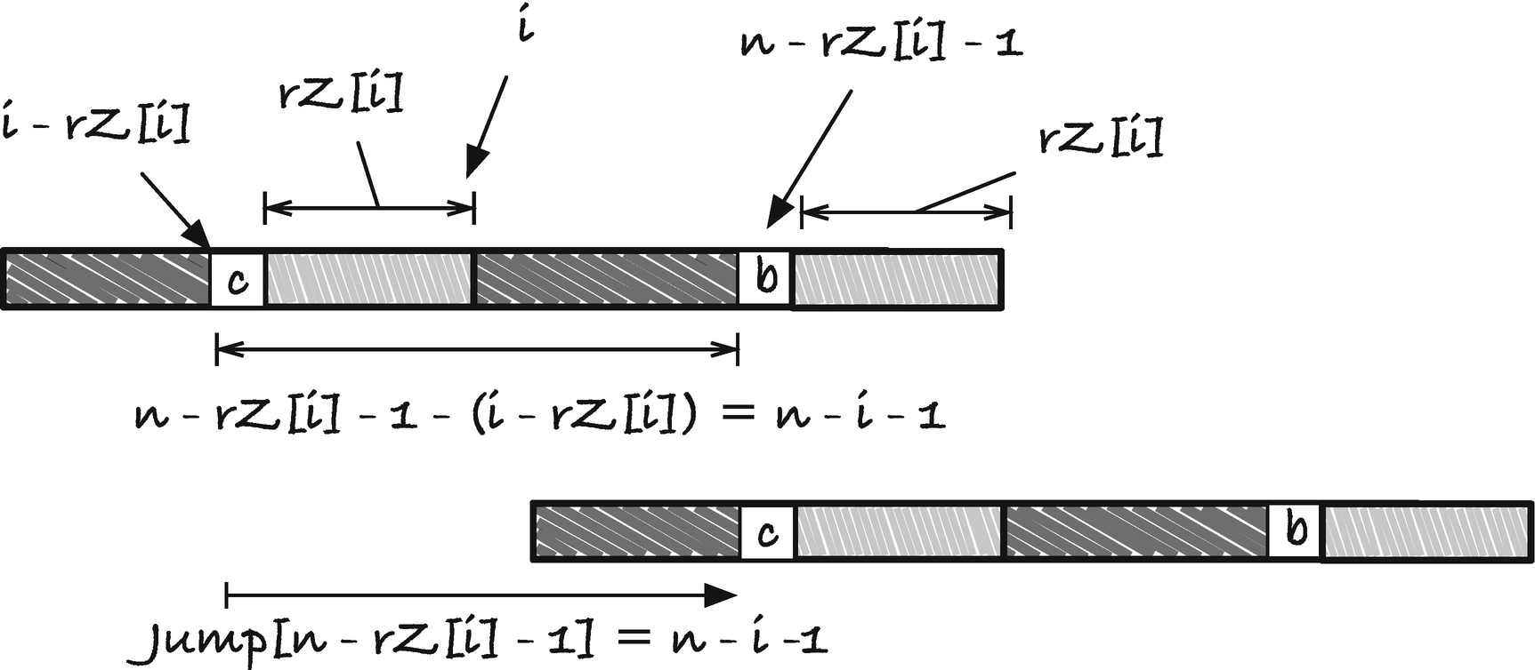
The jump rule needs to slide p to the rightmost position where we potentially have a match. If i is where the rightmost occurrence sits, then index i − rZ[i] is the character just before the start of the occurrence. If there is no occurrence, we set the jump distance to zero, which leaves it up to one of the other jump rules. The prefix it matches starts at position n − rZ[i], and it is when we have a mismatch p[i − rZ[i]] ≠ p[n − rZ[i] − 1] we should move p. Therefore, we want to store the jump distance for index n−rZ[i]−1 in our jump table. The distance we need to jump is the one that places i −rZ[i] at position n −rZ[i]−1, so n −rZ[i]−q −(i −rZ[i]) = n − i − 1. See Figure 2-23 for an illustration of the jump rule and Figure 2-24 for a concrete example.
First jump rule for Boyer-Moore
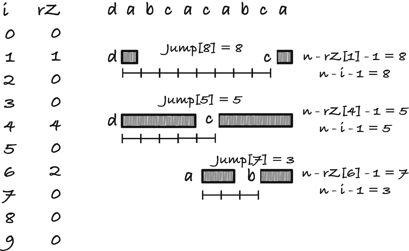
Boyer-Moore jump table one example
We do this in the iterator initialization . We will see the full initialization later when we have seen the second jump table as well.
We do not test for whether the reverse Z value is zero. In this case, we want the jump to be zero (so we will use one of the other jump rules), but whenever Z is zero, the loop will update the last index, n − rZ[i] − 1 = n − 1. In the final iteration, we will write n − i − 1 = n − (n − 1) − 1 = 0 there, exactly as desired.
Second jump table

Jump ranges for jump rule two
We include the border of size zero in this preprocessing. It will guarantee us that if we have matched a string that cannot be matched anywhere else in the pattern, then we skip the entire string past the current attempted match.
Combining the jump rules
With all these jump tables, the Boyer-Moore algorithm is more complicated than the previous algorithms. Still, if we put the border and Z array functionality in separate functions, then the BM iterator is not overly complex to initialize and use.
Aho-Corasick
The Aho-Corasick algorithm differs from the previous algorithms in that it does not only search for a single pattern but search simultaneously for a set of patterns. The algorithm uses a data structure, a trie (short for retrieval), that can store a set of strings and provide efficient lookups to determine if a given string is in the set.
Tries
A trie, also known as a prefix tree , is a tree where each edge holds a letter and where no child has more than one out edge with the same letter. Going from the root and down, you can read off all prefixes of one or more of the strings in the set, and when you have seen a full string from the set, you reach a node that is tagged with the string label from the set; see Figure 2-26.
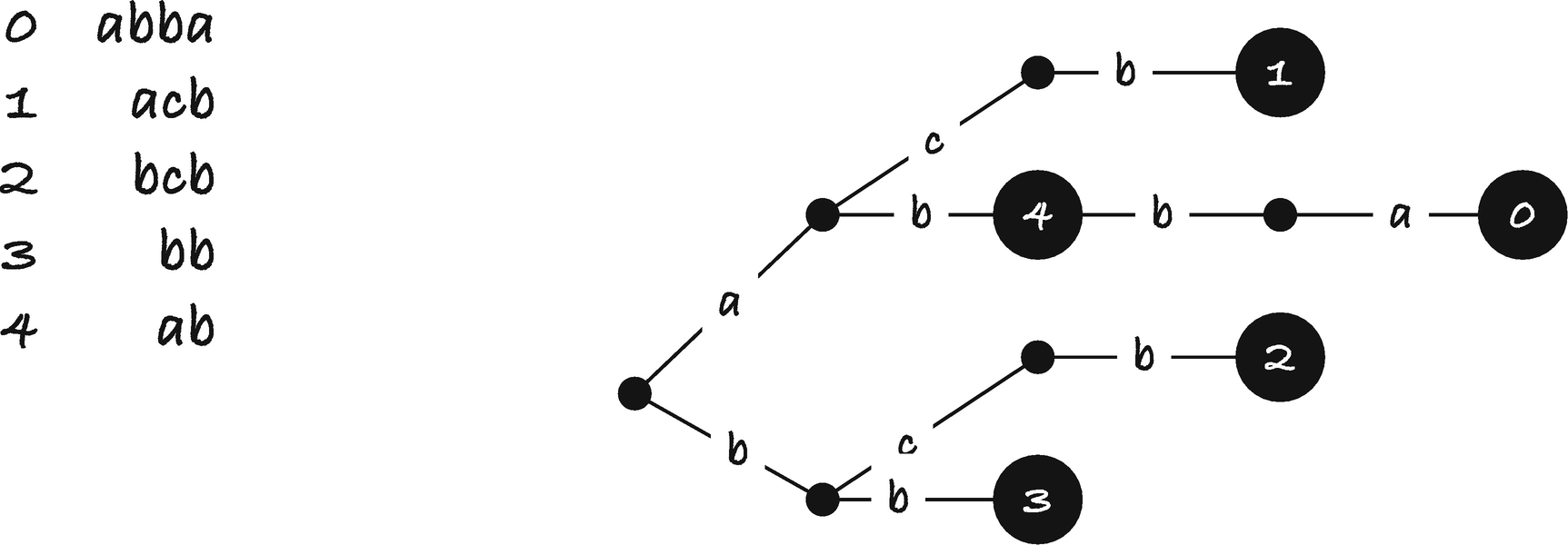
The trie data structure

A trie with sentinel strings
The parent pointer isn’t needed in many algorithms, but we need it in the Aho-Corasick algorithm, so I have included it here. As an example, Figure 2-28 is the representation of the trie in Figure 2-26. Notice that the child pointer points to tries. This is because all sub-tries are also tries themselves.

Representing a trie in C
I have written two functions for initializing tries, one that assumes that you have already allocated a root struct trie structure and one that does it for you. When you want a new trie, you create its root using one of these functions. The root has no siblings, but it will have children once we add strings to it.
To construct a trie, we insert the input set string by string. When we add the string pi, we search down the trie, T, and either find an existing node at the end of pi, or we find that we cannot continue searching beyond some point k, that is, pi[0, k] matches, but there is no edge with character label pi[k]. In the first case, we set the node’s string_label to i, and in the second case, we must insert the string pi[k, m] in the node we reached before we couldn’t go any longer. So the straightforward approach is to find out where the string sits or where it branches off the trie and insert it there.
It starts from the end of the string and iteratively constructs a node for each letter, and sets that node’s child to the previous node we created. It sets the string label in the root and then updates the string_label variable , so the remaining nodes will be set to -1 indicating that they are not representing a string.
I split them into two functions because you sometimes want to get the node where a string is so you can do something with it. You cannot use get_trie_node() directly as a test. It returns a node or null, so you can test if there is a node on the path given by the string, but to test if it is in the trie’s set of strings, you must also check the string label. The string_in_trie() function does that.
First, assume that we can always find the out edge with a given symbol in constant time. We use linked lists for this, so on the surface this doesn’t seem to be the case, but we will always assume that the alphabet is of constant size, making a list search a constant time operation. When we insert pattern pi of length mi, we will in worst case search down mi steps down the trie, so if m = ∑imi, then the running time for constructing a trie is O(m).
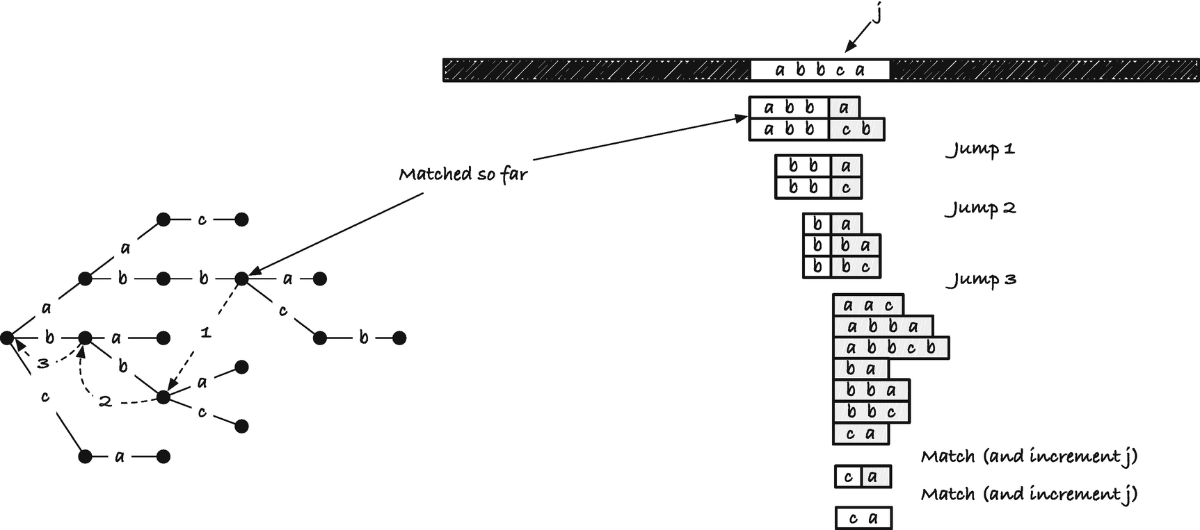
Matching and mismatching in Aho-Corasick
When we match along x, we move down the trie, matching character by character. All strings below the current position in the trie can potentially match x. If we have a mismatch, we need to move the trie to the right to the next position where we can potentially match. Consider any string you can read by concatenating the edge labels from the root and down the trie. That is, consider any string in the trie but not necessarily one labelled with the strings the trie contains. For such a string, p, let f (p) denote the longest proper suffix of p that you can also find in the trie. We call this mapping from p to f (p) the failure link of p because we will use it when we fail at matching deeper into the trie than p.
p | f (p) |
|---|---|
aac | ? |
abbcb | b |
ba | a |
bba | ba |
bbc | c |
ca | a |
abb | bb |
bb | b |
B | ? |
abba | bba |
Recall that ? denotes the empty string.
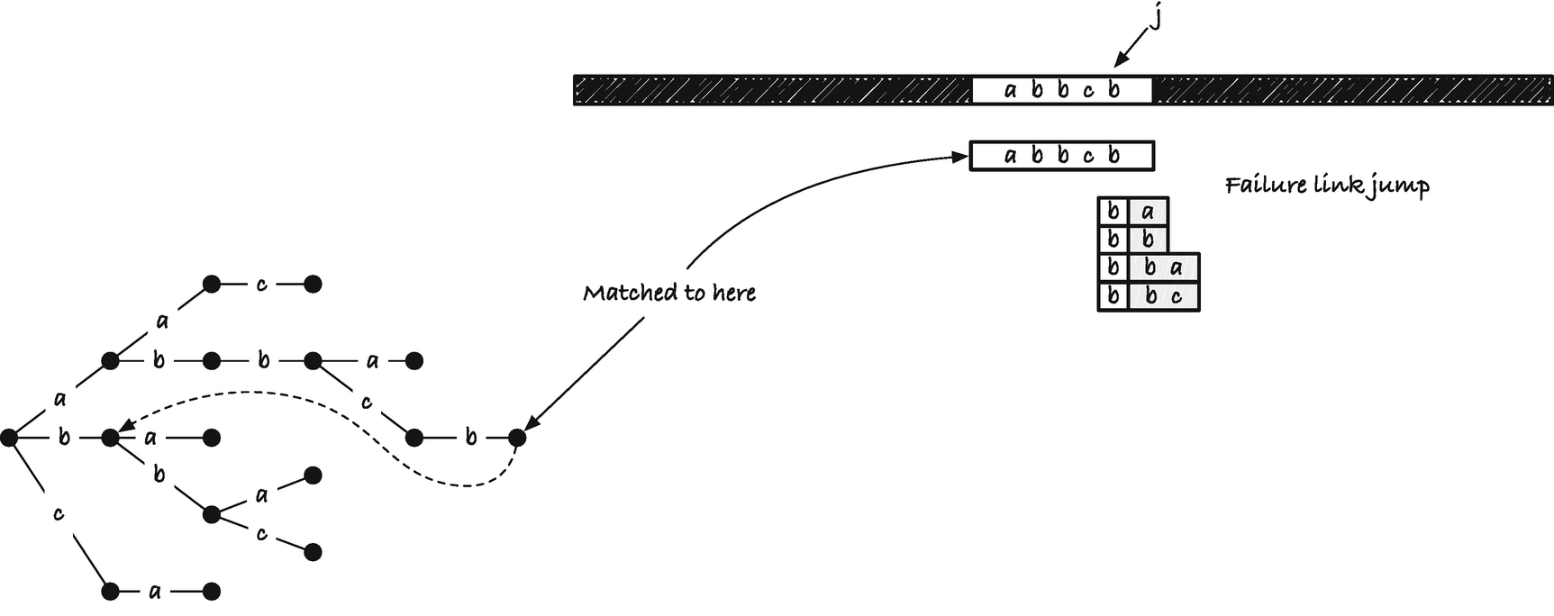
In the Aho-Corasick algorithm, we will represent failure links as pointers from each node to its failure link node. For nodes where the failure link is empty, we will set the pointer to point at the root of the trie. We will compute the failure nodes in a preprocessing step. Whenever we have a mismatch in the algorithm, we will move from the current node to its failure link—conceptually moving the trie further along x.
Problem with missing matches when one string is a substring of another
Output lists and matches
What we want to do is output all strings that match at a position, and all such strings can be found by traversing the failure links of the nodes; see Figure 2-31. All strings that match from a node we have reached in the trie must be suffixes of the current string in the trie, and we can get all of them by running through the failure link.
When we match the first character in abbcb, we do not match any additional string in the trie, but when we match ab, we also have a match of b that ends in this position. We can get that from following the failure link. When we match abb, we should also report a match of bb and b, and we can get those by following the failure link twice, first for bb and then for b. When we match c, we should report c, and again we can see this using the failure link. Finally, when we match the last b in the string, we should report b as well as the full string. Unlike in this example, we do not want to output all nodes we can find from the failure links but only those with a nonnegative string label. So we skip those that do not by pointing to the next that does. The list we get from doing this is what we call the output list .
For each string v in the tree, you can go through the failure links v, f (v), f2(v), ..., fn (v) from the node up to the root. Each link, by definition, is closer to the root than the previous, so we will eventually get there. From the nodes you see on this path, extract those with a nonnegative string label. That is the output list.
To see that we output all matches that end at index j when we run through the output list, observe that when we move through the failure links, we get all the strings that match a suffix of the string we are looking at. To see that we do not miss any strings we should emit a match for, observe that every time we jump a failure link, we get the longest possible match, and therefore we cannot jump over another match.
This time we do the traversal as before, but in each node, we run through the output list before we do anything else. We do not check the string label except for reporting the output; we know that we only have hits in the output list. Except for the loop through the output list, there is nothing new in the function.
Preprocessing
To set all failure links and the output lists, we will traverse the trie in a breadth-first manner. In that way, whenever we see a node in the trie, its parent and all the nodes closer to the root will already have their failure link and output list set.

Relationship between v and p(v)
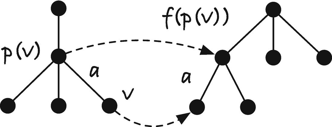
Jumping the failure link of a parent to get the failure link of a child
To set the failure link for node v, we first exploit that the parent of the node will have a failure link, so we can jump to the node it points to, f (p(v)). If we can find an out edge there that matches a, then the node at the end of the out edge will be v’s failure link. We have the longest suffix of p(v) that is in the trie, and we must have a suffix of p(v) as the initial sequence to the failure link of v, f (v). If we can extend it with a, we have the longest suffix of p(v) plus a so the longest suffix of v in the trie; see Figure 2-33. If we cannot extend f (p(v)), then we take the next longest suffix of p(v) in the trie, f ( f (p(v))), and try there, and we continue following failure links until we find one that we can extend. If we handle nodes in a breadth-first manner, we are guaranteed that all nodes closer to the root than v will have their failure link set, so we have f (p(v)) and all fn (p(v)) set since these will be higher in the trie; they are suffixes of p(v) and must, therefore, be shorter strings and thus higher in the trie. If there are no places we can extend, then the only option we have is to set the failure link to the root.
To insert all children of a node, you can call enqueue_siblings() on its first child.
For the output list, observe that we will have to output all the strings in the output link of the failure link of v—those are the strings that are suffixes of v with a string label. If v has a string label we must also output it, so in that case we prepend v’s label to the list; otherwise, we take the output of f (v).
When we examine the running time for the preprocessing, we will assume that the trie is already built; if you want to include it, just add the construction to this running time. Building the trie can be done in time equal to the total sum of the lengths of strings in it, O(m). Constructing the failure links can be done in the same time.
It isn’t obvious that we can construct the failure links in linear time. For each node v at depth d(v), we can in principle follow d(v) failure links, giving us a running time of the square of the number of nodes in the trie. This, however, is not a tight bound. To see this, consider a node v and the path down to it. When we compute the failure links, we do it breadth-first, but for now consider what amounts to a depth-first traversal. If the failure link is set for v and we need to compute it for a child of v, w, then the node depth of f (w) can at most be one more than the node depth of f (v). When we compute f (w), we might decrease the failure depth by a number of steps but we can only increase it by one. As we move down a depth-first path, we can increase the failure link depth by one at each step, but we cannot decrease it more than we have increased it so far. So the total search for suffix links on such a path is bounded by the depth of the path.
The algorithm with iterators
For the running time of the main algorithm, we can reason similarly to how we did for the KMP algorithm. We never decrease j, but we increase it for each match. We never move the trie to the left but move it to the right every time we have a mismatch. Both j and trie cannot move past the end of x, so the running time is (n) plus the total number of matches we output, z, which is not a constant, so the total time is O(n + z).
Comparisons
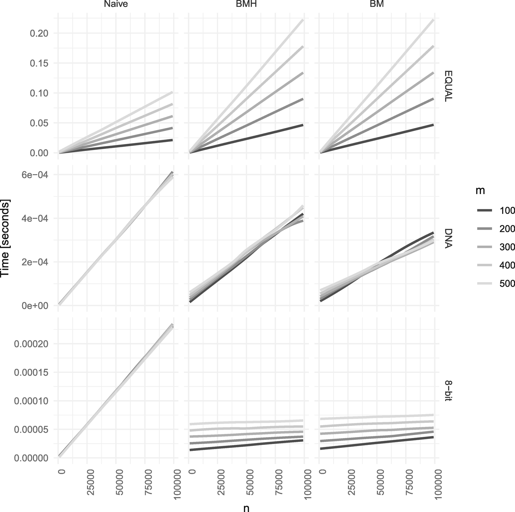
Theoretical analysis of algorithms is one thing, and actual running times another—and more important property. I have simulated random strings with three different alphabets: EQUAL, all symbols are the same; DNA, an alphabet of size four (A, C, G, T); and a full 8-bit character set. If our analysis (and implementation) is correct, the naïve algorithms, BMH and BM, should have worst-case complexity on EQUAL, but when we consider random strings, the performance should get better the larger the alphabet. The other algorithms should run in linear time regardless of the alphabet. The relative performance of the two classes of algorithms depends on the complexity of the implementation. So consider Figure 2-34. In the figure, I have used m = 200. The lines are loess fitted to the time measurements. The behavior is as expected: The first three algorithms perform poorly with the EQUAL alphabet but comparable to the other algorithms on the DNA alphabet. The naïve algorithm is a little faster because it is much simpler. With random strings, the BMH and BM algorithms outcompete the others, with BM (the more complex of the two) the fastest. With the largest alphabet, the naïve algorithm, simple as it is, is faster than border and KMP, and the BMH and BM algorithms dramatically faster.
The algorithms also depend on m, and in Figure 2-35, you can see the running time of the linear-time algorithms for different m. In Figure 2-36 you can see the same for the worst-case quadratic time algorithms. Notice that the linear-time algorithms hardly depend on m. There is some dependency from the preprocessing step, but it is very minor. The worst-case quadratic time algorithms depend on both n and m. When we fix m, we always get a straight line for O(nm) algorithms, but the growth depends on m as we see. They are all faster for smaller m and faster for larger alphabets (the y axes are not on the same scale so you can see the running time for the fastest cases).
You are unlikely to run into truly random strings, but genomic DNA data is close enough that the running time will be the same. Natural languages are hardly random, but BMH and BM are known to perform sublinear there as well. The best algorithm depends on your use case, but with reasonably large alphabets, BM and BMH are likely to be good choices.

Performance of the search algorithms

Dependency on m for the linear algorithms
Performance of the worst-case quadratic time algorithms for different m