
The suffix tree is a fundamental data structure when it comes to string algorithms. It captures the structure of a string via all the string’s suffixes and uses this structure as the basis of many algorithms. We will only use it for searching, where it provides linear search for a pattern after a linear preprocessing of the string we search in.

Suffix trie for “mississippi”
Constructing this “suffix trie” in the standard way—one string at a time—takes time proportional to the sum of the lengths of sequences we add to the trie, so building this suffix trie costs us O(n2) space and time usage for the preprocessing. A suffix tree is a tree containing all suffixes of a string but exploits the structure in a set of suffixes to reduce both space and time complexity to O(n + m).
Compacted trie and suffix representation

Suffix tree, conceptual and actual
The sentinel guarantees that there is a one-to-one correspondence between the string’s suffixes and the suffix tree’s leaves. Since each inner node has at least two children, the total number of nodes cannot exceed 2n − 1 and neither can the number of edges, so the suffix tree can be stored in O(n) space.
The range_length() is a convenience function and shows how we can go from pointers to a length, and in this case, it will be an offset from the string pointed to by r.to.
In the simplest construction algorithm, we need a range, a sibling list, and a child list in each node, plus a suffix label if the node is a leaf. In the more advanced two algorithms, we also need a parent pointer and a suffix link pointer. What the parent pointer does should be self-evident, and the suffix link pointer will be explained when we get to McCreight’s algorithm later in the chapter.
The edge_length() function is just another helper function we can use to, not surprisingly, get the length of the edge leading to the node.
This function should remain in the .c file and not be part of the public interface. We don’t want the user to insert nodes willy-nilly. Suffix trees should be built using a construction algorithm.
We should not free the string when we free the suffix tree. That is the responsibility of the user and part of the interface; the string is declared const, and we will use const strings for all our construction algorithms.
Naïve construction algorithm
First, we ensure that there is at least one edge out of the root—otherwise, we would need to handle the case where, and there isn’t a special case in all the other functions we will write. After setting the first suffix as the first child of the root (and setting the parent pointer of it to the root), we iterate through all the remaining suffixes and insert them using the following naive_insert() function . This function will return the new leaf representing the suffix, and we set its label accordingly.
The naive_insert() function takes the suffix tree, a node to search out from (the root in naive_suffix_tree() ), and a string given by a start pointer (x + i for the start of suffix i) and an end pointer (the end of the string in naive_suffix_tree().
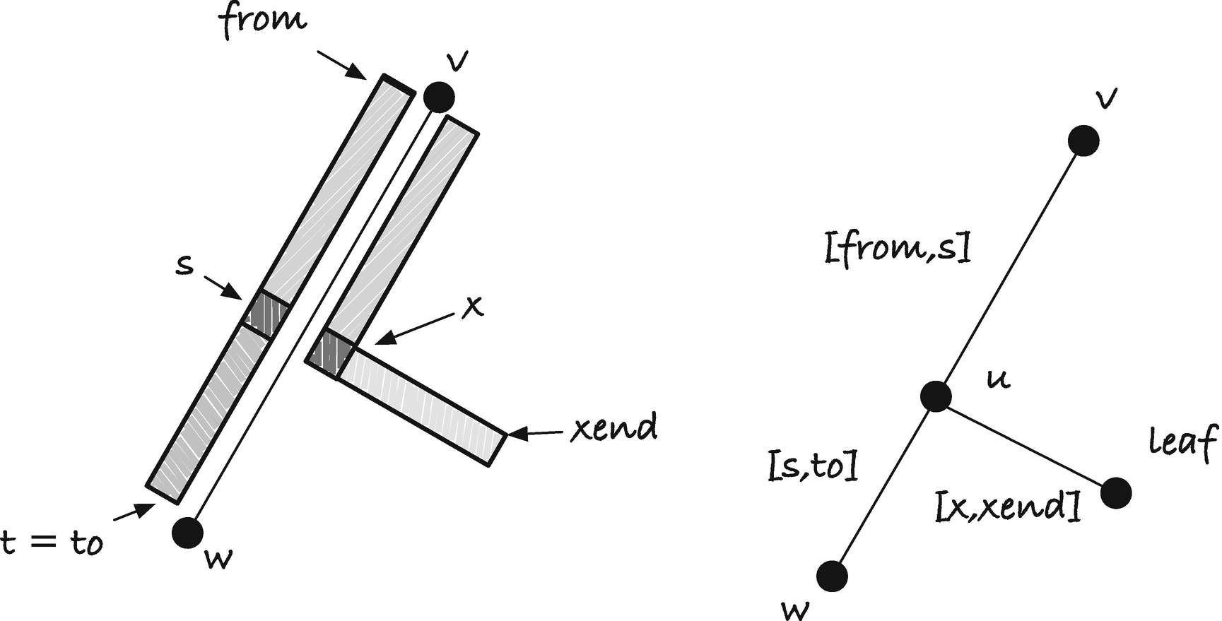
First, naive_insert() checks if there is an out edge from the node it should search from, v. If there isn’t, then this is where we should add the string, so we create a new node and insert it as a child of v using insert_child() (listed in following code). If there is an out edge, we scan along it. We get a pointer to the start of the interval of the edge, s, and we have the pointer x pointing to the beginning of the string we want to insert. We scan along the edge as long as s and x point to the same character; see Figure 3-3 for an illustration of how scanning an edge maps to scanning an interval in the suffix tree’s string. In the figure, variables from and to define the interval of the edge we scan, s the point in the edge we have scanned to, x the position in the string we insert that we have scanned so far, and xend the end of the string we are inserting.

Scanning along an edge by scanning in the string
Splitting an edge

Suffix array and longest common prefix array
Suffix trees and the SA and LCP arrays
In this section, we briefly cover the close relationship between two special arrays and a suffix tree. These arrays are the topic of the entire next chapter, but in this section, we only consider how we can use them to build a suffix tree. If you take a list of all the suffixes of a string and then sort them (see Figure 3-5), the suffix array (SA) is the suffix indices in this sorted order. The longest common prefix (LCP) array is the longest prefix of a suffix and the suffix above it in the sorted order—the underlined prefixes in Figure 3-5. In this section, we shall see that we can construct the arrays from a suffix tree in linear time and that we can construct the suffix tree from the two arrays in linear time.
Constructing the SA and LCP arrays
If we depth-first traverse a suffix tree with children sorted alphabetically, we will see all leaves in sorted order, an observation that should be immediately obvious. Thus, if we keep a counter of how many leaves we have seen so far and use it to index into the suffix array, we can build the suffix array simply by putting leaf nodes at the index of the counter as we traverse the tree.
Getting the LCP array is only slightly more involved. If we let branch length be the total length of the string, we read from the root down to a node v. All children of v will share a prefix of exactly this length, so if we iterate through all but the first child, we will have at least this longest common prefix. Children of the children will share longer prefixes, but we can handle that by recursion. The problem with the first child is that though it shares the prefix with the other children, it does not share it with the previous string in the suffix array.
Consider Figure 3-6. The letters represent branch lengths and the numbers the leaves in the tree. Notice how the leftmost node in any of the subtrees has a lower LCP than its siblings. If we traverse the tree and keep track of how much we share to the left, we can output that number for each leaf. For the first child of a node, we send this left-shared number unchanged down the tree, while at the remaining trees, we update the value by adding the edge length of the children’s parent node.
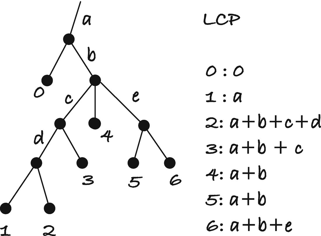
Branch lengths and LCP array
Since the entire algorithm is a depth-first traversal where we do constant time work at each node, the running time is the same as the size of the tree, so O(n).
Constructing the suffix tree from the SA and LCP arrays
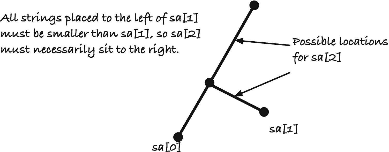
Possible placements of sa[2]
We first add sa[0] to the tree and set the variable v to the new leaf. Then we iteratively add the remaining leaves with lcp_insert() that returns the new leaf inserted. This leaf is used by the function as the starting point for inserting the next leaf.
For the function doing the hard labor, lcp_insert(), consider Figure 3-8. If we are at the leaf for sa[i-1] and the longest prefix it shares with sa[i] is lcp[i], then the new leaf should be inserted lcp[i] symbols down the path from the root to sa[i-1], or n-sa[i-1]-lcp[i] up from the sa[i-1] leaf. We can search up that amount from sa[i-1] and break the edge there (or insert the new leaf in a node if we do not hit an edge).
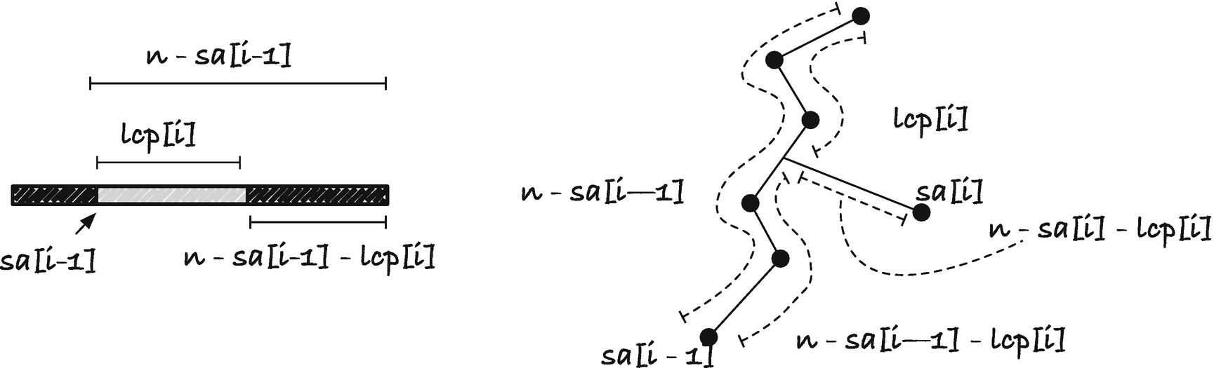
Relationship between sa[i-1], lcp[i], and the suffix tree

Splitting the edge when inserting sa[i]
To see that the running time is linear, observe that we construct the tree in what is essentially a depth-first traversal. We do not traverse nodes going down the recursion—that only makes the running time faster—but each time we move up the tree, it corresponds to returning from the recursion in the traversal. If this is not clear, I encourage you to work out a few examples on a piece of paper until you see that this is the case.
An alternative argument for the running time uses an amortization argument, not unlike those we used for, for example, border arrays, KMP, and Aho-Corasick. Consider the depth of the leaf we start an iteration from, v with node depth d(v). The node depth d(v) is the number of nodes on the path from node v to the root. When we search upward, we decrease the depth, but we cannot decrease it more than d(v). After we find the node or edge, we potentially increase the depth of all the nodes lexicographically smaller than the suffix we are inserting (when we split an edge), or we leave them alone (when we insert a child to node). However, we will never explore that part of the tree when we insert lexicographically larger suffixes. We will look at nodes and edges closer to the root than that point, but we will never return to that subtree since we will never insert a lexicographically smaller string in the algorithm. So we can ignore those increases in depth and only consider the increase when we insert a new leaf. That increase is at most one. The algorithm can at max increase the depth by one (for the relevant part of the tree) in each iteration, and we cannot decrease the depth more than we have increased it, so since there are O(n) leaves in the tree, we have a linear running time.
If we use the SA and LCP arrays to build the suffix tree, and need a suffix tree to produce the arrays, we have a circular problem. We shall see in the next chapter, however, that we can build the arrays in linear time without using a suffix tree. We shall also see, in the next section, that we can build a suffix tree in linear time without the two arrays. A benefit of using the SA and LCP algorithm to construct suffix trees is that it will be easier to preprocess a string using a suffix tree and then serialize it to a file when you expect many searches in the same string over time. The two arrays are trivial to write to a string, while serializing the tree structure itself means saving a structure with pointers and reconstruct them when the tree is read from file.
McCreight’s algorithm
McCreight’s algorithm lets us construct suffix trees in linear time without any additional data structure beyond the string itself. It inserts suffixes in the order they appear in the string, x[0, n]$, x[1, n]$, …, $, just like the naïve algorithm, except that it inserts the next suffix faster than the naïve algorithm. It keeps track of the last leaf inserted, like the SA and LCP algorithm, but the two tricks it uses to achieve linear construction time are different. From the latest leaf that we insert, we use a pointer to jump to a subtree somewhere else in the tree, where the next leaf should be inserted. Then we search for the insertion point in that tree, first using a search method that is faster than the naïve one and then searching the last piece of the suffix using the slow scanning method from the naïve algorithm.

Inserting suffix i by finding its head and appending its tail
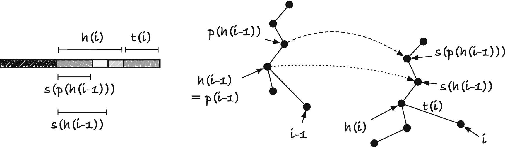
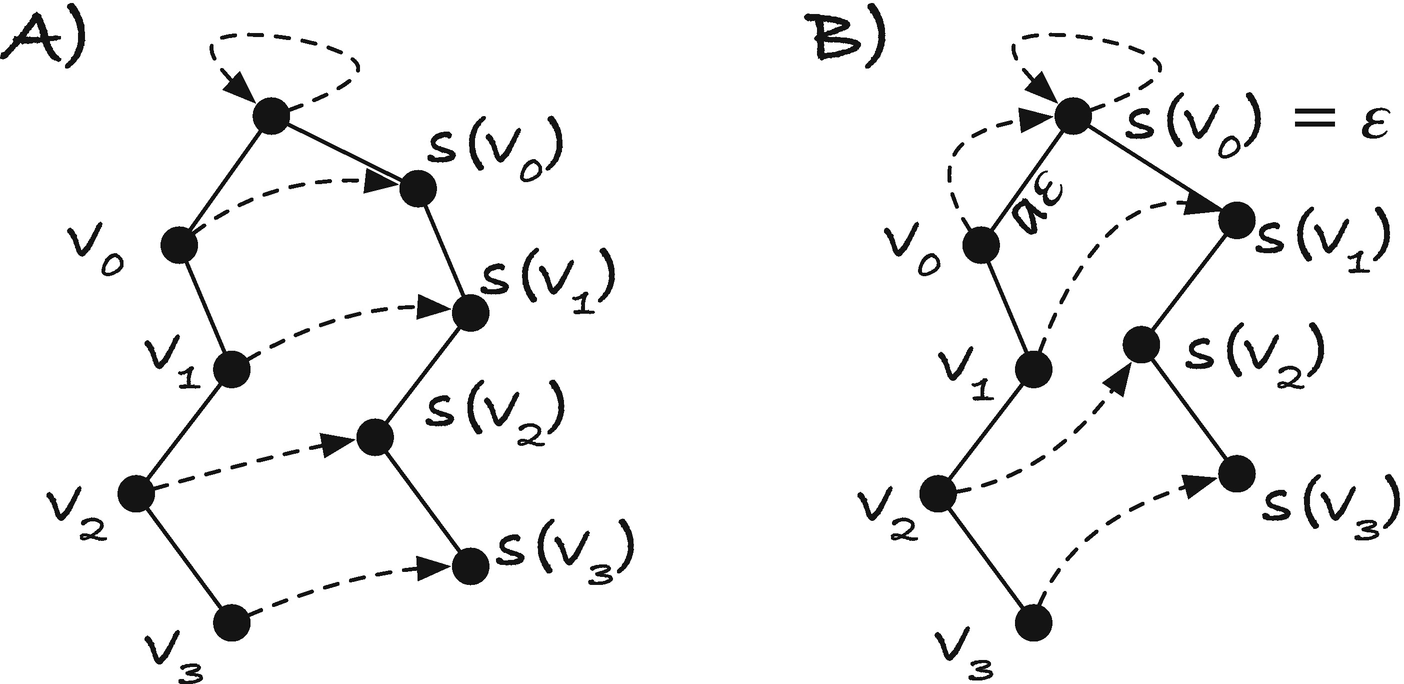
What we did in the naïve algorithm was searching one character by one character from the root to the point where suffix i would branch off the existing tree, that is, we searched for h(i), and then we inserted a new leaf with label t(i). We searched with the naïve search algorithm, one character at a time, and when we could not continue down the tree, we had found h(i). We did not need to insert that string—by definition, it is already in the tree—but we needed a new leaf and the remaining part of the suffix, t(i), on the edge to the leaf; see Figure 3-10. In McCreight’s algorithm, we do essentially the same, but we exploit the structure of suffixes to search for h(i) faster.

The head of a suffix is longer to or equal to the previous suffix’ suffix link
First, observe that s(h(i − 1)) is a prefix of h(i). Consider h(i − 1). This string is how far down the tree we could scan before we found a mismatch when we inserted suffix i − 1. Therefore there was a longer suffix, k < i − 1, whose prefix matches h(i − 1) and then had a mismatch (there might be strings that match more of suffix i − 1, but by definition, this was the longest at the time we inserted i − 1). Now consider h(i). This is the longest prefix matching a prefix of a string we already inserted in the string. If we look at suffix k + 1, we can see that this will match s(h(i-1)); see Figure 3-11. Because we match at least suffix k + 1 to this point, s(h(i − 1)) must be a prefix of h(i). If we only have suffix k + 1 that matches to this point, then we would have exactly h(i)=s(h(i-1)), but there might be longer strings matching a prefix of suffix i; after all, this suffix starts with a different character, and there might be suffixes that do the same and matches longer prefixes. Regardless, we know that s(h(i-1)) is a prefix of h(i).
Head and suffix links and their “jump pointers”
The overall steps in the algorithm are this: We start by creating the first leaf and connecting it to the root. After that, we go through each suffix in order and get the parent of the last leaf we inserted (h(i − 1) in Figure 3-13 and the code). As an invariant of the algorithm, we will have that all nodes, with the possible exception of h(i − 1), will have a suffix link pointer. This is vacuously true after we have inserted the first leaf. For the root, though, it has a suffix link. We set the root’s suffix link to the root itself in alloc_suffix_tree() , so although we need to set the suffix link when we increment i, to ensure the invariant, it is already satisfied at this point.
Searching for the head of suffix i

Cases for scan 2
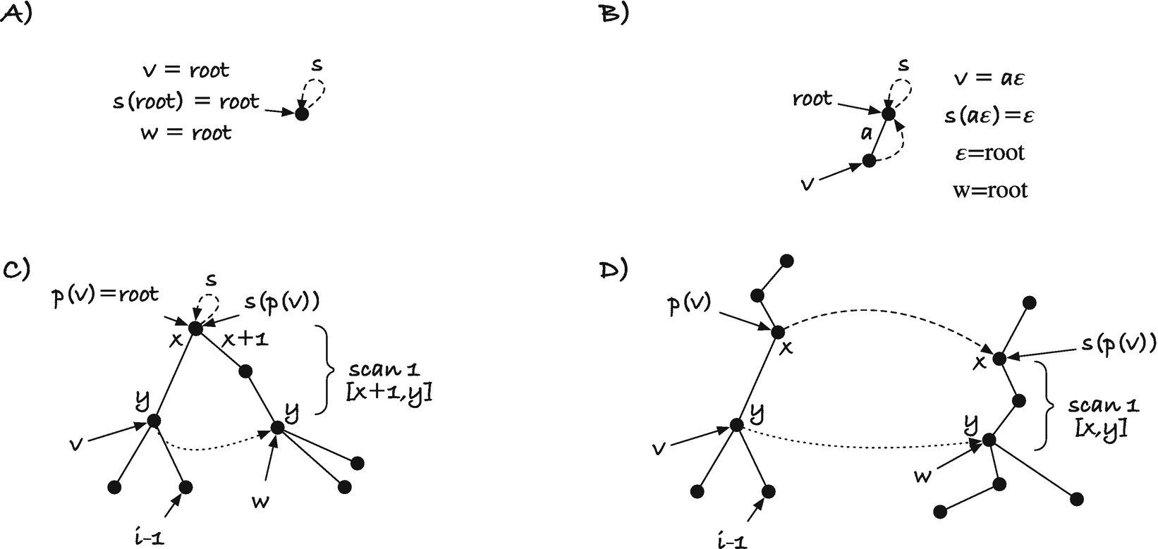
If h(i − 1) is empty (i.e., the root), we cannot search from t(i − 1). The string t(i − 1) is the entire suffix x[i − 1, n]$ (see Figure 3-14 B). We need to scan for the entire suffix x[i, n]$ to find h(i).
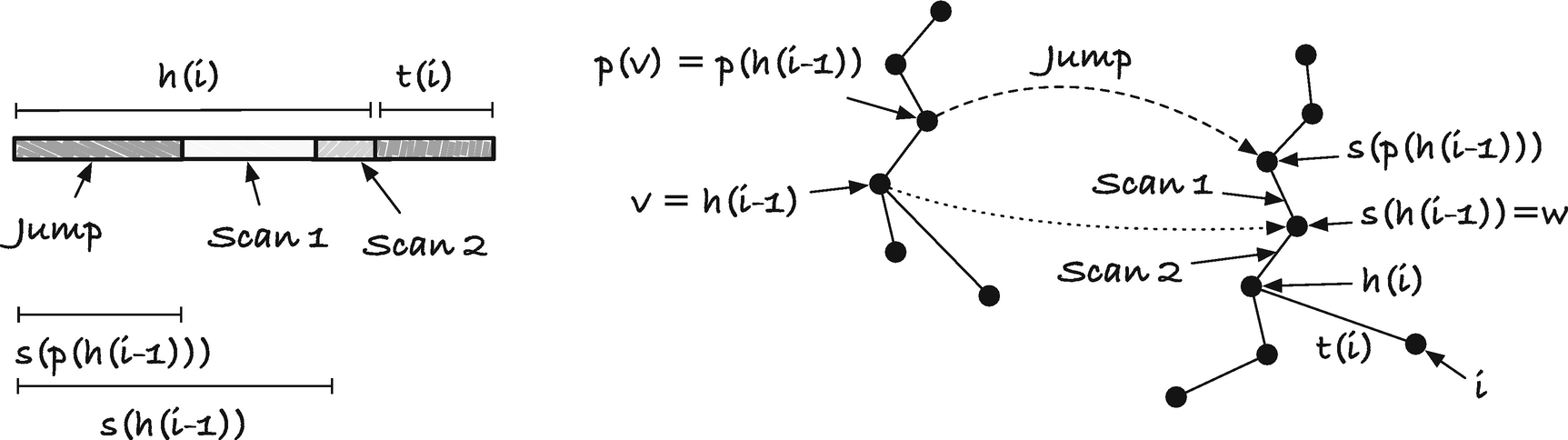
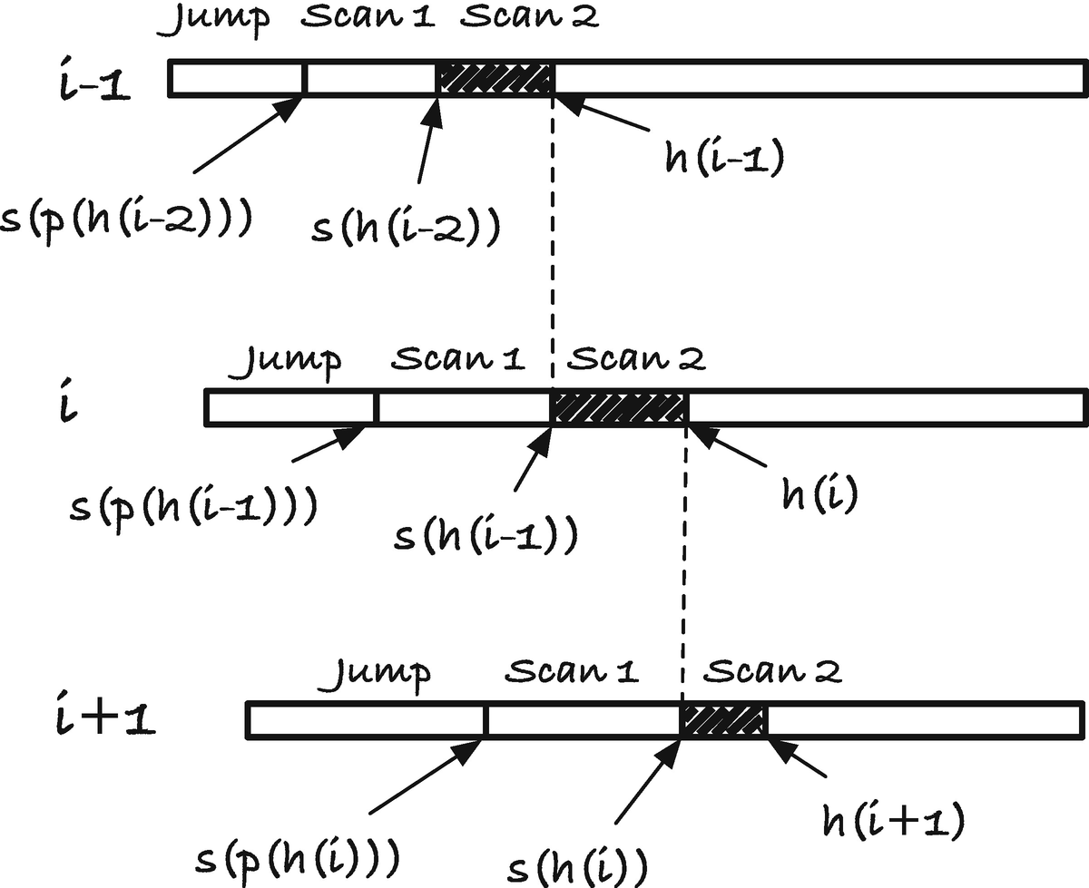
Now, the suffix_search() function is responsible for finding s(v) = w for node v; see Figure 3-13 and Figure 3-15. For this it uses two operations, it goes up to p(v) and then jumps to s(p(v)), and then it searches from there to w in the “scan 1” step. If the edge label on the edge from p(v) to v is the string from x to y (i.e., the pointers in the node representing v have the range from x to y), then it is this string we must search for once we have made the parent and suffix jumps.

General case of suffix search
Four cases for finding the suffix of node v
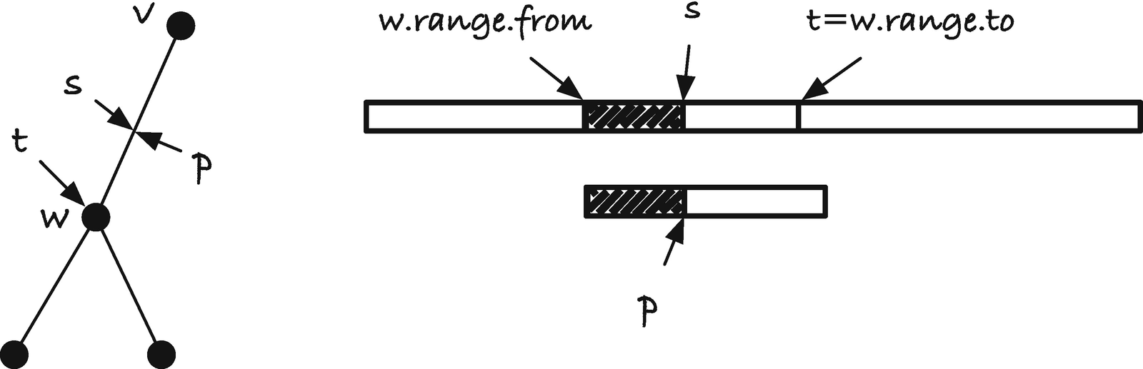
The fast_scan() function handles the “scan 1” part of the algorithm, and as the name suggests, it is faster than the naïve search we use for “scan 2”. We call it with a node and a string range. Call these v, x, and y. We want it to return the node w below v where the path label spells out the string from x to y or create such a node if it doesn’t exist (so we always get a node from a call to the function). It is the same behavior as the naïve search in the tree has, but we will exploit that when we use fast_scan(), we call it with a string that we know is in the tree below node v. It is guaranteed by the observation that s(h(i − 1)) is a prefix of h(i). If we know that a string is in the tree, we do not need to compare every symbol down an edge against it. If we know which edge to follow, we can jump directly from one node to the next. This is what fast_scan() does.3
Let w be the node at the end of the edge where the first letter matches the first symbol we are searching for, and let s and t be the pointers that define the edge label from v to w. Let n be the length of the string, n = t − s, and let z = x + n, that is, z is the point we get to if we move x forward by the length of the v to w edge.
We have three cases for fast_scan(), depending on how the string s to t compares to the string from x to y; see Figure 3-17. (A) The two strings could match exactly. This means that we have found the string we are looking for so we can return w. (B) The string x to y might be shorter than then string from s to t—which we can recognize by z < y. In this case, we need to create a new node for where the x to y string ends and return the new node, node u in the figure. Finally, (C) the x to y string might be longer than the string from s to t. If this is the case, we need to search for the remainder of x to y, the string from z to y, starting in node w and we do this recursively.
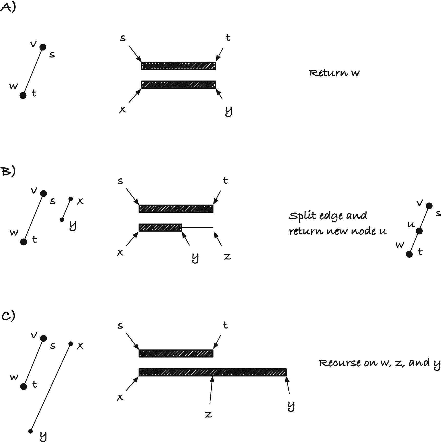
Fast scan cases
The second case in the fast scan, where we split an edge, leaves a node with a single child, violating an invariant of suffix trees. This should worry us, but it isn’t a problem because we immediately after the fast scan search with a naïve insert. This naïve search will see a mismatch on the existing edge and insert t(i) on an out edge of node u, returning us to a tree that satisfies the invariant.
To see that this is the case, see Figure 3-18. By definition, h(i − 1) is the longest prefix of suffix i − 1 before we have a mismatch, so there must be some longer suffix, k < i − 1, that shares prefix h(i − 1) and then mismatches. Let the symbol at the mismatch be a for suffix i − 1 and b for suffix k. When we insert suffix i, suffix k + 1 must have been inserted. Suffixes k + 1 and i share the prefix s(h(i − 1)) and the next character in k + 1 after s(h(i − 1)) is b, and since we broke a single edge, so there is only one symbol that continues from this point, we must conclude that the symbol after the point where we broke the edge must be b. Since t(i − 1)—which is the string we will search for in after calling fast_scan()—begins with symbol a, we will get a mismatch immediately and conclude that s(h(i − 1)) is indeed h(i).
To analyze the running time of McCreight’s algorithm, we split it into three parts: (1) The total work we do when jumping to parent and then the suffix of the parent, (2) the total work we do when using fast_scan() to handle “scan 1”, and (3) the total work we do with naive_insert() to handle “scan 2”.
Of the three, (1) is easy to handle. For each leaf we insert, of which there are n, we move along two pointers which take constant time, so (1) takes time O(n).

Splitting an edge in fast scan
Relationship between a path and the path of suffix links

Uniqueness of suffix links
In each iteration of (2), the pointer jumps, thus decreasing the depth by at most two; after which “scan 1” (or fast scan) increases the depth by a number of nodes. It cannot, however, increase the depth by more than O(n)—there simply aren’t paths long enough. In total, it can increase the depth by O(n) plus the number of decreases in the algorithm which is bounded by O(n). In total, the time we spend on (B) is linear.
Slow scan (scan 2) time usage
Searching with suffix trees
To search for a pattern p in a suffix tree of a string x, we use the strategy from the naïve insert we have seen before. We scan down edges in the tree until we either find the pattern or find a mismatch. If the first is the case, then the leaf of the subtree under the edge or the node where we had the hit will be the positions in x where p occurs. The function below implements it. Here the pattern is null-terminated, as C strings are, but do not confuse this null with the sentinel in x$. If we reach the end of the string, we have a null character, and that is how it is used. The function doesn’t directly give us the positions where the pattern matches. It gives us the smallest subtree where the pattern matches the path label to it. All leaves in this subtree are positions where the pattern can be found in x.
Scanning along an edge when searching for a pattern
Leaf iterators
It is not hard to implement a depth-first traversal of a tree to extract the indices where we have matches, but for a user, iterators are easier to use, which was also our rationale for using them in the matching algorithms in the last chapter. Iterators can be hard to implement, but it is worth it to make the code more usable. An iterator for a depth-first traversal is more complex than the ones we saw in the last chapter, however, because a depth-first traversal is recursive in nature which means that we need a stack, and for an iterator, we need an explicit stack. An explicit stack also solves another problem. A recursive traversal of the tree can have a deep recursion stack and might exceed the available stack space.
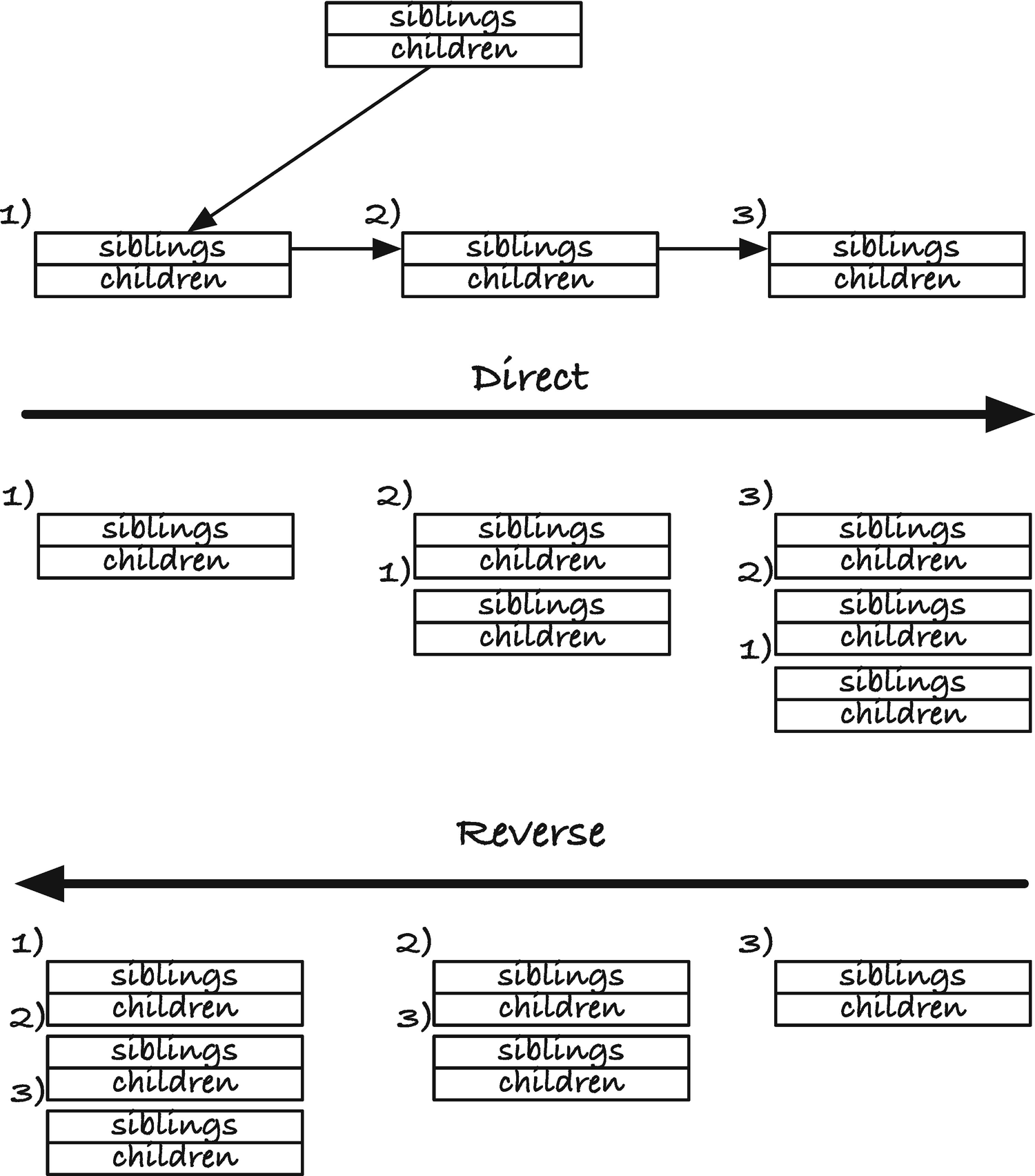
Pushing children, direct or reversed
Comparisons
The naïve implementation runs in worst-case O(n2), while the other two algorithms run in O(n), but how do they compare in practice? The worst input for the naïve algorithm is input where it has to search completely through every suffix to insert it, but for random strings, we expect mismatches early in the suffixes, so here we should get a better running time. It is harder to reason about best- and worst-case data for the other algorithms. For the McCreight’s algorithm, one could argue that it will also benefit from early mismatches since it has a naïve search algorithm as the final step in each iteration. The LCP algorithm doesn’t scan in any way but depends on the SA and LCP arrays (which in turn depends on the string underlying the suffix tree, of course). The algorithm corresponds closely to a depth-first traversal of the suffix tree, so we would expect it to be faster when there are fewer nodes, that is, when the branch-out of the inner nodes is high. We can experiment to see if these intuitive analyses are correct—it turns out that the fan-out of nodes is a key factor and the larger it is, the slower the algorithms get.
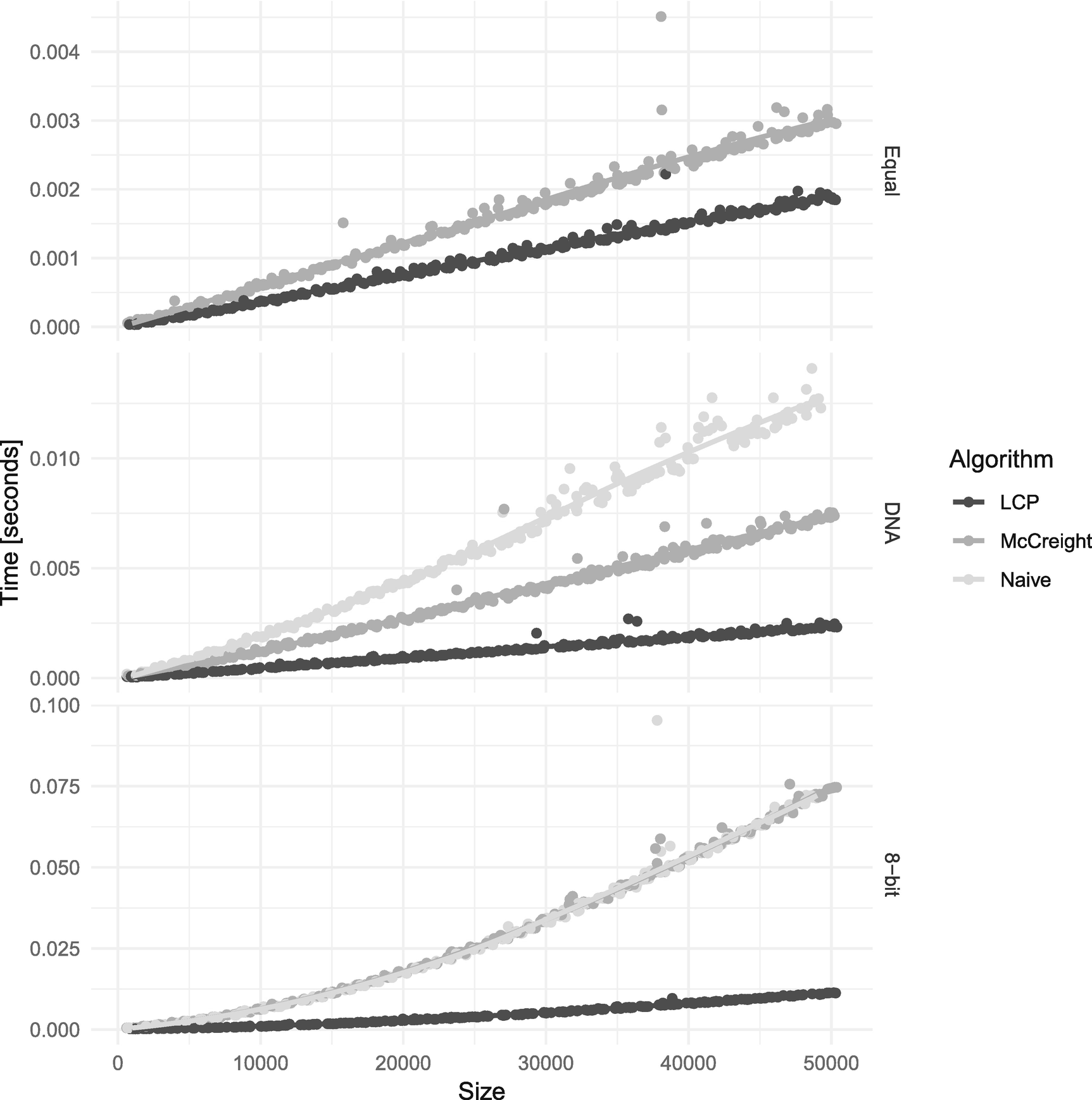
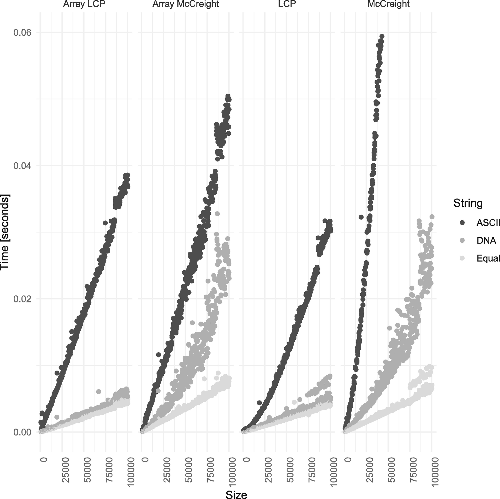
In Figure 3-24 you can see the running time of the three algorithms with three types of strings: Equal, strings consisting only on a single symbol; DNA, random4 sequences over four symbols (A,C,G,T); and 8-bit characters. Figure 3-25 zooms in on the smaller string sizes and leaves out the time measurements for the naïve algorithm on the Equal alphabet.
Some of the results are as we would expect. The naïve algorithm performs very poorly on single-symbol strings but better on random strings. It is still slower than the other two algorithms on random DNA sequences. With the 8-bit alphabet, the naïve and McCreight’s algorithm run equally fast—because mismatches occur faster with a larger alphabet—but notice two things: McCreight’s algorithm is not running in linear time as it should be, and while the two algorithms run in the same time, they are both slower than when we use the two smaller alphabets.

The three algorithms on the three different alphabets
Zoom in on short strings
If the linked lists slow down our algorithm, we can consider an alternative.5 We can use an array for the children, indexed by the alphabet symbols. With this, we can look up the edge for any symbol in constant time. I have shown the running times of the array-based and linked list–based algorithms in Figure 3-26. The array-based algorithms run in linear time and are not affected by the growing linked lists, but they are still affected by the alphabet size. The larger the alphabet, the larger arrays we need to store in each node, and the poorer IO efficiency we will see.
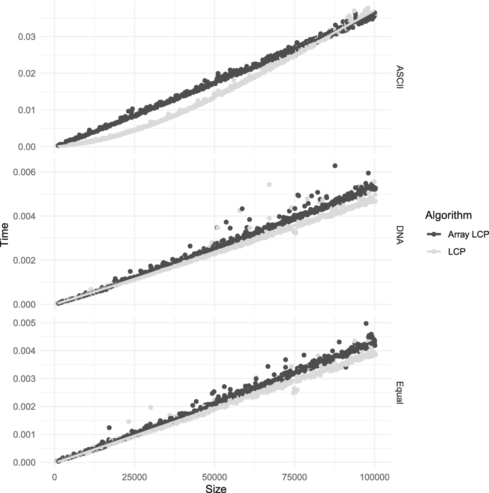
The fastest construction algorithm appears to be the LCP algorithm, linked list or array-based. We can examine their running time in Figure 3-27. The list-based is slightly faster for the smaller alphabets, and for the 8-bit alphabet, it is faster up to around string length 90,000, where the extra memory usage of the array-based implementation pays off. For smaller alphabets, it seems that the LCP algorithm with linked lists is the way to go.
Array-based children
Array- and list-based LCP constructions
Adding the array computations to LCP
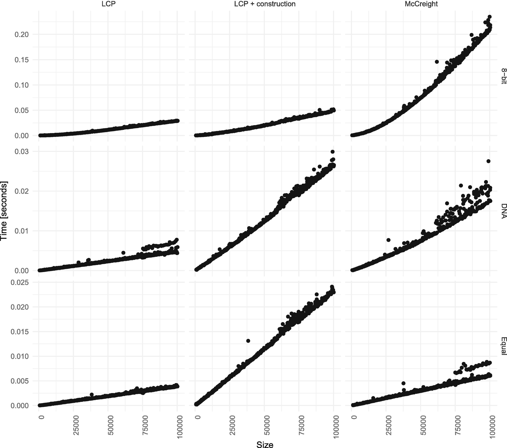
If we do not have the arrays precomputed, then McCreight’s algorithm or even the naïve algorithm is competitive. The naïve algorithm is, obviously, only worth considering with a large alphabet, but its simplicity and a running time compatible with McCreight might make it a good choice. Further, if memory is a problem, and each word counts, you can implement it without the parent and suffix link pointer; McCreight needs both (and LCP needs the parent pointer but not the suffix link).
You can find the code I used for the measurements on GitHub: https://github.com/mailund/stralg/blob/master/performance/suffix_tree_construction.c.