The first stage in translating the essential model into a picture of the desired implementation is to identify the processors that will carry out the work of the system. It is then possible to reorganize the essential model around the processors chosen. The resulting model has the same content as the essential model, and predicts the same system behavior, but has a different upper-level partitioning. Figure 3.1 suggests the difference in organization between the two models. Note that the transformation schema notation is used differently in the two models; in the essential model a transformation may only represent a portion of the work done by the system, while in the processor stage of the implementation model a transformation may also represent a person or machine that carries out part of the work.

Figure 3.1. The reorganization process.

The reorganization can affect the essential model at any level; referring again to Figure 3.1, the transformation T3 has been partitioned into two pieces, and the corresponding specification has been split between two upper-level portions of the processor stage.

In the following sections, we will first examine the criteria for reorganization and then examine the details of the reorganization process.

Reorganization into the processor model results from a comparison of features of a candidate processor to features of the essential model. The simplest case of reorganization involves allocating the entire essential model to a single processor. The criterion in this case is that the candidate processor be capable of carrying out all the work described by the essential model. If there is more than one candidate processor adequate to the job, a selection based on secondary factors (cost, ease of upgrading, and so on) must be made.

In the more general case, the contents of the essential model are to be allocated among a set of candidate processors. The choice of processors may be based on qualitative distinctions, such as the availability in a particular processor of an extended arithmetic instruction set, array processing capability, or the ability to interface to a particular type of peripheral device. The choice may also be based on quantitative distinctions, such as speed, primary memory capacity, or secondary memory capacity. Finally, the choice may be based on some characteristic of the system’s environment. In the case of a surveillance satellite system, for example, the perception/action space might contain elements (surveillance analysts, on-board camera equipment) that are widely separated geographically. Communications bandwidth or communications cost, and size/weight criteria may thus dictate a distribution of function between on-board and ground-based computers.

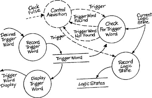
Let’s examine a portion of the essential model for the SILLY system (Appendix C of Volume 2) from the point of view of required speed. The transformations Control Acquisition, Check for Trigger Word, and Record Logic State must be able to operate at the frequency of the Clock Pulse event flow. If the clock pulse occurs at the rate of 1 megahertz, a 1- or 2-MIPS microprocessor could not complete an acquisition cycle rapidly enough to keep pace.

The preceding analysis suggests that a very fast processor is required to do the work described by the essential model. However, the transformations Record Trigger Word and Display Trigger Word need not operate at this fast pace; the speed required is only that of normal keyboard/display processing. Furthermore, the work done by the faster transformations is simple in nature and does not require the capabilities of a general-purpose processor. A reasonable choice might be a pair of processors, a slower general-purpose microprocessor to handle keyboard/display interactions, and a highspeed, special-purpose digital circuit for logic acquisition.

In a multiprocessor allocation, it is possible for the allocation criteria determined by processor characteristics to conflict with the essential model structure. The example of Figure 3.2 does not suffer from this problem; the transformations can cleanly be assigned to either the fast processor or the slow processor. However, this is not true in general.

Figure 3.2. Portion of SILLY essential model.

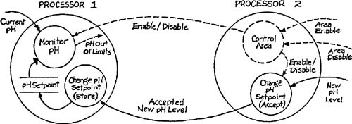
The most serious form of conflict is caused by the need to split a data transformation representing a single event response among two or more processors. Take as an example Figure 3.3, which is extracted from the Bottle-Filling System essential model (Appendix B in Volume 2). When Control Area is enabled, monitoring of pH is active and changing the setpoint is prohibited. When the area is disabled, the reverse is true.

Figure 3.3. Portion of bottle-filling system essential model.

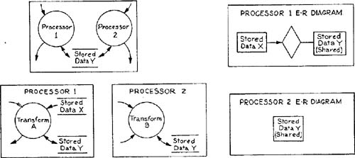
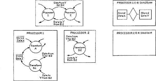
Consider two possible allocations of the Change pH Setpoint transformation: In the first, the pH Setpoint data is shared between two processors, and the acceptance and storage of a New pH Level takes place within a single processor; in the second, the acceptance of the New pH Level takes place in one processor, but the memory and thus the storage activity is localized to a second processor.

The two allocations are illustrated in Figures 3.4 and 3.5. In both cases, there is a synchronization requirement between Change pH Setpoint and the handling of the Area Enable event flow; if the Control Area is disabled and a New pH Level is entered, the data must be placed in storage before an Area Enable is honored. However, in Figure 3.4 the synchronization is entirely confined to Processor 2, provided that Processor 1 isn’t using the shared memory during the period when the area is disabled. In Figure 3.5, the synchronization requires the resources of both processors; once a New pH Level is submitted, the Accepted New pH Level must be both sent and stored before an Area Enable can be honored.

Figure 3.4. Allocation of change pH setpoint to one processor.

Figure 3.5. Allocation of change pH setpoint to one processor.

In addition to the increased synchronization requirement, the allocation shown in Figure 3.5 disperses the logic of an event response between code in two processors. A change to the event response is more difficult to implement in this situation than if the logic were localized to a single processor.

We are not suggesting that allocations like that of Figure 3.5 are always to be avoided. We are suggesting, however, that the costs and benefits of effective use of processor resources versus essential model distortion be taken into account carefully before such decisions are made.

In a complex situation, it is unlikely that the first allocation scheme chosen is likely to be the final one. Allocation should be regarded as an iterative process that allows the visualization and evaluation of alternatives.

As we mentioned in the introduction, processors are represented as high-level transformations on a transformation schema. The name given to a processor should highlight the role played by the processor in the computation rather than its manufacturer, model number, or other physical characteristics. “Temperature Control Micro” is a much more helpful name than “Zip Zap 8000-2Meg” for the purposes of the processor stage of the implementation model.

Another aspect of identification is the distinction between a single piece of hardware and a single processor. As we will use the term in this discussion, we willl identify a single processor from the point of view of the writer of the application code. Consider a configuration consisting of a set of CPUs managed by a multitasking operating system. The operating system activates tasks as required to a “server” (CPU) based on load-leveling considerations. This configuration would be a single processor from the point of view of the implementation model; a coder would be writing code not for a specific CPU but for the entire configuration.

The distinction between a piece of hardware and a processor also applies to the provision of redundant and backup processors for an implementation. The combination of an “active” and a “warm-standby” computer would be represented as a single processor.

Sometimes a decision is made to embed some of a system’s logic within a sensor or actor. This means that the sensor or actor must appear as a processor within the implementation, and can lead to a situation like the one in Figure 3.6. This figure represents a variation on the Bottle-Filling System (Appendix B in Volume 2) in which the pH is provided as a set of values from an array of sensors and must be averaged to obtain current pH. The pH sensor device appears in the overall model twice, as a terminator (source of data) on the essential model context schema and as a processor (manipulator of data) on the implementation model. In Figure 3.6 the essential activity of monitoring the average pH by checking individual sensor values is split between the averaging logic and the pH Control Micro.

Figure 3.6. A sensor acting as both terminator and processor.

People who provide input data to systems often serve as both terminators and as processors by carrying out manual data entry procedures. The inclusion of such manual processors within the processor level provides a convenient vehicle for integrating data entry procedures into the overall system model.

A final consideration on processor identification concerns processors that simply move data from place to place within a multiprocessor configuration. Examples of such processors are message switchers, keyboard handlers, and display handlers. Such processors are often “visible” to the application code only in terms of a low-level call protocol. If this is true, the processor in question should be omitted from the model, since no essential model activities or data are allocated to it.

Now that we have discussed the decision-making processes that lead to allocation, let’s examine the details of the allocation process itself. We’ll first consider the allocation of the transformations from the essential model and their associated specifics.

The allocation of an entire essential model transformation to a processor means that:

The allocation process becomes more complex when a low-level transformation (one described by a specification rather than by a lower-level schema) must be split between two or more processors. Let’s first consider splitting a data transformation. Figure 3.7 shows a transformation from the Defect Inspection System (Appendix D in Volume 2); its associated specification is:

Figure 3.7. A data transformation.

Suppose that this transformation were to be allocated between two processors, an Inspection Surface Micro in possession of the Inspection Surfaces data, and an Operator Console Micro in charge of updating Production Runs and producing the output flow. We will rename the two portions of the original transformation so that we can differentiate the portion of the transformation work that each performs.

The results of the allocation are shown in Figure 3.8. The specification for Change Current Product (I/O) is:

Figure 3.8. Allocation of Figure 3.7.

In general, to split a transformation specification it is necessary to represent the work done by one part of the specification to the other part. The representation may be in terms of data already manipulated by the other part of the specification, or in terms of flags representing the outcome of logic performed by the other part of the specification.

Now that we’ve considered splitting a data transformation, let’s move on to the splitting of a control transformation. Since the specification for a control transformation (the state transition diagram) has a more regular form than the specification for a data transformation, the splitting procedure can be formalized:

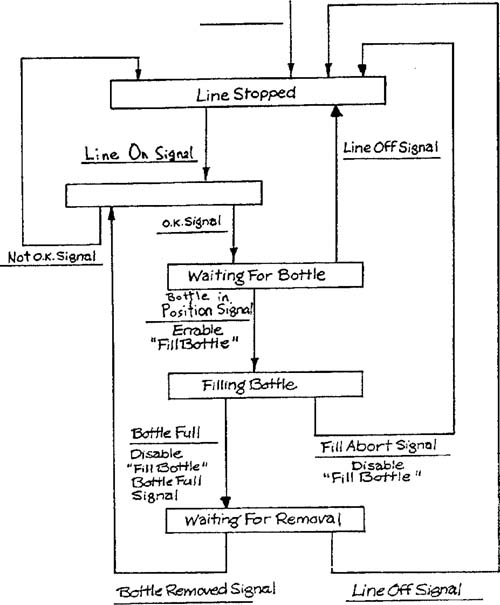
Let’s apply this procedure to the Control Bottling Line transformation from the Bottle-Filling System (Appendix B in Volume 2). The transformation is shown in Figure 3.9 and its associated state transition diagram in Figure 3.10. The transformation will be split between two processors. One (the Fill Control Micro) controls the opening and closing of the Bottle Filling valve and uses the Weight input to determine when the bottle is full. The other (the Mechanical Control Micro) performs the remaining processing (and also has access to the Weight input). Figures 3.11 and 3.12 show the two state transition diagram copies after Step 2 has been applied.

Figure 3.9. Control transformation from bottling system.

Figure 3.10. State transition diagram for Figure 3.9.

Figure 3.11. Fill control micro state transition diagram after step 2.

Figure 3.12. Mechanical control micro state transition diagram after step 2.

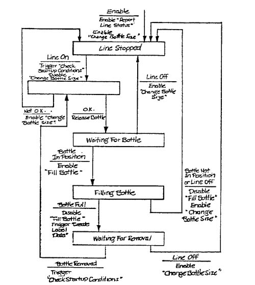
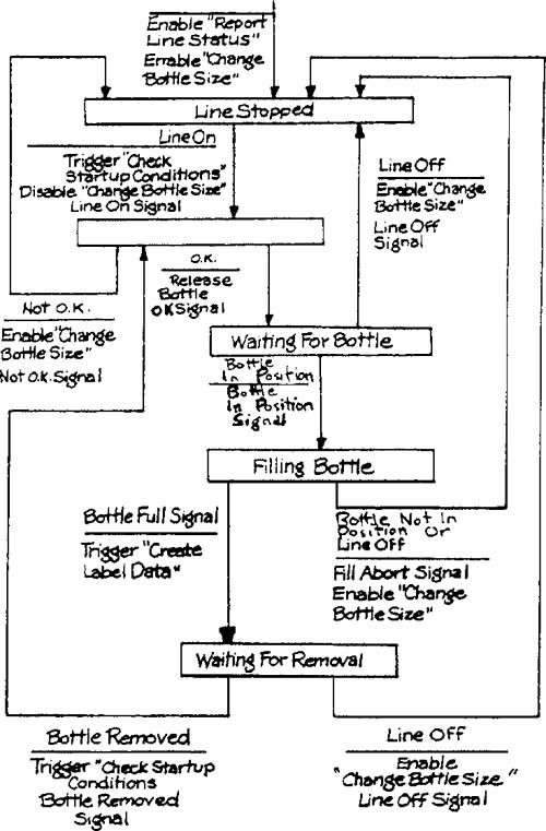
Applying Step 3 to Figure 3.11 results in the removal of the Line Stopped state, the unnamed state, and the Waiting for Removal state. Notice that, if Waiting for Removal is examined first, it cannot be removed because it has two destination states. However, it will be removed on the second iteration since the destination states will have been resolved into a single one.

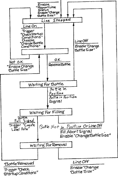
Figures 3.13 and 3.14 show the two state transition diagrams after application of steps 4 and 5. Notice that the ultimate state diagrams satisfy intuitive notions about “which processor needs to know about which state.”

Figure 3.13. Fill control micro state transition diagram — final.

Figure 3.14. Mechanical control micro state transition diagram — final.

Since the stores on the transformation schema correspond to object types and relationships on the entity-relationship diagram, allocating the transformation schema provides information that is important for the allocation of stored data. For example, if all transformations that use a store are allocated to a single processor, that processor should normally “own” the store.^[*] However, questions of allocation of stored data must be looked at for each individual object type and relationship to assure completeness of the allocation. We therefore recommend using the entity-relationship diagram from the essential model to create an entity-relationship diagram for each candidate processor. There are a number of possible mechanisms for making a collection of stored data available to two (or more) processors; we will consider sharing, exclusive ownership, and duplication, using the abstract representation of Figure 3.15.

Figure 3.15. Portion of essential model to be allocated.

In the case of sharing, a physical data storage mechanism (such as a multiport memory) is accessible to both processors. Although some synchronization is necessary (to prevent both processors from trying to change the same item at the same time) the processors are inherently equal in their ownership of the data. A distributed database manager or a database backend processor, both of which make ownership of the data invisible to the application, would also be modeled as sharing. Figure 3.16 shows sharing of stored data between two processors from the point of view of the leveled transformation schema for the implementation model, and from the point of view of the entity-relationship diagrams for the two processors.

Figure 3.16. Sharing of stored data between twp processors.

In the case of exclusive ownership, only one processor has access to the physical data storage mechanism. Therefore the other processor can obtain or modify data only by the cooperation of two processes, one in each processor, that transfer and receive the data. This means that if a transformation does its work in one processor but needs data owned by another processor, the piece of the transformation that actually accesses storage must be allocated to the other processor. The modeling of this situation is shown in Figure 3.17. Note that no details of the data transfer mechanism are shown; the topic will be taken up in Chapter 5, Interface Modeling.

Figure 3.17. Exclusive ownership of stored data by one processor.

Finally, in the case of duplication, each processor has access to a data storage mechanism containing a copy of the data. Each processor can therefore obtain stored data without the cooperation of the other processor. However, a processor can only change stored data with the cooperation of the other processor, since consistency of the duplicate copies must be maintained. If a transformation does its work in one processor but changes data duplicated between its processor and another, a piece of the transformation must be allocated to the other processor to maintain correspondence. The modeling of this situation is shown in Figure 3.18. If the duplication is not exact (some data elements are stored in only one processor) the names of the stores/object types and their associated specifics should be modified to reflect the distinction.

Figure 3.18. Duplication of stored data by one processor.

We recommend carrying out the allocation process by working top-down through the leveled essential model. At each level of the model, each transformation can be checked to see if it can be allocated to a single processor in its entirety. If so, the transformation can be “tagged” as belonging to that processor, and the lower levels of that transformation need not be examined further. If a lowest-level transformation is reached that cannot be allocated as a unit, the transformation must be split, as described in Section 3.4, and the pieces tagged appropriately.

After the transformations are allocated, the stored data should be allocated as described in Section 3.5. Stores and object types/relationships should be tagged for processor ownership. Any transformations that must be split because of data ownership decisions should be modified and tagged accordingly.

When the tagging is complete, the processor stage of the implementation model can be constructed. A screen storage area (or a sheet of paper if the transformation schemas are not stored in a development support machine) should be reserved for each candidate processor. The tagged portions of the essential model should then be copied into the areas for the processors, and joined along common flows and stores. The result of this procedure is a set of transformation schemas, one for each candidate processor.

The transformation schemas created by the allocation procedure may now be integrated into a leveled model.

The upper levels of this model can be created by building a transformation schema with one transformation per processor. The input and output flows and stores for the transformations are the net inputs and outputs from the lower-level schemas. If there are a large number of processors, more than one higher level may be necessary, with some highest-level transformations representing groups of related processors.

The lower levels of the model are created by copying over the corresponding lower-level portions of the essential model (lower-level transformation schemas and transformation specifications).

Since the leveling scheme is different for the implementation model than it was for the essential model, the numbers assigned to transformations will differ between the two models. We recommend creating a cross-reference so that individual transformations can be traced from one model to another. This subject is treated in more detail in Chapter 12, Implementation Model Traceability.

It is important to verify that the processor stage of the implementation model is a complete and correct mapping of the essential model onto the processor configuration. One obvious mechanical verification is to check that all elements of the essential model have been assigned to one of the candidate processors. Another verification is to create a scenario for execution of the essential model, as described in Chapter 9 of Volume 1, Executing the Transformation Schema. A necessary condition for correctness of the implementation model is that execution of the scenario produce the same result as for the essential model.

The processor stage of the implementation model is created by reorganizing the content of the essential model to reflect the choice of a processor configuration. We have described the criteria for processor choice and the mechanics of the reorganization. Note that the portion of the essential model assigned to a processor has no special internal organization. We will take up this level of organization in the next chapter.