The processor model provides a specification of the transformations and stored data assigned to each processor used to implement a system. It is now necessary to reorganize and elaborate the model to adapt it to the internal organization of each processor. This step corresponds to the second stage of the implementation model — the task stage.

The processor model may prescribe the use of any type of processor, and thus portions of the model may be implemented not only as software but also as hard-wired circuits or even as manual procedures. Since we must now account for their internal organization, we must begin to distinguish between different types of processors. In this chapter, we shall focus our attention on programmable digital computers and thus on software implementations.

Each manufacturer of digital computers has developed its own vocabulary to describe the internal organization of the units of software within their processors, and there is therefore little standardization of the terminology. Since we shall be using some nomenclature that is in use elsewhere, it is important to distinguish between our general use of the term task and the specific use to which it is put on particular systems. We define a task as any named, independently schedulable piece of software that implements some portion of the transformation work assigned to a processor. Several vendors use the term more restrictively, for example to exclude software units like interrupt handlers.

In this chapter, we discuss the application of the implementation modeling heuristics to construct a model that describes the organization of software within digital computers.

The task is the basic unit of activity of a processor. We require that a lowest-level task be sequential, and thus concurrency is prohibited within the lowest level of tasks described by an implementation model. However, a group of potentially concurrent tasks can be aggregated into a single higher-level task. For the remainder of the chapter, we will use “task” to mean a lowest-level task unless otherwise noted. Tasks may be truly concurrent with each other if they run on different processors, or on a multi-processor capable of running several tasks simultaneously. In implementations that require more concurrent tasks than there are processors, a processor can simulate concurrency by switching between tasks so that an external observer is unable to distinguish the processor’s behavior from several processors (or a multiprocessor) running concurrently.

Each task may be enabled or disabled, interrupted, and resumed. We define the terms enabled and disabled in the same way as when we discussed transformations in Chapter 6 of Volume 1 — Modeling Transformations. That is, when a task is enabled it is able to accept input and produce outputs, and when a task is disabled it cannot accept inputs nor produce outputs. From the point of view of a run-time operating system, a disabled task does not exist.

Real tasks take time, unlike transformations on the essential model. It is possible for a task to be interrupted and resumed after it has been enabled to allow other tasks to make use of execution resources. The system software of the processor will switch between several enabled tasks by interrupting one task and resuming another, often making choices in terms of a priority ordering for the tasks. The system software keeps data about the operation of the task, called the context of the task. When the system software is switching between one task and another, no useful application work is being done, but the processor is said to be context switching. The time it takes the processor to carry out this activity is the context switching time. The system software can manage the scheduling of tasks by allowing tasks to run while other tasks are waiting for completion of input/output operations by peripheral devices. Another management strategy is time-slicing, giving each task some fraction of the available time.

It is often useful to partition the “enabled” quality of a task into further distinguishing states of the task as follows:

Please note that a task that executes a request for input or output but then continues to carry out useful work is running.

We now move on to describe how a portion of an implementation model to be implemented as software on a single processor may be allocated to a set of tasks.

Chapter 3, Processor Modeling, described the first stage of implementation modeling as reorganizing the essential model around a set of candidate processors. Task modeling can be similarly described as a reorganization of portions of the essential model around a set of candidate tasks. The portions of the essential model referred to are those that were allocated to individual processors during the processor modeling stage.

An allocation to processors does not change the content of an essential model, but simply redistributes the content. Neither does processor allocation centralize control nor restrict any potential concurrency described by the essential model. The number of control transformations is at least as large as in the essential model, and any potentially concurrent transformation in the essential model remains potentially concurrent in the allocated model. The lack of restriction reflects the fact that concurrency and decentralized control can occur among a set of interacting processors, and also among a set of tasks within a multitasking processor.

Allocating portions of a model to a single task changes this situation, since control must be centralized and concurrency is prohibited within a (lowest-level) task. Task allocation will therefore involve modifications of the model to combine control transformations and their associated state diagrams, and to impose sequences on potentially concurrent data transformations.

Combining of a pair of state diagrams is the inverse of the procedure described in Section 3.4 of the last chapter:

Step 1. Add an “undefined” state to any state transition diagram that is enabled by another. Make the undefined state the initial state, and connect it to the transition to the original initial state with a condition of “enable.” Add transitions from all other states to the undefined state with conditions of “disable” and actions to deactivate any transformations activated within the diagram.

Step 2. Begin a new state diagram by creating a state that combines the initial (constituent) states of the two original diagrams. This will be referred to as the combined state.

Step 3. For each condition external to both original diagrams and causing a transition from either of the constituent states and not already dealt with, construct a transition from the combined state and reproduce the condition and the actions from the original transition. Replace any action that sends an event flow to one of the original diagrams with the actions triggered by that event flow.

Step 4. If the external condition from Step 3 causes transitions in both original diagrams, construct a new combined state from the destination states of the original diagrams if distinct from all states already created, and draw the transition to it. Otherwise, construct a new combined state from the destination state of the original diagram with the transition and the current constituent state of the other original diagram, if distinct from all states already created, and draw the transition to it. If the destination state for the condition is a combined state created in an earlier step, draw the transition to it.

Step 5. Repeat steps 3 and 4 for any new combined state created in step 4.

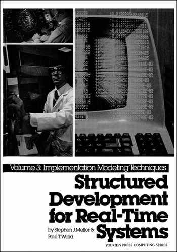
Let’s apply this procedure to an example drawn from the Cruise Control system essential model, Appendix A of Volume 2. Figure 4.1 shows a fragment of the preliminary transformation schema containing four control transformations; event flows to data transformations have been omitted to simplify the picture. The state-transition diagrams corresponding to transformations 1 and 2 are shown in Figures 4.2 and 4.3. Applying the combination procedure to these two diagrams has the following results:

Figure 4.1. Fragment of preliminary transformation schema.

Figure 4.2. Monitor engine.

Figure 4.3. Control mode of operation.

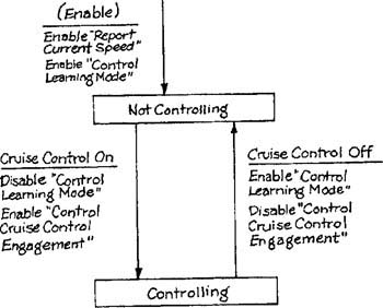
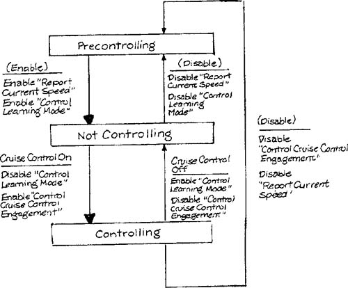
Cycle 1. An “undefined” state called Precontrolling and associated transitions are added to Control Mode of Operation through application of step 1. The resulting diagram is shown in Figure 4.4. Step 2 requires the construction of a state called Engine Stopped/Precontrolling from the initial states of the two original diagrams. The only external condition causing a transition from one of the constituent states is Engine On from Engine Stopped; step 3 requires the corresponding action to be replaced by the action triggered in Control Mode of Operation. Since Engine On causes transitions in both original diagrams, step 4 causes a combined state called Engine Running/Not Controlling to which the transition is drawn. Figure 4.5 shows the new diagram up to this point.

Figure 4.4. Result of applying step 1 to Figure 4.3

Figure 4.5. Combined diagram after cycle 1.

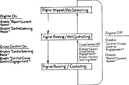
Cycle 2. We return to step 3 and apply the rules to the newly-created Engine Running/Not Controlling state. There are two external conditions from constituent states, Engine Off and Cruise Control On. Engine Off causes transitions in both diagrams and a corresponding replacement of actions. Cruise Control On causes a transition only in Control Mode of Operation. In step 4, Engine Off is seen to cause transitions to Precontrolling and Engine Stopped. Since this combination has already been included in the new diagram, the transition is connected to it. Cruise Control On, on the other hand, causes the creation of an Engine Running/Controlling state from a combination of a new destination state with one of the current constituent states, and the connection of the transition to this new state. Figure 4.6 shows the diagram at the end of cycle 2.

Figure 4.6. Combined diagram after cycle 2.

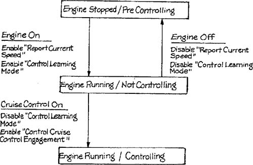
Cycle 3. There are two external conditions causing transitions from the constituents of the new state, namely Engine Off and Cruise Control Off. There are no new state combinations generated, and the results of this final cycle are shown in Figure 4.7. The diagram is consistent with an intuitive conception of the joint effect of the two original diagrams.

Figure 4.7. Final combined state transition diagram.

The reader is invited to refer to the state-transition diagram for Control Learning Mode (transformation 3 from Figure 4.1) in Appendix A of volume 2 and to combine it with the diagram of Figure 4.7. The results are shown in Figure 4.8. Note that the measured mile can be interrupted by turning the cruise control on. This is derivable from tracing the connections among the original three diagrams, but is more clearly seen in the combined diagram.

Figure 4.8. Combination of three state transition diagrams.

The procedure just described centralizes control but does not remove concurrency. State diagrams containing sections like that illustrated in Figure 4.9, in which two data transformations are concurrently enabled, can be allocated to a single task along with the data transformations. In order to ensure that the task is a true sequential process, the model of Figure 4.9 must be modified to prevent A and B from being simultaneously active. Such a modification is shown in general terms in Figure 4.10; the conditions causing transitions among the three states depend on the nature of A and B and will be discussed in later sections of this chapter. Note that the model of Figure 4.10 is not equivalent to the model of Figure 4.9. At best, the model of Figure 4.10 will satisfactorily simulate the model of Figure 4.9.

Figure 4.9. Concurrently enabled data transformations.

Figure 4.10. Sequential approximation of Figure 4.9.

The procedures illustrated in this section, centralization of control and removal of concurrency, underlie all the modeling transformations to be discussed in the remaining sections of this chapter.

An essential model may contain continuous flows and transformations that continuously transform those flows. In an implementation model, such transformations may be allocated to analog processors that are capable of carrying out truly continuous behavior. However, a digital computer may only run discrete tasks, and any continuously operating transformation allocated to a digital computer must be cast into implementable discrete tasks.

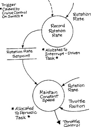
The technique is to allocate the continuously operating transformation to a task that runs periodically; the task samples the continuously available data, processes the data to produce outputs, and is then disabled, to be reenabled after a fixed interval. Any portion of the transformation that operates discretely, such as the computation of a setpoint, must be factored out and executed before the periodic process is activated. For example, Figure 4.11 shows two transformations from the Cruise Control System (Appendix A) that have been allocated to separate tasks. When the driver presses the Cruise Control On switch, the resultant interrupt causes a single activation of Record Rotation Rate, and initiates a periodic activation of Maintain Constant Speed to simulate continuous maintenance. The essential requirement will be satisfactorily approximated if the sampling interval is short enough to resolve the highest frequency variation in the input flow that must be detected [1]. The sampling rate, and therefore the interval, can be computed for each transformation by examining the environmental constraints — specifically, the frequency of variation in the input flow, the specification of the transformation, and the speed at which the external processes under control can respond.

Figure 4.11. Continuous transformation factored into initializing and periodic components.

Each continuously operating transformation could now be allocated to a separate periodic task which runs at the rate necessary to satisfy the environmental constraints imposed on the essential transformation. However, limitations on the number of tasks that may be scheduled to run and the costs of context switching between tasks may lead to a need to group several essential transformations together into a single task. For example, three transformations with required sampling intervals of 40 ms, 50 ms, and 60 ms may all be classified together and allocated to a single task that operates on a 40 ms interval. While this arrangement carries out more processing than is required (the 50 ms and 60 ms fragments are running more frequently than needed), it is nevertheless often necessary since it may be impractical to allocate every transformation to a separate task.

When several concurrent transformations are allocated to a task, concurrency must be removed to accommodate the sequential nature of the task. Figure 4.12, derived from the Bottle-filling System (Appendix B), is a specialization of Figure 4.9 to deal with the issue of allocating continuous transformations. If the Control pH and Control Input Valve transformations are allocated to a single task, the control logic must be modified as shown by Figure 4.13. In this case, the control considerations are relatively simple. The code for performing the pH and input valve control loops can simply be sequenced inside the task. The remainder of the control can be implemented by scheduling the task to run at the necessary interval using the operating system scheduler or a timer, and an essential requirement to disable the transformation can be implemented by requesting the operating system to stop activating the task. The Enable and Disable statements in the essential model are simply replaced by calls to the operating system.

Figure 4.12. Concurrently enabled continuous transformations.

Figure 4.13. Sequential, discrete approximation of Figure 4.11.

The situation becomes more complex when several continuous transformations are allocated to a single periodic task, and the enabling and disabling actions are asynchronous. Each transformation is to be enabled or disabled independently of other transformations allocated to the task; therefore, the control of the transformations cannot be implemented by enabling and disabling the entire task. The periodic task must be activated when the system is initialized, but component portions that correspond to disabled transformations must not run. The flags shown in Figure 4.14 represent control information that states whether each portion is to run. Please note that the control information is represented by a data store, not a control store. (A control store is an essential model variant of a semaphore mechanism.) A task that implements the control transformation is responsible for setting and resetting flags as an implementation of the enabling/disabling logic, as shown in Figure 4.14 drawn from the Cruise Control System. Note that the Speed Control task contains transformations to maintain, increase, and resume speed. Which one is run during an activation is controlled by the flags.

Figure 4.14. A periodic task controlled by flags.

Finally, please note that it is important to retain separation of control transformations from data transformations. Sometimes a continuous transformation that recognizes an event (say a critical temperature value) is allocated to the same periodic task as a continuous transformation (say one that maintains temperature) that is enabled or disabled by the event. If control of the overall state is entrusted to another task, the event recognizer should signal the control task, which in turn will set the appropriate flags. Failure to centralize controlling decisions is an invitation to the introduction of timing problems.

Each of the continuously operating transformations on the processor model may now be allocated to tasks to produce the task model. Several factors affect the choice of tasks:

Consider a collection of continuously operating transformations that must operate at no more than 10 ms, 12 ms, 15 ms, 20 ms, and 35 ms intervals, with a system software organization that is severely limited in the number of tasks it can run simultaneously. A simple solution is to run all the transformations in sequence every 10 ms. This can be a satisfactory approximation of the essential model if the implementation constraints are met, although it wastes execution resources since the 35 ms. transformation is running more often than necessary. Two common failures of this simple solution are, first, that the task takes too long to run, and second, that the task occupies too much memory. We shall examine some variations of the solution that can avoid these failures.

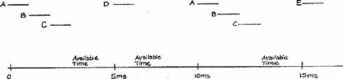
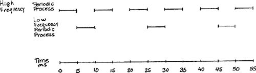
First, if the task takes too long to run, we must take advantage of the fact that not all transformations need to be run every 10 ms; we could, for example, run the task every 5 ms, offsetting the lower-sampling rate transformations by multiples of 5 ms as shown in Table 4.1. The task must keep a count of the pulse number, and run the appropriate transformation only when necessary. (This solution assumes that the first three transformations collectively take less than 5 ms, and each of the last two take less than 5 ms each.) An alternative representation for this organization is a time line, as shown in Figure 4.15. The table, the time line, or an equivalent state diagram specify a control transformation that activates the enabled transformations within the periodic task and that must be modeled in addition to the control transformation that controls the enabling and disabling of the data transformations allocated to the periodic task.

Figure 4.15. A time line.

Figure 4.1. Sampling rate table.

Second, if the task uses too much memory, it must be split into two pieces: one that runs every 10 ms and another than runs every 20 ms, for example. The resulting tasks may either be run offset from one another, say, every 5 ms as shown in Figure 4.16, or they may run at different priorities. This second solution may introduce data consistency problems if the two tasks share data since they may be attempting to modify the same data within the same time interval; a useful technique is to copy shared data into the receiving task at the beginning of each pulse.

Figure 4.16. Time line for tasks with offset.

In a system software organization that permits many tasks to be enabled simultaneously, these complications need not arise since each transformation can be assigned to a separate task. (However, the use of any shared data must be synchronized by spacing out when the tasks run, or by copying the data as described above). In this case, a time line or an equivalent state diagram can act as a specification for a control transformation embodied in the system software for controlling the processor, and it should be supplied as an overall specification for the task level of the implementation model. The details of modeling application-specific aspects of system software are described in Chapter 6 — Modeling System Services — Process Management.

Tasks that incorporate transformations of discrete data must run when the data becomes available. In the previous section, we examined tasks containing transformations of continuous flows in which we chose the rate at which the task was to run, subject to environmental constraints. Here, we do not have the same flexibility, but the principles remain the same: we must satisfactorily approximate the behavior of the essential model with minimum distortion.

In the perfect world of the essential model, we assumed that transformations completed their activities instantaneously; clearly, this does not match the reality. The processing time taken to produce the outputs from inputs must be within the bounds specified by the corresponding constraint; this depends on the speed of access to stored data and the amount of work to be done.

We can have an adequate implementation of a discrete transformation, if the time needed to process an input is within response time constraints, and either:

If the first condition is met, a task containing discrete transformations executes until it requires input, at which point it must idle or pass control back to the processor and enter the waiting for input state. When the input arrives, the task can resume running. Typically, a task of this type will execute a read that sets in motion the activities necessary to get the data. Alternatively the task may idle until the system software sets a flag indicating that data is present.

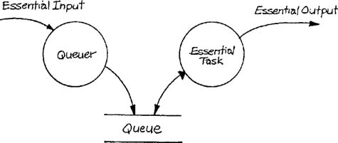
If the data may at times arrive more rapidly than the task can transform the data, then a queuing mechanism can be introduced as shown in Figure 4.17. The addition of a queuing mechanism accomplishes the transformation with two tasks: the essential task (that which actually transforms the data) and an intermediate task that queues the arriving inputs, a queuing task. The control aspects of this model are as follows:

Figure 4.17. Queuer for essential input.

Please note that this scheme is limited by three factors. First, if data arrives faster than the queuer can queue the data then the scheme cannot work. Second, if the queue can hold n data items, and n + 1 items arrive within a time shorter than that required to transform a single item, then the queue will fill up and data will be lost. This situation represents a burst of data that cannot be processed with a chosen queue size; the burst rate for inputs handled in this manner should be computed to set the queue size. Third, the delay between the arrival of the data and the production of the output must be within the required response time.

The introduction of the queuing task on the input flow allows the essential transformation to be carried out correctly with less sensitivity to the arrival rates of input data. The advantage of creating the queuer as a separate task to handle the arrival of discrete data inputs is simply that the distortion of the essential model is minimized. Save the fact that the essential task reads a queue rather than the data directly, the fragment is the same as the essential model from which it is derived. Another way of stating the same thing is to say that the implementation technology is transparent to the application code that implements the essential task.

Task allocation is an activity similar to processor allocation in that it involves reorganization around a set of chosen implementation units. However, the requirements that tasks be sequential, have centralized control, operate discretely, match data arrival rates, and maintain stored data integrity, may require substantial modifications to the model used as input to the allocation. The nature of these modifications, and the implications of the corresponding implementation choices, have been examined in this chapter. In the next chapter, we will focus on the modeling of interfaces within an implementation model.