Chapter 1
Introduction
Computer performance is an exciting, varied, and challenging discipline. This chapter introduces you to the field of systems performance. The learning objectives of this chapter are:
Understand systems performance, roles, activities, and challenges.
Understand the difference between observability and experimental tools.
Develop a basic understanding of performance observability: statistics, profiling, flame graphs, tracing, static instrumentation, and dynamic instrumentation.
Learn the role of methodologies and the Linux 60-second checklist.
References to later chapters are included so that this works as an introduction both to systems performance and to this book. This chapter finishes with case studies to show how systems performance works in practice.
1.1 Systems Performance
Systems performance studies the performance of an entire computer system, including all major software and hardware components. Anything in the data path, from storage devices to application software, is included, because it can affect performance. For distributed systems this means multiple servers and applications. If you don’t have a diagram of your environment showing the data path, find one or draw it yourself; this will help you understand the relationships between components and ensure that you don’t overlook entire areas.
The typical goals of systems performance are to improve the end-user experience by reducing latency and to reduce computing cost. Reducing cost can be achieved by eliminating inefficiencies, improving system throughput, and general tuning.
Figure 1.1 shows a generic system software stack on a single server, including the operating system (OS) kernel, with example database and application tiers. The term full stack is sometimes used to describe only the application environment, including databases, applications, and web servers. When speaking of systems performance, however, we use full stack to mean the entire software stack from the application down to metal (the hardware), including system libraries, the kernel, and the hardware itself. Systems performance studies the full stack.

Figure 1.1 Generic system software stack
Compilers are included in Figure 1.1 because they play a role in systems performance. This stack is discussed in Chapter 3, Operating Systems, and investigated in more detail in later chapters. The following sections describe systems performance in more detail.
1.2 Roles
Systems performance is done by a variety of job roles, including system administrators, site reliability engineers, application developers, network engineers, database administrators, web administrators, and other support staff. For many of these roles, performance is only part of the job, and performance analysis focuses on that role’s area of responsibility: the network team checks the network, the database team checks the database, and so on. For some performance issues, finding the root cause or contributing factors requires a cooperative effort from more than one team.
Some companies employ performance engineers, whose primary activity is performance. They can work with multiple teams to perform a holistic study of the environment, an approach that may be vital in resolving complex performance issues. They can also act as a central resource to find and develop better tooling for performance analysis and capacity planning across the whole environment.
For example, Netflix has a cloud performance team, of which I am a member. We assist the microservice and SRE teams with performance analysis and build performance tools for everyone to use. Companies that hire multiple performance engineers can allow individuals to specialize in one or more areas, providing deeper levels of support. For example, a large performance engineering team may include specialists in kernel performance, client performance, language performance (e.g., Java), runtime performance (e.g., the JVM), performance tooling, and more.
1.3 Activities
Systems performance involves a variety of activities. The following is a list of activities that are also ideal steps in the life cycle of a software project from conception through development to production deployment. Methodologies and tools to help perform these activities are covered in this book.
Setting performance objectives and performance modeling for a future product.
Performance characterization of prototype software and hardware.
Performance analysis of in-development products in a test environment.
Non-regression testing for new product versions.
Benchmarking product releases.
Proof-of-concept testing in the target production environment.
Performance tuning in production.
Monitoring of running production software.
Performance analysis of production issues.
Incident reviews for production issues.
Performance tool development to enhance production analysis.
Steps 1 to 5 comprise traditional product development, whether for a product sold to customers or a company-internal service. The product is then launched, perhaps first with proof-of-concept testing in the target environment (customer or local), or it may go straight to deployment and configuration. If an issue is encountered in the target environment (steps 6 to 9), it means that the issue was not detected or fixed during the development stages.
Performance engineering should ideally begin before any hardware is chosen or software is written: the first step should be to set objectives and create a performance model. However, products are often developed without this step, deferring performance engineering work to a later time, after a problem arises. With each step of the development process it can become progressively harder to fix performance issues that arise due to architectural decisions made earlier.
Cloud computing provides new techniques for proof-of-concept testing (step 6) that encourage skipping the earlier steps (steps 1 to 5). One such technique is testing new software on a single instance with a fraction of the production workload: this is known as canary testing. Another technique makes this a normal step in software deployment: traffic is gradually moved to a new pool of instances while leaving the old pool online as a backup; this is known as blue-green deployment.1 With such safe-to-fail options available, new software is often tested in production without any prior performance analysis, and quickly reverted if need be. I recommend that, when practical, you also perform the earlier activities so that the best performance can be achieved (although there may be time-to-market reasons for moving to production sooner).
1Netflix uses the terminology red-black deployments.
The term capacity planning can refer to a number of the preceding activities. During design, it includes studying the resource footprint of development software to see how well the design can meet the target needs. After deployment, it includes monitoring resource usage to predict problems before they occur.
The performance analysis of production issues (step 9) may also involve site reliability engineers (SREs); this step is followed by incident review meetings (step 10) to analyze what happened, share debugging techniques, and look for ways to avoid the same incident in the future. Such meetings are similar to developer retrospectives (see [Corry 20] for retrospectives and their anti-patterns).
Environments and activities vary from company to company and product to product, and in many cases not all ten steps are performed. Your job may also focus on only some or just one of these activities.
1.4 Perspectives
Apart from a focus on different activities, performance roles can be viewed from different perspectives. Two perspectives for performance analysis are labeled in Figure 1.2: workload analysis and resource analysis, which approach the software stack from different directions.
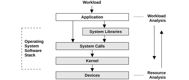
Figure 1.2 Analysis perspectives
The resource analysis perspective is commonly employed by system administrators, who are responsible for the system resources. Application developers, who are responsible for the delivered performance of the workload, commonly focus on the workload analysis perspective. Each perspective has its own strengths, discussed in detail in Chapter 2, Methodologies. For challenging issues, it helps to try analyzing from both perspectives.
1.5 Performance Is Challenging
Systems performance engineering is a challenging field for a number of reasons, including that it is subjective, it is complex, there may not be a single root cause, and it often involves multiple issues.
1.5.1 Subjectivity
Technology disciplines tend to be objective, so much so that people in the industry are known for seeing things in black and white. This can be true of software troubleshooting, where a bug is either present or absent and is either fixed or not fixed. Such bugs often manifest as error messages that can be easily interpreted and understood to mean the presence of an error.
Performance, on the other hand, is often subjective. With performance issues, it can be unclear whether there is an issue to begin with, and if so, when it has been fixed. What may be considered “bad” performance for one user, and therefore an issue, may be considered “good” performance for another.
Consider the following information:
The average disk I/O response time is 1 ms.
Is this “good” or “bad”? While response time, or latency, is one of the best metrics available, interpreting latency information is difficult. To some degree, whether a given metric is “good” or “bad” may depend on the performance expectations of the application developers and end users.
Subjective performance can be made objective by defining clear goals, such as having a target average response time, or requiring a percentage of requests to fall within a certain latency range. Other ways to deal with this subjectivity are introduced in Chapter 2, Methodologies, including latency analysis.
1.5.2 Complexity
In addition to subjectivity, performance can be a challenging discipline due to the complexity of systems and the lack of an obvious starting point for analysis. In cloud computing environments you may not even know which server instance to look at first. Sometimes we begin with a hypothesis, such as blaming the network or a database, and the performance analyst must figure out if this is the right direction.
Performance issues may also originate from complex interactions between subsystems that perform well when analyzed in isolation. This can occur due to a cascading failure, when one failed component causes performance issues in others. To understand the resulting issue, you must untangle the relationships between components and understand how they contribute.
Bottlenecks can also be complex and related in unexpected ways; fixing one may simply move the bottleneck elsewhere in the system, with overall performance not improving as much as hoped.
Apart from the complexity of the system, performance issues may also be caused by a complex characteristic of the production workload. These cases may never be reproducible in a lab environment, or only intermittently so.
Solving complex performance issues often requires a holistic approach. The whole system—both its internals and its external interactions—may need to be investigated. This requires a wide range of skills, and can make performance engineering a varied and intellectually challenging line of work.
Different methodologies can be used to guide us through these complexities, as introduced in Chapter 2; Chapters 6 to 10 include specific methodologies for specific system resources: CPUs, Memory, File Systems, Disks, and Network. (The analysis of complex systems in general, including oil spills and the collapse of financial systems, has been studied by [Dekker 18].)
In some cases, a performance issue can be caused by the interaction of these resources.
1.5.3 Multiple Causes
Some performance issues do not have a single root cause, but instead have multiple contributing factors. Imagine a scenario where three normal events occur simultaneously and combine to cause a performance issue: each is a normal event that in isolation is not the root cause.
Apart from multiple causes, there can also be multiple performance issues.
1.5.4 Multiple Performance Issues
Finding a performance issue is usually not the problem; in complex software there are often many. To illustrate this, try finding the bug database for your operating system or applications and search for the word performance. You might be surprised! Typically, there will be a number of performance issues that are known but not yet fixed, even in mature software that is considered to have high performance. This poses yet another difficulty when analyzing performance: the real task isn’t finding an issue; it’s identifying which issue or issues matter the most.
To do this, the performance analyst must quantify the magnitude of issues. Some performance issues may not apply to your workload, or may apply only to a very small degree. Ideally, you will not just quantify the issues but also estimate the potential speedup to be gained for each one. This information can be valuable when management looks for justification for spending engineering or operations resources.
A metric well suited to performance quantification, when available, is latency.
1.6 Latency
Latency is a measure of time spent waiting, and is an essential performance metric. Used broadly, it can mean the time for any operation to complete, such as an application request, a database query, a file system operation, and so forth. For example, latency can express the time for a website to load completely, from link click to screen paint. This is an important metric for both the customer and the website provider: high latency can cause frustration, and customers may take their business elsewhere.
As a metric, latency can allow maximum speedup to be estimated. For example, Figure 1.3 depicts a database query that takes 100 ms (which is the latency) during which it spends 80 ms blocked waiting for disk reads. The maximum performance improvement by eliminating disk reads (e.g., by caching) can be calculated: from 100 ms to 20 ms (100 – 80) is five times (5x) faster. This is the estimated speedup, and the calculation has also quantified the performance issue: disk reads are causing the query to run up to 5x more slowly.

Figure 1.3 Disk I/O latency example
Such a calculation is not possible when using other metrics. I/O operations per second (IOPS), for example, depend on the type of I/O and are often not directly comparable. If a change were to reduce the IOPS rate by 80%, it is difficult to know what the performance impact would be. There might be 5x fewer IOPS, but what if each of these I/O increased in size (bytes) by 10x?
Latency can also be ambiguous without qualifying terms. For example, in networking, latency can mean the time for a connection to be established but not the data transfer time; or it can mean the total duration of a connection, including the data transfer (e.g., DNS latency is commonly measured this way). Throughout this book I will use clarifying terms where possible: those examples would be better described as connection latency and request latency. Latency terminology is also summarized at the beginning of each chapter.
While latency is a useful metric, it hasn’t always been available when and where needed. Some system areas provide average latency only; some provide no latency measurements at all. With the availability of new BPF2-based observability tools, latency can now be measured from custom arbitrary points of interest and can provide data showing the full distribution of latency.
2BPF is now a name and no longer an acronym (originally Berkeley Packet Filter).
1.7 Observability
Observability refers to understanding a system through observation, and classifies the tools that accomplish this. This includes tools that use counters, profiling, and tracing. It does not include benchmark tools, which modify the state of the system by performing a workload experiment. For production environments, observability tools should be tried first wherever possible, as experimental tools may perturb production workloads through resource contention. For test environments that are idle, you may wish to begin with benchmarking tools to determine hardware performance.
In this section I’ll introduce counters, metrics, profiling, and tracing. I’ll explain observability in more detail in Chapter 4, covering system-wide versus per-process observability, Linux observability tools, and their internals. Chapters 5 to 11 include chapter-specific sections on observability, for example, Section 6.6 for CPU observability tools.
1.7.1 Counters, Statistics, and Metrics
Applications and the kernel typically provide data on their state and activity: operation counts, byte counts, latency measurements, resource utilization, and error rates. They are typically implemented as integer variables called counters that are hard-coded in the software, some of which are cumulative and always increment. These cumulative counters can be read at different times by performance tools for calculating statistics: the rate of change over time, the average, percentiles, etc.
For example, the vmstat(8) utility prints a system-wide summary of virtual memory statistics and more, based on kernel counters in the /proc file system. This example vmstat(8) output is from a 48-CPU production API server:
$ vmstat 1 5
procs -----------memory---------- ---swap-- -----io---- -system-- ------cpu-----
 r  b   swpd   free   buff  cache   si   so    bi    bo   in   cs us sy id wa st
19  0      0 6531592  42656 1672040    0    0     1     7   21   33 51  4 46  0  0
26  0      0 6533412  42656 1672064    0    0     0     0 81262 188942 54  4 43  0  0
62  0      0 6533856  42656 1672088    0    0     0     8 80865 180514 53  4 43  0  0
34  0      0 6532972  42656 1672088    0    0     0     0 81250 180651 53  4 43  0  0
31  0      0 6534876  42656 1672088    0    0     0     0 74389 168210 46  3 51  0  0
This shows a system-wide CPU utilization of around 57% (cpu us + sy columns). The columns are explained in detail in Chapters 6 and 7.
A metric is a statistic that has been selected to evaluate or monitor a target. Most companies use monitoring agents to record selected statistics (metrics) at regular intervals, and chart them in a graphical interface to see changes over time. Monitoring software can also support creating custom alerts from these metrics, such as sending emails to notify staff when problems are detected.
This hierarchy from counters to alerts is depicted in Figure 1.4. Figure 1.4 is provided as a guide to help you understand these terms, but their use in the industry is not rigid. The terms counters, statistics, and metrics are often used interchangeably. Also, alerts may be generated by any layer, and not just a dedicated alerting system.

Figure 1.4 Performance instrumentation terminology
As an example of graphing metrics, Figure 1.5 is a screenshot of a Grafana-based tool observing the same server as the earlier vmstat(8) output.
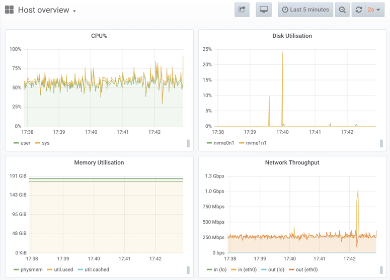
Figure 1.5 System metrics GUI (Grafana)
These line graphs are useful for capacity planning, helping you predict when resources will become exhausted.
Your interpretation of performance statistics will improve with an understanding of how they are calculated. Statistics, including averages, distributions, modes, and outliers, are summarized in Chapter 2, Methodologies, Section 2.8, Statistics.
Sometimes, time-series metrics are all that is needed to resolve a performance issue. Knowing the exact time a problem began may correlate with a known software or configuration change, which can be reverted. Other times, metrics only point in a direction, suggesting that there is a CPU or disk issue, but without explaining why. Profiling or tracing tools are necessary to dig deeper and find the cause.
1.7.2 Profiling
In systems performance, the term profiling usually refers to the use of tools that perform sampling: taking a subset (a sample) of measurements to paint a coarse picture of the target. CPUs are a common profiling target. The commonly used method to profile CPUs involves taking timed-interval samples of the on-CPU code paths.
An effective visualization of CPU profiles is flame graphs. CPU flame graphs can help you find more performance wins than any other tool, after metrics. They reveal not only CPU issues, but other types of issues as well, found by the CPU footprints they leave behind. Issues of lock contention can be found by looking for CPU time in spin paths; memory issues can be analyzed by finding excessive CPU time in memory allocation functions (malloc()), along with the code paths that led to them; performance issues involving misconfigured networking may be discovered by seeing CPU time in slow or legacy codepaths; and so on.
Figure 1.6 is an example CPU flame graph showing the CPU cycles spent by the iperf(1) network micro-benchmark tool.
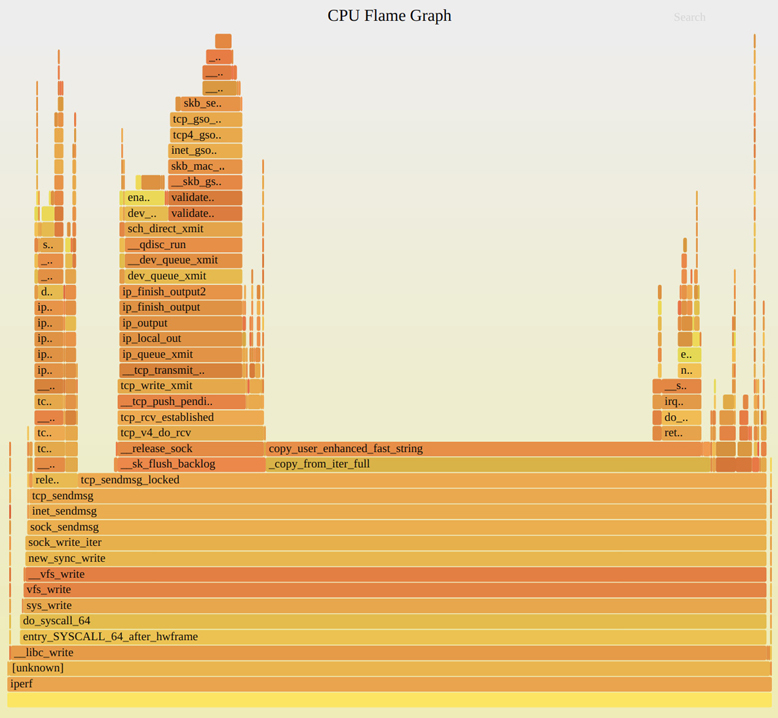
Figure 1.6 CPU profiling using flame graphs
This flame graph shows how much CPU time is spent copying bytes (the path that ends in copy_user_enhanced_fast_string()) versus TCP transmission (the tower on the left that includes tcp_write_xmit()). The widths are proportional to the CPU time spent, and the vertical axis shows the code path.
Profilers are explained in Chapters 4, 5, and 6, and the flame graph visualization is explained in Chapter 6, CPUs, Section 6.7.3, Flame Graphs.
1.7.3 Tracing
Tracing is event-based recording, where event data is captured and saved for later analysis or consumed on-the-fly for custom summaries and other actions. There are special-purpose tracing tools for system calls (e.g., Linux strace(1)) and network packets (e.g., Linux tcpdump(8)); and general-purpose tracing tools that can analyze the execution of all software and hardware events (e.g., Linux Ftrace, BCC, and bpftrace). These all-seeing tracers use a variety of event sources, in particular, static and dynamic instrumentation, and BPF for programmability.
Static Instrumentation
Static instrumentation describes hard-coded software instrumentation points added to the source code. There are hundreds of these points in the Linux kernel that instrument disk I/O, scheduler events, system calls, and more. The Linux technology for kernel static instrumentation is called tracepoints. There is also a static instrumentation technology for user-space software called user statically defined tracing (USDT). USDT is used by libraries (e.g., libc) for instrumenting library calls and by many applications for instrumenting service requests.
As an example tool that uses static instrumentation, execsnoop(8) prints new processes created while it is tracing (running) by instrumenting a tracepoint for the execve(2) system call. The following shows execsnoop(8) tracing an SSH login:
# execsnoop PCOMM PID PPID RET ARGS ssh 30656 20063 0 /usr/bin/ssh 0 sshd 30657 1401 0 /usr/sbin/sshd -D -R sh 30660 30657 0 env 30661 30660 0 /usr/bin/env -i PATH=/usr/local/sbin:/usr/local... run-parts 30661 30660 0 /bin/run-parts --lsbsysinit /etc/update-motd.d 00-header 30662 30661 0 /etc/update-motd.d/00-header uname 30663 30662 0 /bin/uname -o uname 30664 30662 0 /bin/uname -r uname 30665 30662 0 /bin/uname -m 10-help-text 30666 30661 0 /etc/update-motd.d/10-help-text 50-motd-news 30667 30661 0 /etc/update-motd.d/50-motd-news cat 30668 30667 0 /bin/cat /var/cache/motd-news cut 30671 30667 0 /usr/bin/cut -c -80 tr 30670 30667 0 /usr/bin/tr -d �00-�11�13�14�16-�37 head 30669 30667 0 /usr/bin/head -n 10 80-esm 30672 30661 0 /etc/update-motd.d/80-esm lsb_release 30673 30672 0 /usr/bin/lsb_release -cs [...]
This is especially useful for revealing short-lived processes that may be missed by other observability tools such as top(1). These short-lived processes can be a source of performance issues.
See Chapter 4 for more information about tracepoints and USDT probes.
Dynamic Instrumentation
Dynamic instrumentation creates instrumentation points after the software is running, by modifying in-memory instructions to insert instrumentation routines. This is similar to how debuggers can insert a breakpoint on any function in running software. Debuggers pass execution flow to an interactive debugger when the breakpoint is hit, whereas dynamic instrumentation runs a routine and then continues the target software. This capability allows custom performance statistics to be created from any running software. Issues that were previously impossible or prohibitively difficult to solve due to a lack of observability can now be fixed.
Dynamic instrumentation is so different from traditional observation that it can be difficult, at first, to grasp its role. Consider an operating system kernel: analyzing kernel internals can be like venturing into a dark room, with candles (system counters) placed where the kernel engineers thought they were needed. Dynamic instrumentation is like having a flashlight that you can point anywhere.
Dynamic instrumentation was first created in the 1990s [Hollingsworth 94], along with tools that use it called dynamic tracers (e.g., kerninst [Tamches 99]). For Linux, dynamic instrumentation was first developed in 2000 [Kleen 08] and began merging into the kernel in 2004 (kprobes). However, these technologies were not well known and were difficult to use. This changed when Sun Microsystems launched their own version in 2005, DTrace, which was easy to use and production-safe. I developed many DTrace-based tools that showed how important it was for systems performance, tools that saw widespread use and helped make DTrace and dynamic instrumentation well-known.
BPF
BPF, which originally stood for Berkeley Packet Filter, is powering the latest dynamic tracing tools for Linux. BPF originated as a mini in-kernel virtual machine for speeding up the execution of tcpdump(8) expressions. Since 2013 it has been extended (hence is sometimes called eBPF3) to become a generic in-kernel execution environment, one that provides safety and fast access to resources. Among its many new uses are tracing tools, where it provides programmability for the BPF Compiler Collection (BCC) and bpftrace front ends. execsnoop(8), shown earlier, is a BCC tool.4
3eBPF was initially used to describe this extended BPF; however, the technology is now referred to as just BPF.
4I first developed it for DTrace, and I have since developed it for other tracers including BCC and bpftrace.
Chapter 3 explains BPF, and Chapter 15 introduces the BPF tracing front ends: BCC and bpftrace. Other chapters introduce many BPF-based tracing tools in their observability sections; for example, CPU tracing tools are included in Chapter 6, CPUs, Section 6.6, Observability Tools. I have also published prior books on tracing tools (for DTrace [Gregg 11a] and BPF [Gregg 19]).
Both perf(1) and Ftrace are also tracers with some similar capabilities to the BPF front ends. perf(1) and Ftrace are covered in Chapters 13 and 14.
1.8 Experimentation
Apart from observability tools there are also experimentation tools, most of which are benchmarking tools. These perform an experiment by applying a synthetic workload to the system and measuring its performance. This must be done carefully, because experimental tools can perturb the performance of systems under test.
There are macro-benchmark tools that simulate a real-world workload such as clients making application requests; and there are micro-benchmark tools that test a specific component, such as CPUs, disks, or networks. As an analogy: a car’s lap time at Laguna Seca Raceway could be considered a macro-benchmark, whereas its top speed and 0 to 60mph time could be considered micro-benchmarks. Both benchmark types are important, although micro-benchmarks are typically easier to debug, repeat, and understand, and are more stable.
The following example uses iperf(1) on an idle server to perform a TCP network throughput micro-benchmark with a remote idle server. This benchmark ran for ten seconds (-t 10) and produces per-second averages (-i 1):
# iperf -c 100.65.33.90 -i 1 -t 10
------------------------------------------------------------
Client connecting to 100.65.33.90, TCP port 5001
TCP window size: 12.0 MByte (default)
------------------------------------------------------------
[  3] local 100.65.170.28 port 39570 connected with 100.65.33.90 port 5001
[ ID] Interval       Transfer     Bandwidth
[  3]  0.0- 1.0 sec   582 MBytes  4.88 Gbits/sec
[  3]  1.0- 2.0 sec   568 MBytes  4.77 Gbits/sec
[  3]  2.0- 3.0 sec   574 MBytes  4.82 Gbits/sec
[  3]  3.0- 4.0 sec   571 MBytes  4.79 Gbits/sec
[  3]  4.0- 5.0 sec   571 MBytes  4.79 Gbits/sec
[  3]  5.0- 6.0 sec   432 MBytes  3.63 Gbits/sec
[  3]  6.0- 7.0 sec   383 MBytes  3.21 Gbits/sec
[  3]  7.0- 8.0 sec   388 MBytes  3.26 Gbits/sec
[  3]  8.0- 9.0 sec   390 MBytes  3.28 Gbits/sec
[  3]  9.0-10.0 sec   383 MBytes  3.22 Gbits/sec
[  3]  0.0-10.0 sec  4.73 GBytes  4.06 Gbits/sec
The output shows a throughput5 of around 4.8 Gbits for the first five seconds, which drops to around 3.2 Gbits/sec. This is an interesting result that shows bi-modal throughput. To improve performance, one might focus on the 3.2 Gbits/sec mode, and search for other metrics that can explain it.
5The output uses the term “Bandwidth,” a common misuse. Bandwidth refers to the maximum possible throughput, which iperf(1) is not measuring. iperf(1) is measuring the current rate of its network workload: its throughput.
Consider the drawbacks of debugging this performance issue on a production server using observability tools alone. Network throughput can vary from second to second because of natural variance in the client workload, and the underlying bi-modal behavior of the network might not be apparent. By using iperf(1) with a fixed workload, you eliminate client variance, revealing the variance due to other factors (e.g., external network throttling, buffer utilization, and so on).
As I recommended earlier, on production systems you should first try observability tools. However, there are so many observability tools that you might spend hours working through them when an experimental tool would lead to quicker results. An analogy taught to me by a senior performance engineer (Roch Bourbonnais) many years ago was this: you have two hands, observability and experimentation. Only using one type of tool is like trying to solve a problem one-handed.
Chapters 6 to 10 include sections on experimental tools; for example, CPU experimental tools are covered in Chapter 6, CPUs, Section 6.8, Experimentation.
1.9 Cloud Computing
Cloud computing, a way to deploy computing resources on demand, has enabled rapid scaling of applications by supporting their deployment across an increasing number of small virtual systems called instances. This has decreased the need for rigorous capacity planning, as more capacity can be added from the cloud at short notice. In some cases it has also increased the desire for performance analysis, because using fewer resources can mean fewer systems. Since cloud usage is typically charged by the minute or hour, a performance win resulting in fewer systems can mean immediate cost savings. Compare this scenario to an enterprise data center, where you may be locked into a fixed support contract for years, unable to realize cost savings until the contract has ended.
New difficulties caused by cloud computing and virtualization include the management of performance effects from other tenants (sometimes called performance isolation) and physical system observability from each tenant. For example, unless managed properly by the system, disk I/O performance may be poor due to contention with a neighbor. In some environments, the true usage of the physical disks may not be observable by each tenant, making identification of this issue difficult.
These topics are covered in Chapter 11, Cloud Computing.
1.10 Methodologies
Methodologies are a way to document the recommended steps for performing various tasks in systems performance. Without a methodology, a performance investigation can turn into a fishing expedition: trying random things in the hope of catching a win. This can be time-consuming and ineffective, while allowing important areas to be overlooked. Chapter 2, Methodologies, includes a library of methodologies for systems performance. The following is the first I use for any performance issue: a tool-based checklist.
1.10.1 Linux Perf Analysis in 60 Seconds
This is a Linux tool-based checklist that can be executed in the first 60 seconds of a performance issue investigation, using traditional tools that should be available for most Linux distributions [Gregg 15a]. Table 1.1 shows the commands, what to check for, and the section in this book that covers the command in more detail.
Table 1.1 Linux 60-second analysis checklist
# |
Tool |
Check |
Section |
|---|---|---|---|
1 |
|
Load averages to identify if load is increasing or decreasing (compare 1-, 5-, and 15-minute averages). |
|
2 |
|
Kernel errors including OOM events. |
|
3 |
|
System-wide statistics: run queue length, swapping, overall CPU usage. |
|
4 |
|
Per-CPU balance: a single busy CPU can indicate poor thread scaling. |
|
5 |
|
Per-process CPU usage: identify unexpected CPU consumers, and user/system CPU time for each process. |
|
6 |
|
Disk I/O statistics: IOPS and throughput, average wait time, percent busy. |
|
7 |
|
Memory usage including the file system cache. |
|
8 |
|
Network device I/O: packets and throughput. |
|
9 |
|
TCP statistics: connection rates, retransmits. |
|
10 |
|
Check overview. |
This checklist can also be followed using a monitoring GUI, provided the same metrics are available.6
6You could even make a custom dashboard for this checklist; however, bear in mind that this checklist was designed to make the most of readily available CLI tools, and monitoring products may have more (and better) metrics available. I’d be more inclined to make custom dashboards for the USE method and other methodologies.
Chapter 2, Methodologies, as well as later chapters, contain many more methodologies for performance analysis, including the USE method, workload characterization, latency analysis, and more.
1.11 Case Studies
If you are new to systems performance, case studies showing when and why various activities are performed can help you relate them to your current environment. Two hypothetical examples are summarized here; one is a performance issue involving disk I/O, and one is performance testing of a software change.
These case studies describe activities that are explained in other chapters of this book. The approaches described here are also intended to show not the right way or the only way, but rather a way that these performance activities can be conducted, for your critical consideration.
1.11.1 Slow Disks
Sumit is a system administrator at a medium-size company. The database team has filed a support ticket complaining of “slow disks” on one of their database servers.
Sumit’s first task is to learn more about the issue, gathering details to form a problem statement. The ticket claims that the disks are slow, but it doesn’t explain whether this is causing a database issue or not. Sumit responds by asking these questions:
Is there currently a database performance issue? How is it measured?
How long has this issue been present?
Has anything changed with the database recently?
Why were the disks suspected?
The database team replies: “We have a log for queries slower than 1,000 milliseconds. These usually don’t happen, but during the past week they have been growing to dozens per hour. AcmeMon showed that the disks were busy.”
This confirms that there is a real database issue, but it also shows that the disk hypothesis is likely a guess. Sumit wants to check the disks, but he also wants to check other resources quickly in case that guess was wrong.
AcmeMon is the company’s basic server monitoring system, providing historical performance graphs based on standard operating system metrics, the same metrics printed by mpstat(1), iostat(1), and system utilities. Sumit logs in to AcmeMon to see for himself.
Sumit begins with a methodology called the USE method (defined in Chapter 2, Methodologies, Section 2.5.9) to quickly check for resource bottlenecks. As the database team reported, utilization for the disks is high, around 80%, while for the other resources (CPU, network) utilization is much lower. The historical data shows that disk utilization has been steadily increasing during the past week, while CPU utilization has been steady. AcmeMon doesn’t provide saturation or error statistics for the disks, so to complete the USE method Sumit must log in to the server and run some commands.
He checks disk error counters from /sys; they are zero. He runs iostat(1) with an interval of one second and watches utilization and saturation metrics over time. AcmeMon reported 80% utilization but uses a one-minute interval. At one-second granularity, Sumit can see that disk utilization fluctuates, often hitting 100% and causing levels of saturation and increased disk I/O latency.
To further confirm that this is blocking the database—and isn’t asynchronous with respect to the database queries—he uses a BCC/BPF tracing tool called offcputime(8) to capture stack traces whenever the database was descheduled by the kernel, along with the time spent off-CPU. The stack traces show that the database is often blocking during a file system read, during a query. This is enough evidence for Sumit.
The next question is why. The disk performance statistics appear to be consistent with high load. Sumit performs workload characterization to understand this further, using iostat(1) to measure IOPS, throughput, average disk I/O latency, and the read/write ratio. For more details, Sumit can use disk I/O tracing; however, he is satisfied that this already points to a case of high disk load, and not a problem with the disks.
Sumit adds more details to the ticket, stating what he checked and including screenshots of the commands used to study the disks. His summary so far is that the disks are under high load, which increases I/O latency and is slowing the queries. However, the disks appear to be acting normally for the load. He asks if there is a simple explanation: did the database load increase?
The database team responds that it did not, and that the rate of queries (which isn’t reported by AcmeMon) has been steady. This sounds consistent with an earlier finding, that CPU utilization was also steady.
Sumit thinks about what else could cause higher disk I/O load without a noticeable increase in CPU and has a quick talk with his colleagues about it. One of them suggests file system fragmentation, which is expected when the file system approaches 100% capacity. Sumit finds that it is only at 30%.
Sumit knows he can perform drill-down analysis7 to understand the exact causes of disk I/O, but this can be time-consuming. He tries to think of other easy explanations that he can check quickly first, based on his knowledge of the kernel I/O stack. He remembers that this disk I/O is largely caused by file system cache (page cache) misses.
7This is covered in Chapter 2, Methodologies, Section 2.5.12, Drill-Down Analysis.
Sumit checks the file system cache hit ratio using cachestat(8)8 and finds it is currently at 91%. This sounds high (good), but he has no historical data to compare it to. He logs in to other database servers that serve similar workloads and finds their cache hit ratio to be over 98%. He also finds that the file system cache size is much larger on the other servers.
8A BCC tracing tool covered in Chapter 8, File Systems, Section 8.6.12, cachestat.
Turning his attention to the file system cache size and server memory usage, he finds something that had been overlooked: a development project has a prototype application that is consuming a growing amount of memory, even though it isn’t under production load yet. This memory is taken from what is available for the file system cache, reducing its hit rate and causing more file system reads to become disk reads.
Sumit contacts the application development team and asks them to shut down the application and move it to a different server, referring to the database issue. After they do this, Sumit watches disk utilization creep downward in AcmeMon as the file system cache recovers to its original size. The slow queries return to zero, and he closes the ticket as resolved.
1.11.2 Software Change
Pamela is a performance and scalability engineer at a small company where she works on all performance-related activities. The application developers have developed a new core feature and are unsure whether its introduction could hurt performance. Pamela decides to perform non-regression testing9 of the new application version, before it is deployed in production.
9Some call it regression testing, but it is an activity intended to confirm that a software or hardware change does not cause performance to regress, hence, non-regression testing.
Pamela acquires an idle server for the purpose of testing and searches for a client workload simulator. The application team had written one a while ago, although it has various limitations and known bugs. She decides to try it but wants to confirm that it adequately resembles the current production workload.
She configures the server to match the current deployment configuration and runs the client workload simulator from a different system to the server. The client workload can be characterized by studying an access log, and there is already a company tool to do this, which she uses. She also runs the tool on a production server log for different times of day and compares workloads. It appears that the client simulator applies an average production workload but doesn’t account for variance. She notes this and continues her analysis.
Pamela knows a number of approaches to use at this point. She picks the easiest: increasing load from the client simulator until a limit is reached (this is sometimes called stress testing). The client simulator can be configured to execute a target number of client requests per second, with a default of 1,000 that she had used earlier. She decides to increase load starting at 100 and adding increments of 100 until a limit is reached, each level being tested for one minute. She writes a shell script to perform the test, which collects results in a file for plotting by other tools.
With the load running, she performs active benchmarking to determine what the limiting factors are. The server resources and server threads seem largely idle. The client simulator shows that the request throughput levels off at around 700 per second.
She switches to the new software version and repeats the test. This also reaches the 700 mark and levels off. She also analyzes the server to look for limiting factors but again cannot see any.
She plots the results, showing completed request rate versus load, to visually identify the scalability profile. Both appear to reach an abrupt ceiling.
While it appears that the software versions have similar performance characteristics, Pamela is disappointed that she wasn’t able to identify the limiting factor causing the scalability ceiling. She knows she checked only server resources, and the limiter could instead be an application logic issue. It could also be elsewhere: the network or the client simulator.
Pamela wonders if a different approach may be needed, such as running a fixed rate of operations and then characterizing resource usage (CPU, disk I/O, network I/O), so that it can be expressed in terms of a single client request. She runs the simulator at a rate of 700 per second for the current and new software and measures resource consumption. The current software drove the 32 CPUs to an average of 20% utilization for the given load. The new software drove the same CPUs to 30% utilization, for the same load. It would appear that this is indeed a regression, one that consumes more CPU resources.
Curious to understand the 700 limit, Pamela launches a higher load and then investigates all components in the data path, including the network, the client system, and the client workload generator. She also performs drill-down analysis of the server and client software. She documents what she has checked, including screenshots, for reference.
To investigate the client software she performs thread state analysis and finds that it is single-threaded! That one thread is spending 100% of its time executing on-CPU. This convinces her that this is the limiter of the test.
As an experiment, she launches the client software in parallel on different client systems. In this way, she drives the server to 100% CPU utilization for both the current and new software. The current version reaches 3,500 requests/sec, and the new version 2,300 requests/sec, consistent with earlier findings of resource consumption.
Pamela informs the application developers that there is a regression with the new software version, and she begins to profile its CPU usage using a CPU flame graph to understand why: what code paths are contributing. She notes that an average production workload was tested and that varied workloads were not. She also files a bug to note that the client workload generator is single-threaded, which can become a bottleneck.
1.11.3 More Reading
A more detailed case study is provided as Chapter 16, Case Study, which documents how I resolved a particular cloud performance issue. The next chapter introduces the methodologies used for performance analysis, and the remaining chapters cover the necessary background and specifics.
1.12 References
[Hollingsworth 94] Hollingsworth, J., Miller, B., and Cargille, J., “Dynamic Program Instrumentation for Scalable Performance Tools,” Scalable High-Performance Computing Conference (SHPCC), May 1994.
[Tamches 99] Tamches, A., and Miller, B., “Fine-Grained Dynamic Instrumentation of Commodity Operating System Kernels,” Proceedings of the 3rd Symposium on Operating Systems Design and Implementation, February 1999.
[Kleen 08] Kleen, A., “On Submitting Kernel Patches,” Intel Open Source Technology Center, http://halobates.de/on-submitting-patches.pdf, 2008.
[Gregg 11a] Gregg, B., and Mauro, J., DTrace: Dynamic Tracing in Oracle Solaris, Mac OS X and FreeBSD, Prentice Hall, 2011.
[Gregg 15a] Gregg, B., “Linux Performance Analysis in 60,000 Milliseconds,” Netflix Technology Blog, http://techblog.netflix.com/2015/11/linux-performance-analysis-in-60s.html, 2015.
[Dekker 18] Dekker, S., Drift into Failure: From Hunting Broken Components to Understanding Complex Systems, CRC Press, 2018.
[Gregg 19] Gregg, B., BPF Performance Tools: Linux System and Application Observability, Addison-Wesley, 2019.
[Corry 20] Corry, A., Retrospectives Antipatterns, Addison-Wesley, 2020.