CHAPTER 4
Row-Pattern Recognition in SQL
This book is dedicated to using window functions in your T-SQL code. In large part, the book covers windowing and related analytical features that at the date of this writing have already been implemented in T-SQL. That’s what you would naturally expect from a book entitled “T-SQL Window Functions.” However, as you’ve already noticed, the book also exposes you to features that are part of the SQL standard but that have not yet been implemented in T-SQL. I find this coverage just as important. It raises awareness to what’s out there, and hopefully, it will motivate you, as part of the Microsoft data platform community, to ask Microsoft to improve SQL Server and Azure SQL Database by adding such features to T-SQL. In fact, quite a few of the existing windowing features in T-SQL were added as a result of past community efforts. Microsoft is listening!
Previous chapters had mixed coverage, including both features that have already been implemented in T-SQL and of related features from the SQL standard that were not. This chapter’s focus is an immensely powerful concept from the SQL standard called row-pattern recognition, which involves a number of features—none of which are available in T-SQL yet. Understanding that your time is valuable and that you may prefer to focus only on functionality that is already available in T-SQL, I wanted to give you a heads up so that you can elect to skip this chapter. However, if you do wish to know what is part of modern SQL but is not yet available in T-SQL, you will probably want to carry on reading this chapter.

Note Once you’re done, you can help improve T-SQL by casting your vote on the suggestion to “Add Support for Row-Pattern Recognition in T-SQL (SQL:2016 features R010 and R020),” which can be found at https://feedback.azure.com/forums/908035-sqlserver/suggestions/37251232-add-support-for-row-pattern-recognition-in-t-sql.
Background
Row-pattern recognition, or RPR in short, enables you to use regular expressions to identify patterns in sequences of rows similar to the way you use regular expressions to identify patterns in character strings. You could be looking for certain patterns in stock market trading activity, time series, shipping data, material handling, DNA sequences, temperature measurements, gas emissions, and other sequences of rows. Those patterns could be meaningful to you, enabling you to derive valuable trading information, detect potentially fraudulent activity, identify trends, find gaps and islands in your data, and more. RPR uses an elegant design that makes it easy to define the patterns that you’re looking for and to act on the matches with all sorts of computations.
To me, RPR is the next step in the evolution of window functions into a more sophisticated and highly flexible analytical tool. Similar to window functions, RPR uses partitioning and ordering. Row-pattern partitioning allows you to act on each partition of rows independently, and row-pattern ordering defines the order to be used for finding pattern matches in the partition. Additional elements in the RPR specification allow you to use regular expressions to define the pattern that you’re looking for, and they allow you to apply computations against the matches. You can then elect to either
■ Return one summary row per match, similar to grouping
■ Return all rows per match, which gives you the detail rows
Note The ISO/IEC SQL 9075:2016 standard, or SQL:2016 in short, has extensive coverage of row-pattern recognition and features that use the concept. You can find the coverage in two main documents. One document is “ISO/IEC 9075-2:2016, Information technology— Database languages—SQL—Part 2: Foundation (SQL/Foundation),” which is the document containing the SQL standard’s core language elements. It covers row-pattern recognition among many of the other core SQL features. This document is available for purchase at https://www.iso.org/standard/63556.html. Another document is a 90-page technical review called “ISO/IEC TR 19075-5,” which is dedicated specifically to row-pattern recognition. This document is available for free at https://standards.iso.org/ittf/PubliclyAvailableStandards/c065143_ISO_IEC_TR_19075-5_2016.zip.
The SQL standard defines two main features that use row-pattern recognition:
■ Feature R010, “Row-pattern recognition: FROM clause”
■ Feature R020, “Row-pattern recognition: WINDOW clause”
With feature R010, you use row-pattern recognition in a table operator called MATCH_RECOGNIZE within the FROM clause. With feature R020, you use row-pattern recognition in a window specification to restrict the full window frame into a reduced window frame that is based on a pattern match. The standard also briefly mentions feature R030, “Row-pattern recognition: full aggregate support,” without which an aggregate function used in row-pattern recognition shall not specify DISTINCT or <filter clause>.
This chapter covers row-pattern recognition in three main sections. The first covers feature R010, the second covers feature R020, and the third covers solutions using row-pattern recognition.
Note Oracle is an example for a database platform that implements feature R010 (introduced in version 12c). I do not know of any platform that implements feature R020 yet. Therefore, I was able to test solutions related to feature R010 on Oracle, but I could not test the solutions related to R020. In case you have access to Oracle (it’s a free download for testing purposes) and wish to run the solutions from the section on feature R010, by all means, I encourage you to do so. Language features are so much better understood if you can experiment with code that uses them. Therefore, I’ll provide both theoretical T-SQL code that is not runnable at the date of this writing—as well as Oracle code that is actually runnable today—or instructions for how to adapt the T-SQL code to be runnable on Oracle.
Feature R010, “Row-Pattern Recognition: FROM Clause”
Feature R010, “Row-pattern recognition: FROM clause,” defines a table operator called MATCH_ RECOGNIZE, which you use in the FROM clause much like you use the JOIN, APPLY, PIVOT, and UNPIVOT operators. The input is a table or table expression, and the output is a virtual table. Here’s the general form of a query using the MATCH_RECOGNIZE operator:
SELECT <select list>
FROM <source table>
  MATCH_RECOGNIZE
  (
    [ PARTITION BY <partition list> ]
    [ ORDER BY <order by list> ]
    [ MEASURES <measure list> ]
    [ <row-pattern rows per match> ::=
        ONE ROW PER MATCH | ALL ROWS PER MATCH ]
    [ AFTER MATCH <skip to option>
    PATTERN ( <row-pattern> )
    [ SUBSET <subset list> ]
    DEFINE <definition list>
  ) AS <table alias>;
From a logical query processing standpoint, much like the other table operators, the MATCH_RECOGNIZE operator is processed as a step within the FROM clause. It can operate directly on an input table or table expression, or it can operate on a virtual table resulting from other table operators. Similarly, its output virtual table can be used as an input to another table operator.
The following sections describe the MATCH_RECOGNIZE operator and its options, illustrated through a sample task.
Sample Task
I’ll illustrate the use of the MATCH_RECOGNIZE operator through a sample task adapted from the aforementioned technical review (called “ISO/IEC TR 19075-5”). For this purpose, I’ll use a table called Ticker, with columns symbol, tradedate, and price, holding daily closing trading prices for a couple of stock ticker symbols.
Use the code in Listing 4-1 to create and populate the dbo.Ticker table in SQL Server in the sample database TSQLV5.
LISTING 4-1 Sample Data in Microsoft SQL Server
SET NOCOUNT ON;
USE TSQLV5;

DROP TABLE IF EXISTS dbo.Ticker;

CREATE TABLE dbo.Ticker
(
  symbol    VARCHAR(10)    NOT NULL,
  tradedate DATE           NOT NULL,
  price     NUMERIC(12, 2) NOT NULL,
  CONSTRAINT PK_Ticker
    PRIMARY KEY (symbol, tradedate)
);
GO

INSERT INTO dbo.Ticker(symbol, tradedate, price) VALUES
  ('STOCK1', '20190212', 150.00),
  ('STOCK1', '20190213', 151.00),
  ('STOCK1', '20190214', 148.00),
  ('STOCK1', '20190215', 146.00),
  ('STOCK1', '20190218', 142.00),
  ('STOCK1', '20190219', 144.00),
  ('STOCK1', '20190220', 152.00),
  ('STOCK1', '20190221', 152.00),
  ('STOCK1', '20190222', 153.00),
  ('STOCK1', '20190225', 154.00),
  ('STOCK1', '20190226', 154.00),
  ('STOCK1', '20190227', 154.00),
  ('STOCK1', '20190228', 153.00),
  ('STOCK1', '20190301', 145.00),
  ('STOCK1', '20190304', 140.00),
  ('STOCK1', '20190305', 142.00),
  ('STOCK1', '20190306', 143.00),
  ('STOCK1', '20190307', 142.00),
  ('STOCK1', '20190308', 140.00),
  ('STOCK1', '20190311', 138.00),
  ('STOCK2', '20190212', 330.00),
  ('STOCK2', '20190213', 329.00),
  ('STOCK2', '20190214', 329.00),
  ('STOCK2', '20190215', 326.00),
  ('STOCK2', '20190218', 325.00),
  ('STOCK2', '20190219', 326.00),
  ('STOCK2', '20190220', 328.00),
  ('STOCK2', '20190221', 326.00),
  ('STOCK2', '20190222', 320.00),
  ('STOCK2', '20190225', 317.00),
  ('STOCK2', '20190226', 319.00),
  ('STOCK2', '20190227', 325.00),
  ('STOCK2', '20190228', 322.00),
  ('STOCK2', '20190301', 324.00),
  ('STOCK2', '20190304', 321.00),
  ('STOCK2', '20190305', 319.00),
  ('STOCK2', '20190306', 322.00),
  ('STOCK2', '20190307', 326.00),
  ('STOCK2', '20190308', 326.00),
  ('STOCK2', '20190311', 324.00);

SELECT symbol, tradedate, price
FROM dbo.Ticker;
The last query shows the contents of the table, generating the output shown in Listing 4-2.
LISTING 4-2 Contents of dbo. Ticker Table
symbol  tradedate   price
------- ----------- -------
STOCK1  2019-02-12  150.00
STOCK1  2019-02-13  151.00
STOCK1  2019-02-14  148.00
STOCK1  2019-02-15  146.00
STOCK1  2019-02-18  142.00
STOCK1  2019-02-19  144.00
STOCK1  2019-02-20  152.00
STOCK1  2019-02-21  152.00
STOCK1  2019-02-22  153.00
STOCK1  2019-02-25  154.00
STOCK1  2019-02-26  154.00
STOCK1  2019-02-27  154.00
STOCK1  2019-02-28  153.00
STOCK1  2019-03-01  145.00
STOCK1  2019-03-04  140.00
STOCK1  2019-03-05  142.00
STOCK1  2019-03-06  143.00
STOCK1  2019-03-07  142.00
STOCK1  2019-03-08  140.00
STOCK1  2019-03-11  138.00
STOCK2  2019-02-12  330.00
STOCK2  2019-02-13  329.00
STOCK2  2019-02-14  329.00
STOCK2  2019-02-15  326.00
STOCK2  2019-02-18  325.00
STOCK2  2019-02-19  326.00
STOCK2  2019-02-20  328.00
STOCK2  2019-02-21  326.00
STOCK2  2019-02-22  320.00
STOCK2  2019-02-25  317.00
STOCK2  2019-02-26  319.00
STOCK2  2019-02-27  325.00
STOCK2  2019-02-28  322.00
STOCK2  2019-03-01  324.00
STOCK2  2019-03-04  321.00
STOCK2  2019-03-05  319.00
STOCK2  2019-03-06  322.00
STOCK2  2019-03-07  326.00
STOCK2  2019-03-08  326.00
STOCK2  2019-03-11  324.00
In case you are planning to run the code samples on Oracle, use the code in Listing 4-3 to create and populate the Ticker table there.
LISTING 4-3 Sample Data in Oracle
DROP TABLE Ticker;

CREATE TABLE Ticker
(
  symbol    VARCHAR2(10) NOT NULL,
  tradedate DATE         NOT NULL,
  price     NUMBER       NOT NULL,
  CONSTRAINT PK_Ticker
    PRIMARY KEY (symbol, tradedate)
);

INSERT INTO Ticker(symbol, tradedate, price)
  VALUES('STOCK1', '12-Feb-19', 150.00);
INSERT INTO Ticker(symbol, tradedate, price)
  VALUES('STOCK1', '13-Feb-19', 151.00);
INSERT INTO Ticker(symbol, tradedate, price)
  VALUES('STOCK1', '14-Feb-19', 148.00);
INSERT INTO Ticker(symbol, tradedate, price)
  VALUES('STOCK1', '15-Feb-19', 146.00);
INSERT INTO Ticker(symbol, tradedate, price)
  VALUES('STOCK1', '18-Feb-19', 142.00);
INSERT INTO Ticker(symbol, tradedate, price)
  VALUES('STOCK1', '19-Feb-19', 144.00);
INSERT INTO Ticker(symbol, tradedate, price)
  VALUES('STOCK1', '20-Feb-19', 152.00);
INSERT INTO Ticker(symbol, tradedate, price)
  VALUES('STOCK1', '21-Feb-19', 152.00);
INSERT INTO Ticker(symbol, tradedate, price)
  VALUES('STOCK1', '22-Feb-19', 153.00);
INSERT INTO Ticker(symbol, tradedate, price)
  VALUES('STOCK1', '25-Feb-19', 154.00);
INSERT INTO Ticker(symbol, tradedate, price)
  VALUES('STOCK1', '26-Feb-19', 154.00);
INSERT INTO Ticker(symbol, tradedate, price)
  VALUES('STOCK1', '27-Feb-19', 154.00);
INSERT INTO Ticker(symbol, tradedate, price)
  VALUES('STOCK1', '28-Feb-19', 153.00);
INSERT INTO Ticker(symbol, tradedate, price)
  VALUES('STOCK1', '01-Mar-19', 145.00);
INSERT INTO Ticker(symbol, tradedate, price)
  VALUES('STOCK1', '04-Mar-19', 140.00);
INSERT INTO Ticker(symbol, tradedate, price)
  VALUES('STOCK1', '05-Mar-19', 142.00);
INSERT INTO Ticker(symbol, tradedate, price)
  VALUES('STOCK1', '06-Mar-19', 143.00);
INSERT INTO Ticker(symbol, tradedate, price)
  VALUES('STOCK1', '07-Mar-19', 142.00);
INSERT INTO Ticker(symbol, tradedate, price)
  VALUES('STOCK1', '08-Mar-19', 140.00);
INSERT INTO Ticker(symbol, tradedate, price)
  VALUES('STOCK1', '11-Mar-19', 138.00);
INSERT INTO Ticker(symbol, tradedate, price)
  VALUES('STOCK2', '12-Feb-19', 330.00);
INSERT INTO Ticker(symbol, tradedate, price)
  VALUES('STOCK2', '13-Feb-19', 329.00);
INSERT INTO Ticker(symbol, tradedate, price)
  VALUES('STOCK2', '14-Feb-19', 329.00);
INSERT INTO Ticker(symbol, tradedate, price)
  VALUES('STOCK2', '15-Feb-19', 326.00);
INSERT INTO Ticker(symbol, tradedate, price)
  VALUES('STOCK2', '18-Feb-19', 325.00);
INSERT INTO Ticker(symbol, tradedate, price)
  VALUES('STOCK2', '19-Feb-19', 326.00);
INSERT INTO Ticker(symbol, tradedate, price)
  VALUES('STOCK2', '20-Feb-19', 328.00);
INSERT INTO Ticker(symbol, tradedate, price)
  VALUES('STOCK2', '21-Feb-19', 326.00);
INSERT INTO Ticker(symbol, tradedate, price)
  VALUES('STOCK2', '22-Feb-19', 320.00);
INSERT INTO Ticker(symbol, tradedate, price)
  VALUES('STOCK2', '25-Feb-19', 317.00);
INSERT INTO Ticker(symbol, tradedate, price)
  VALUES('STOCK2', '26-Feb-19', 319.00);
INSERT INTO Ticker(symbol, tradedate, price)
  VALUES('STOCK2', '27-Feb-19', 325.00);
INSERT INTO Ticker(symbol, tradedate, price)
  VALUES('STOCK2', '28-Feb-19', 322.00);
INSERT INTO Ticker(symbol, tradedate, price)
  VALUES('STOCK2', '01-Mar-19', 324.00);
INSERT INTO Ticker(symbol, tradedate, price)
  VALUES('STOCK2', '04-Mar-19', 321.00);
INSERT INTO Ticker(symbol, tradedate, price)
  VALUES('STOCK2', '05-Mar-19', 319.00);
INSERT INTO Ticker(symbol, tradedate, price)
  VALUES('STOCK2', '06-Mar-19', 322.00);
INSERT INTO Ticker(symbol, tradedate, price)
  VALUES('STOCK2', '07-Mar-19', 326.00);
INSERT INTO Ticker(symbol, tradedate, price)
  VALUES('STOCK2', '08-Mar-19', 326.00);
INSERT INTO Ticker(symbol, tradedate, price)
  VALUES('STOCK2', '11-Mar-19', 324.00);
COMMIT;

SELECT symbol, tradedate, price
FROM Ticker;
The query showing the contents of the table generates the output shown in Listing 4-4.
LISTING 4-4 Contents of Ticker Table
SYMBOL     TRADEDATE      PRICE
---------- --------- ----------
STOCK1     12-FEB-19        150
STOCK1     13-FEB-19        151
STOCK1     14-FEB-19        148
STOCK1     15-FEB-19        146
STOCK1     18-FEB-19        142
STOCK1     19-FEB-19        144
STOCK1     20-FEB-19        152
STOCK1     21-FEB-19        152
STOCK1     22-FEB-19        153
STOCK1     25-FEB-19        154
STOCK1     26-FEB-19        154
STOCK1     27-FEB-19        154
STOCK1     28-FEB-19        153
STOCK1     01-MAR-19        145
STOCK1     04-MAR-19        140
STOCK1     05-MAR-19        142
STOCK1     06-MAR-19        143
STOCK1     07-MAR-19        142
STOCK1     08-MAR-19        140
STOCK1     11-MAR-19        138
STOCK2     12-FEB-19        330
STOCK2     13-FEB-19        329
STOCK2     14-FEB-19        329
STOCK2     15-FEB-19        326
STOCK2     18-FEB-19        325
STOCK2     19-FEB-19        326
STOCK2     20-FEB-19        328
STOCK2     21-FEB-19        326
STOCK2     22-FEB-19        320
STOCK2     25-FEB-19        317
STOCK2     26-FEB-19        319
STOCK2     27-FEB-19        325
STOCK2     28-FEB-19        322
STOCK2     01-MAR-19        324
STOCK2     04-MAR-19        321
STOCK2     05-MAR-19        319
STOCK2     06-MAR-19        322
STOCK2     07-MAR-19        326
STOCK2     08-MAR-19        326
STOCK2     11-MAR-19        324
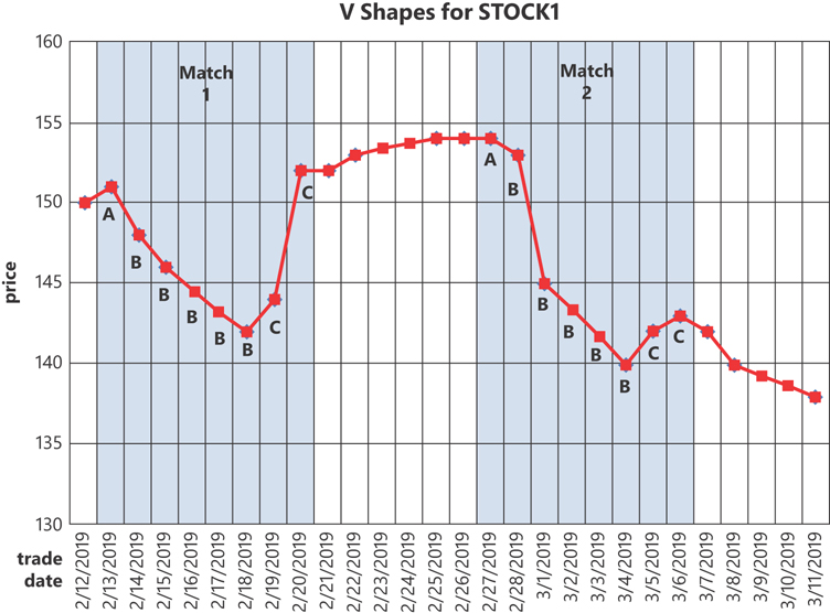
You’re given a task to query the Ticker table and identify sequences of rows representing V shapes in the trading activity, for each symbol independently, based on trading date order. A V shape means a consecutive sequence of rows starting with any row, immediately followed by a period of strictly decreasing prices, immediately followed by a period of strictly increasing prices. We can find these sorts of price change occurrences using row-pattern recognition.
Figure 4-1 shows a visual depiction of the V-shape pattern matches that the solution query finds for STOCK1.
As part of the specification of the MATCH_RECOGNIZE operator, you indicate a row-pattern rows per match option where you indicate whether you want the output table to have one summary row per match, like in grouping, or all rows per match, where you get the detail rows. In the following sections I demonstrate both options.
ONE ROW PER MATCH
Listing 4-5 has the solution query for the sample task, showing one row per match with the summary information, followed by the query’s expected output (split into two parts due to page size restrictions).
LISTING 4-5 Solution Query for Sample Task with the ONE ROW PER MATCH Option
SELECT
  MR.symbol, MR.matchnum, MR.startdate, MR.startprice,
  MR.bottomdate, MR.bottomprice, MR.enddate, MR.endprice, MR.maxprice
FROM dbo.Ticker
  MATCH_RECOGNIZE
  (
    PARTITION BY symbol
    ORDER BY tradedate
    MEASURES
      MATCH_NUMBER() AS matchnum,
      A.tradedate AS startdate,
      A.price AS startprice,
      LAST(B.tradedate) AS bottomdate,
      LAST(B.price) AS bottomprice,
      LAST(C.tradedate) AS enddate, -- same as LAST(tradedate)
      LAST(C.price) AS endprice,
      MAX(U.price) AS maxprice -- same as MAX(price)
    ONE ROW PER MATCH -- default
    AFTER MATCH SKIP PAST LAST ROW -- default
    PATTERN (A B+ C+)
    SUBSET U = (A, B, C)
    DEFINE
      -- A defaults to True, matches any row, same as A AS 1 = 1
      B AS B.price < PREV(B.price),
      C AS C.price > PREV(C.price)
  ) AS MR;

symbol  matchnum  startdate   startprice bottomdate  bottomprice
------- --------- ----------- ---------- ----------- -----------
STOCK1  1         2019-02-13  151.00     2019-02-18  142.00
STOCK1  2         2019-02-27  154.00     2019-03-04  140.00
STOCK2  1         2019-02-14  329.00     2019-02-18  325.00
STOCK2  2         2019-02-21  326.00     2019-02-25  317.00
STOCK2  3         2019-03-01  324.00     2019-03-05  319.00

symbol  matchnum  enddate     endprice  maxprice
------- --------- ----------- --------- ---------
STOCK1  1         2019-02-20  152.00    152.00
STOCK1  2         2019-03-06  143.00    154.00
STOCK2  1         2019-02-20  328.00    329.00
STOCK2  2         2019-02-27  325.00    326.00
STOCK2  3         2019-03-07  326.00    326.00
To run the query in Oracle, you need to apply a couple of changes. First, you can’t use the AS clause to assign a table alias; you need to use a space instead. Second, instead of specifying dbo as the table prefix, specify the name of the user that created the table (for example, for user1, specify FROM user1.Ticker). If you are connected with that user, don’t specify a table prefix at all (for example, FROM Ticker). Listing 4-6 shows the solution query for use in Oracle, followed by its output.
LISTING 4-6 Solution Query for Sample Task with the ONE ROW PER MATCH Option in Oracle
SELECT
  MR.symbol, MR.matchnum, MR.startdate, MR.startprice,
  MR.bottomdate, MR.bottomprice, MR.enddate, MR.endprice, MR.maxprice
FROM Ticker -- removed qualifier
  MATCH_RECOGNIZE
  (
    PARTITION BY symbol
    ORDER BY tradedate
    MEASURES
      MATCH_NUMBER() AS matchnum,
      A.tradedate AS startdate,
      A.price AS startprice,
      LAST(B.tradedate) AS bottomdate,
      LAST(B.price) AS bottomprice,
      LAST(C.tradedate) AS enddate,
      LAST(C.price) AS endprice,
      MAX(U.price) AS maxprice
    ONE ROW PER MATCH
    AFTER MATCH SKIP PAST LAST ROW
    PATTERN (A B+ C+)
    SUBSET U = (A, B, C)
    DEFINE
      B AS B.price < PREV(B.price),
      C AS C.price > PREV(C.price)
  ) MR; -- removed AS clause

SYMBOL  MATCHNUM  STARTDATE   STARTPRICE BOTTOMDATE  BOTTOMPRICE
------- --------- ----------- ---------- ----------- -----------
STOCK1  1         13-FEB-19   151        18-FEB-19   142
STOCK1  2         27-FEB-19   154        04-MAR-19   140
STOCK2  1         14-FEB-19   329        18-FEB-19   325
STOCK2  2         21-FEB-19   326        25-FEB-19   317
STOCK2  3         01-MAR-19   324        05-MAR-19   319

SYMBOL  MATCHNUM  ENDDATE     ENDPRICE  MAXPRICE
------- --------- ----------- --------- ---------
STOCK1  1         20-FEB-19   152       152
STOCK1  2         06-MAR-19   143       154
STOCK2  1         20-FEB-19   328       329
STOCK2  2         27-FEB-19   325       326
STOCK2  3         07-MAR-19   326       326
The output in Oracle shows column names in uppercase, and dates and prices in a different format than it would in SQL Server.
Let’s analyze the different options in the specification of the MATCH_RECOGNIZE clause in the solution query.
The row-pattern partitioning clause (PARTITION BY) specifies that you want pattern matches to be handled in each partition separately. In our case, the clause is defined as PARTITION BY symbol, meaning that you want to handle each distinct symbol separately. This clause is optional. Absent a row-pattern partitioning clause, all rows from the input table are treated as one partition.
The row-pattern ordering clause (ORDER BY) defines the ordering based on which you want to look for pattern matches in the partition. In our query, this clause is defined as ORDER BY tradedate, meaning that you want to look for pattern matches based on trade date ordering. Oddly, this clause is optional. It is unlikely, though, that you will want to omit this clause since this would result in a completely nondeterministic order. From a practical standpoint, you would normally want to specify this clause.
The DEFINE clause defines row-pattern variables, each representing a subsequence of rows within a pattern match. My styling preference is to use letters like A, B, and C as the variable names; of course, you can use longer, more meaningful names for those if you like. This example uses the following variable names:
■ A represents any row as a starting point (defaults to true when not defined explicitly but used in the PATTERN clause).
■ B represents a subsequence of strictly decreasing prices (B.price < PREV(B.price)). As you can guess, PREV(B.price) returns the price from the previous row. I’ll provide the functions that you can use in the DEFINE clause shortly.
■ C represents a subsequence of strictly increasing prices (C.price > PREV(C.price)).
At least one explicit row-pattern variable definition is required, so if you need to define only one variable that is simply true, you will need to define it explicitly. For example, you could use A AS 1 {{#}}0061; 1. In our case, we have additional row-pattern variables to define besides A, so you can rely on the implicit definition for A, which defaults to true.
The PATTERN clause uses a regular expression to define a pattern based on row-pattern variables. In our case, the pattern is (A B+ C+), meaning any row, followed by one or more rows with decreasing prices, followed by one or more rows with increasing prices. Table 4-1 shows a list of quantifiers that you can use in the regular expressions, their meanings, and an example for each.
TABLE 4-1 Regular Expression Quantifiers
Quantifier |
Meaning |
Example |
* |
Zero (0) or more matches |
A* |
+ |
One (1) or more matches |
A+ |
? |
No match or one (1) match, optional |
A? |
{ n } |
Exactly n matches |
A{3} |
{ n, } |
n or more matches |
A{3, } |
{ n, m } |
Between n and m (inclusive) matches |
A{1, 3} |
{ , m } |
Between zero (0) and m (inclusive) matches |
A{, 3} |
{- Variable -} |
Indicates that matching rows are to be excluded from the output (useful only if ALL ROW PER MATCH specified) |
A {- B+ -} C+ |
| |
Alternation |
A | B |
() |
Grouping |
(A | B) |
^ |
Start of a row-pattern partition |
^A{1, 3} |
$ |
End of a row-pattern partition |
A{1, 3}$ |
By default, quantifiers are greedy (maximize the number of matches), but by adding a question mark (?), you make a quantifier reluctant (minimize the number of matches). For example, consider the pattern A+B+ versus A+?B+. Suppose that the first item satisfying the predicate for A is found. Then when continuing to the next item, the former pattern first evaluates the item as a candidate for A, whereas the latter pattern first evaluates it as a candidate for B.
I’ll demonstrate several of the above quantifiers in later examples in this chapter.
The SUBSET clause defines variables that represent subsets, or combinations, of variables. In our case, the clause defines the variable U representing the subset (A, B, C). Such a subset can be used as a target for a function, like an aggregate function. For instance, perhaps you want to compute the maximum stock price within a combination of the subsections represented by the variables A, B, and C. To achieve this, you apply the expression MAX(U.price) in the MEASURES clause, which I describe next.
The MEASURES clause defines measures that are applied to variables. Recall that each variable represents a subsequence of rows within a pattern match, or a subset of variables. The function MATCH_NUMBER assigns sequential integers starting with 1 for each pattern match within the partition. You can use the functions FIRST, LAST, PREV, and NEXT, as well as aggregate functions. With the FIRST and LAST functions, you can specify a nonnegative integer as a second argument representing a logical offset you want to switch to within the mapped variable. The default is zero (0). For example, FIRST(A.price, 1) means that you want to switch to the second row mapped to A (logical offset 1 from the first). By default, the offset for PREV and NEXT is one row, but you can specify a second argument with the row offset; for example, PREV(A.price, 2) goes two rows back compared to the current instead of just one.
The row-pattern rows per match option defines whether you want to return one summary row per match (ONE ROW PER MATCH, which is the default) or all detail rows (ALL ROWS PER MATCH). Our query uses the former. I’ll demonstrate the latter shortly with a couple of nuances. When using the former, the output virtual table contains the row-pattern partitioning columns, as well as the measures defined in the MEASURES clause. When using the latter, the output virtual table contains all input table columns, as well as the measures defined in the MEASURES clause.
The AFTER MATCH <skip to option> defines where to continue looking for another match after a match is found. Our query specifies AFTER MATCH SKIP PAST LAST ROW (the default), meaning that after a match is found you want to skip to the row that appears immediately after the last row in the current match. You can also specify AFTER MATCH SKIP TO NEXT ROW, meaning the row after the first row in the current match. You can also skip to a position relative to a row-pattern variable. For example, AFTER MATCH SKIP TO FIRST A, or AFTER MATCH SKIP TO LAST A.
Armed with this knowledge, reexamine the query in Listing 4-5, as well as the visual depiction of the sample data and pattern matches in Figure 4-1, and make sure that you understand why the query generates the output that it does. Observe that since the query uses the ONE ROW PER MATCH option and STOCK1 has two matches, the output shows two rows for STOCK1.
ALL ROWS PER MATCH
Listing 4-7 shows a slightly modified version of the query from Listing 4-5, only this time using the ALL ROWS PER MATCH option, followed by the expected output (again, formatted).
LISTING 4-7 Sample Query Showing ALL ROWS PER MATCH
SELECT
  MR.symbol, MR.tradedate, MR.price, MR.matchnum, MR.classy,
  MR.startdate, MR.startprice, MR.bottomdate, MR.bottomprice,
  MR.enddate, MR.endprice, MR.maxprice
FROM dbo.Ticker
  MATCH_RECOGNIZEg
  (
    PARTITION BY symbol
    ORDER BY tradedate
    MEASURES
      MATCH_NUMBER() AS matchnum,
      CLASSIFIER() AS classy,
      A.tradedate AS startdate,
      A.price AS startprice,
      LAST(B.tradedate) AS bottomdate,
      LAST(B.price) AS bottomprice,
      LAST(C.tradedate) AS enddate,
      LAST(C.price) AS endprice,
      MAX(U.price) AS maxprice
    ALL ROWS PER MATCH
    AFTER MATCH SKIP PAST LAST ROW
    PATTERN (A B+ C+)
    SUBSET U = (A, B, C)
    DEFINE
      B AS B.price < PREV(B.price),
      C AS C.price > PREV(C.price)
  ) AS MR;

symbol  tradedate   price   matchnum  classy  startdate  startprice
------- ----------- ------- --------- ------- ---------- ----------
STOCK1  2019-02-13  151.00  1         A       2019-02-13 151.00
STOCK1  2019-02-14  148.00  1         B       2019-02-13 151.00
STOCK1  2019-02-15  146.00  1         B       2019-02-13 151.00
STOCK1  2019-02-18  142.00  1         B       2019-02-13 151.00
STOCK1  2019-02-19  144.00  1         C       2019-02-13 151.00
STOCK1  2019-02-20  152.00  1         C       2019-02-13 151.00
STOCK1  2019-02-27  154.00  2         A       2019-02-27 154.00
STOCK1  2019-02-28  153.00  2         B       2019-02-27 154.00
STOCK1  2019-03-01  145.00  2         B       2019-02-27 154.00
STOCK1  2019-03-04  140.00  2         B       2019-02-27 154.00
STOCK1  2019-03-05  142.00  2         C       2019-02-27 154.00
STOCK1  2019-03-06  143.00  2         C       2019-02-27 154.00
STOCK2  2019-02-14  329.00  1         A       2019-02-14 329.00
STOCK2  2019-02-15  326.00  1         B       2019-02-14 329.00
STOCK2  2019-02-18  325.00  1         B       2019-02-14 329.00
STOCK2  2019-02-19  326.00  1         C       2019-02-14 329.00
STOCK2  2019-02-20  328.00  1         C       2019-02-14 329.00
STOCK2  2019-02-21  326.00  2         A       2019-02-21 326.00
STOCK2  2019-02-22  320.00  2         B       2019-02-21 326.00
STOCK2  2019-02-25  317.00  2         B       2019-02-21 326.00
STOCK2  2019-02-26  319.00  2         C       2019-02-21 326.00
STOCK2  2019-02-27  325.00  2         C       2019-02-21 326.00
STOCK2  2019-03-01  324.00  3         A       2019-03-01 324.00
STOCK2  2019-03-04  321.00  3         B       2019-03-01 324.00
STOCK2  2019-03-05  319.00  3         B       2019-03-01 324.00
STOCK2  2019-03-06  322.00  3         C       2019-03-01 324.00
STOCK2  2019-03-07  326.00  3         C       2019-03-01 324.00

symbol  tradedate   bottomdate  bottomprice enddate     endprice
------- ----------- ----------- ----------- ----------- ----------
STOCK1  2019-02-13  NULL        NULL        NULL        NULL
STOCK1  2019-02-14  2019-02-14  148.00      NULL        NULL
STOCK1  2019-02-15  2019-02-15  146.00      NULL        NULL
STOCK1  2019-02-18  2019-02-18  142.00      NULL        NULL
STOCK1  2019-02-19  2019-02-18  142.00      2019-02-19  144.00
STOCK1  2019-02-20  2019-02-18  142.00      2019-02-20  152.00
STOCK1  2019-02-27  NULL        NULL        NULL        NULL
STOCK1  2019-02-28  2019-02-28  153.00      NULL        NULL
STOCK1  2019-03-01  2019-03-01  145.00      NULL        NULL
STOCK1  2019-03-04  2019-03-04  140.00      NULL        NULL
STOCK1  2019-03-05  2019-03-04  140.00      2019-03-05  142.00
STOCK1  2019-03-06  2019-03-04  140.00      2019-03-06  143.00
STOCK2  2019-02-14  NULL        NULL        NULL        NULL
STOCK2  2019-02-15  2019-02-15  326.00      NULL        NULL
STOCK2  2019-02-18  2019-02-18  325.00      NULL        NULL
STOCK2  2019-02-19  2019-02-18  325.00      2019-02-19  326.00
STOCK2  2019-02-20  2019-02-18  325.00      2019-02-20  328.00
STOCK2  2019-02-21  NULL        NULL        NULL        NULL
STOCK2  2019-02-22  2019-02-22  320.00      NULL        NULL
STOCK2  2019-02-25  2019-02-25  317.00      NULL        NULL
STOCK2  2019-02-26  2019-02-25  317.00      2019-02-26  319.00
STOCK2  2019-02-27  2019-02-25  317.00      2019-02-27  325.00
STOCK2  2019-03-01  NULL        NULL        NULL        NULL
STOCK2  2019-03-04  2019-03-04  321.00      NULL        NULL
STOCK2  2019-03-05  2019-03-05  319.00      NULL        NULL
STOCK2  2019-03-06  2019-03-05  319.00      2019-03-06  322.00
STOCK2  2019-03-07  2019-03-05  319.00      2019-03-07  326.00

symbol  tradedate   maxprice
------- ----------- ----------
STOCK1  2019-02-13  151.00
STOCK1  2019-02-14  151.00
STOCK1  2019-02-15  151.00
STOCK1  2019-02-18  151.00
STOCK1  2019-02-19  151.00
STOCK1  2019-02-20  152.00
STOCK1  2019-02-27  154.00
STOCK1  2019-02-28  154.00
STOCK1  2019-03-01  154.00
STOCK1  2019-03-04  154.00
STOCK1  2019-03-05  154.00
STOCK1  2019-03-06  154.00
STOCK2  2019-02-14  329.00
STOCK2  2019-02-15  329.00
STOCK2  2019-02-18  329.00
STOCK2  2019-02-19  329.00
STOCK2  2019-02-20  329.00
STOCK2  2019-02-21  326.00
STOCK2  2019-02-22  326.00
STOCK2  2019-02-25  326.00
STOCK2  2019-02-26  326.00
STOCK2  2019-02-27  326.00
STOCK2  2019-03-01  324.00
STOCK2  2019-03-04  324.00
STOCK2  2019-03-05  324.00
STOCK2  2019-03-06  324.00
STOCK2  2019-03-07  326.00

(27 rows affected)
Observe that this time the query computes a measure called classy based on the function CLASSIFIER. This function returns a string representing the row-pattern variable that the current row is associated with, or a NULL if the current row is not part of a match.
By default, unmatched rows are omitted. That’s why in the output of the above query all rows are associated with row-pattern variables. If you wish to include unmatched rows, you specify ALL ROWS PER MATCH WITH UNMATCHED ROWS, as shown in Listing 4-8.
LISTING 4-8 Query Using ALL ROWS PER MATCH WITH UNMATCHED ROWS
SELECT
  MR.symbol, MR.tradedate, MR.price, MR.matchnum, MR.classy,
  MR.startdate, MR.startprice, MR.bottomdate, MR.bottomprice,
  MR.enddate, MR.endprice, MR.maxprice
FROM dbo.Ticker
  MATCH_RECOGNIZE
  (
    PARTITION BY symbol
    ORDER BY tradedate
    MEASURES
      MATCH_NUMBER() AS matchnum,
      CLASSIFIER() AS classy,
      A.tradedate AS startdate,
      A.price AS startprice,
      LAST(B.tradedate) AS bottomdate,
      LAST(B.price) AS bottomprice,
      LAST(C.tradedate) AS enddate,
      LAST(C.price) AS endprice,
      MAX(U.price) AS maxprice
    ALL ROWS PER MATCH WITH UNMATCHED ROWS
    AFTER MATCH SKIP PAST LAST ROW
    PATTERN (A B+ C+)
    SUBSET U = (A, B, C)
    DEFINE
      B AS B.price < PREV(B.price),
      C AS C.price > PREV(C.price)
  ) AS MR;

symbol  tradedate   price   matchnum  classy  startdate   startprice
------- ----------- ------- --------- ------- ----------- ----------
STOCK1  2019-02-12  150.00  NULL      NULL    NULL        NULL
STOCK1  2019-02-13  151.00  1         A       2019-02-13  151.00
STOCK1  2019-02-14  148.00  1         B       2019-02-13  151.00
STOCK1  2019-02-15  146.00  1         B       2019-02-13  151.00
STOCK1  2019-02-18  142.00  1         B       2019-02-13  151.00
STOCK1  2019-02-19  144.00  1         C       2019-02-13  151.00
STOCK1  2019-02-20  152.00  1         C       2019-02-13  151.00
STOCK1  2019-02-21  152.00  NULL      NULL    NULL        NULL
STOCK1  2019-02-22  153.00  NULL      NULL    NULL        NULL
STOCK1  2019-02-25  154.00  NULL      NULL    NULL        NULL
STOCK1  2019-02-26  154.00  NULL      NULL    NULL        NULL
STOCK1  2019-02-27  154.00  2         A       2019-02-27  154.00
STOCK1  2019-02-28  153.00  2         B       2019-02-27  154.00
STOCK1  2019-03-01  145.00  2         B       2019-02-27  154.00
STOCK1  2019-03-04  140.00  2         B       2019-02-27  154.00
STOCK1  2019-03-05  142.00  2         C       2019-02-27  154.00
STOCK1  2019-03-06  143.00  2         C       2019-02-27  154.00
STOCK1  2019-03-07  142.00  NULL      NULL    NULL        NULL
STOCK1  2019-03-08  140.00  NULL      NULL    NULL        NULL
STOCK1  2019-03-11  138.00  NULL      NULL    NULL        NULL
STOCK2  2019-02-12  330.00  NULL      NULL    NULL        NULL
STOCK2  2019-02-13  329.00  NULL      NULL    NULL        NULL
STOCK2  2019-02-14  329.00  1         A       2019-02-14  329.00
STOCK2  2019-02-15  326.00  1         B       2019-02-14  329.00
STOCK2  2019-02-18  325.00  1         B       2019-02-14  329.00
STOCK2  2019-02-19  326.00  1         C       2019-02-14  329.00
STOCK2  2019-02-20  328.00  1         C       2019-02-14  329.00
STOCK2  2019-02-21  326.00  2         A       2019-02-21  326.00
STOCK2  2019-02-22  320.00  2         B       2019-02-21  326.00
STOCK2  2019-02-25  317.00  2         B       2019-02-21  326.00
STOCK2  2019-02-26  319.00  2         C       2019-02-21  326.00
STOCK2  2019-02-27  325.00  2         C       2019-02-21  326.00
STOCK2  2019-02-28  322.00  NULL      NULL    NULL        NULL
STOCK2  2019-03-01  324.00  3         A       2019-03-01  324.00
STOCK2  2019-03-04  321.00  3         B       2019-03-01  324.00
STOCK2  2019-03-05  319.00  3         B       2019-03-01  324.00
STOCK2  2019-03-06  322.00  3         C       2019-03-01  324.00
STOCK2  2019-03-07  326.00  3         C       2019-03-01  324.00
STOCK2  2019-03-08  326.00  NULL      NULL    NULL        NULL
STOCK2  2019-03-11  324.00  NULL      NULL    NULL        NULL

symbol  tradedate   bottomdate  bottomprice  enddate     endprice
------- ----------- ----------- ------------ ----------- ---------
STOCK1  2019-02-12  NULL        NULL         NULL        NULL
STOCK1  2019-02-13  NULL        NULL         NULL        NULL
STOCK1  2019-02-14  2019-02-14  148.00       NULL        NULL
STOCK1  2019-02-15  2019-02-15  146.00       NULL        NULL
STOCK1  2019-02-18  2019-02-18  142.00       NULL        NULL
STOCK1  2019-02-19  2019-02-18  142.00       2019-02-19  144.00
STOCK1  2019-02-20  2019-02-18  142.00       2019-02-20  152.00
STOCK1  2019-02-21  NULL        NULL         NULL        NULL
STOCK1  2019-02-22  NULL        NULL         NULL        NULL
STOCK1  2019-02-25  NULL        NULL         NULL        NULL
STOCK1  2019-02-26  NULL        NULL         NULL        NULL
STOCK1  2019-02-27  NULL        NULL         NULL        NULL
STOCK1  2019-02-28  2019-02-28  153.00       NULL        NULL
STOCK1  2019-03-01  2019-03-01  145.00       NULL        NULL
STOCK1  2019-03-04  2019-03-04  140.00       NULL        NULL
STOCK1  2019-03-05  2019-03-04  140.00       2019-03-05  142.00
STOCK1  2019-03-06  2019-03-04  140.00       2019-03-06  143.00
STOCK1  2019-03-07  NULL        NULL         NULL        NULL
STOCK1  2019-03-08  NULL        NULL         NULL        NULL
STOCK1  2019-03-11  NULL        NULL         NULL        NULL
STOCK2  2019-02-12  NULL        NULL         NULL        NULL
STOCK2  2019-02-13  NULL        NULL         NULL        NULL
STOCK2  2019-02-14  NULL        NULL         NULL        NULL
STOCK2  2019-02-15  2019-02-15  326.00       NULL        NULL
STOCK2  2019-02-18  2019-02-18  325.00       NULL        NULL
STOCK2  2019-02-19  2019-02-18  325.00       2019-02-19  326.00
STOCK2  2019-02-20  2019-02-18  325.00       2019-02-20  328.00
STOCK2  2019-02-21  NULL        NULL         NULL        NULL
STOCK2  2019-02-22  2019-02-22  320.00       NULL        NULL
STOCK2  2019-02-25  2019-02-25  317.00       NULL        NULL
STOCK2  2019-02-26  2019-02-25  317.00       2019-02-26  319.00
STOCK2  2019-02-27  2019-02-25  317.00       2019-02-27  325.00
STOCK2  2019-02-28  NULL        NULL         NULL        NULL
STOCK2  2019-03-01  NULL        NULL         NULL        NULL
STOCK2  2019-03-04  2019-03-04  321.00       NULL        NULL
STOCK2  2019-03-05  2019-03-05  319.00       NULL        NULL
STOCK2  2019-03-06  2019-03-05  319.00       2019-03-06  322.00
STOCK2  2019-03-07  2019-03-05  319.00       2019-03-07  326.00
STOCK2  2019-03-08  NULL        NULL         NULL        NULL
STOCK2  2019-03-11  NULL        NULL         NULL        NULL

symbol  tradedate   maxprice
------- ----------- ---------
STOCK1  2019-02-12  NULL
STOCK1  2019-02-13  151.00
STOCK1  2019-02-14  151.00
STOCK1  2019-02-15  151.00
STOCK1  2019-02-18  151.00
STOCK1  2019-02-19  151.00
STOCK1  2019-02-20  152.00
STOCK1  2019-02-21  NULL
STOCK1  2019-02-22  NULL
STOCK1  2019-02-25  NULL
STOCK1  2019-02-26  NULL
STOCK1  2019-02-27  154.00
STOCK1  2019-02-28  154.00
STOCK1  2019-03-01  154.00
STOCK1  2019-03-04  154.00
STOCK1  2019-03-05  154.00
STOCK1  2019-03-06  154.00
STOCK1  2019-03-07  NULL
STOCK1  2019-03-08  NULL
STOCK1  2019-03-11  NULL
STOCK2  2019-02-12  NULL
STOCK2  2019-02-13  NULL
STOCK2  2019-02-14  329.00
STOCK2  2019-02-15  329.00
STOCK2  2019-02-18  329.00
STOCK2  2019-02-19  329.00
STOCK2  2019-02-20  329.00
STOCK2  2019-02-21  326.00
STOCK2  2019-02-22  326.00
STOCK2  2019-02-25  326.00
STOCK2  2019-02-26  326.00
STOCK2  2019-02-27  326.00
STOCK2  2019-02-28  NULL
STOCK2  2019-03-01  324.00
STOCK2  2019-03-04  324.00
STOCK2  2019-03-05  324.00
STOCK2  2019-03-06  324.00
STOCK2  2019-03-07  326.00
STOCK2  2019-03-08  NULL
STOCK2  2019-03-11  NULL

(40 rows affected)
This time, unmatched rows are returned (40 rows versus 27), showing NULLs in both result columns matchno and classy.
Note that some patterns can involve empty matches—not to confuse with unmatched rows. For instance, suppose that you define a variable A as A.price < PREV(A.price), and the pattern A+. This pattern looks for one or more matches for A; therefore, there cannot be empty matches, but you can have unmatched rows, just like in the last example. In contrast, consider the pattern A*, which looks for zero or more matches, and hence can have empty matches. You can specify whether to show empty matches or not. The option SHOW EMPTY MATCHES is the default, but you can specify OMIT EMPTY MATCHES if you like.
Listing 4-9 shows a query demonstrating showing empty matches (the default), followed by its expected output.
LISTING 4-9 Query Showing Empty Matches
SELECT
  MR.symbol, MR.tradedate, MR.matchnum, MR.classy,
  MR.startdate, MR.startprice, MR.enddate, MR.endprice, MR.price
FROM dbo.Ticker
  MATCH_RECOGNIZE
  (
    PARTITION BY symbol
    ORDER BY tradedate
    MEASURES
      MATCH_NUMBER() AS matchnum,
      CLASSIFIER() AS classy,
      FIRST(A.tradedate) AS startdate,
      FIRST(A.price) AS startprice,
      LAST(A.tradedate) AS enddate,
      LAST(A.price) AS endprice
    ALL ROWS PER MATCH -- defaults to SHOW EMPTY MATCHES
    AFTER MATCH SKIP PAST LAST ROW
    PATTERN (A*)
    DEFINE
      A AS A.price < PREV(A.price)
  ) AS MR;

symbol  tradedate   matchnum  classy  startdate   startprice
------- ----------- --------- ------- ----------- ----------
STOCK1  2019-02-12  1         NULL    NULL        NULL
STOCK1  2019-02-13  2         NULL    NULL        NULL
STOCK1  2019-02-14  3         A       2019-02-14  148.00
STOCK1  2019-02-15  3         A       2019-02-14  148.00
STOCK1  2019-02-18  3         A       2019-02-14  148.00
STOCK1  2019-02-19  4         NULL    NULL        NULL
STOCK1  2019-02-20  5         NULL    NULL        NULL
STOCK1  2019-02-21  6         NULL    NULL        NULL
STOCK1  2019-02-22  7         NULL    NULL        NULL
STOCK1  2019-02-25  8         NULL    NULL        NULL
STOCK1  2019-02-26  9         NULL    NULL        NULL
STOCK1  2019-02-27  10        NULL    NULL        NULL
STOCK1  2019-02-28  11        A       2019-02-28  153.00
STOCK1  2019-03-01  11        A       2019-02-28  153.00
STOCK1  2019-03-04  11        A       2019-02-28  153.00
STOCK1  2019-03-05  12        NULL    NULL        NULL
STOCK1  2019-03-06  13        NULL    NULL        NULL
STOCK1  2019-03-07  14        A       2019-03-07  142.00
STOCK1  2019-03-08  14        A       2019-03-07  142.00
STOCK1  2019-03-11  14        A       2019-03-07  142.00
STOCK2  2019-02-12  1         NULL    NULL        NULL
STOCK2  2019-02-13  2         A       2019-02-13  329.00
STOCK2  2019-02-14  3         NULL    NULL        NULL
STOCK2  2019-02-15  4         A       2019-02-15  326.00
STOCK2  2019-02-18  4         A       2019-02-15  326.00
STOCK2  2019-02-19  5         NULL    NULL        NULL
STOCK2  2019-02-20  6         NULL    NULL        NULL
STOCK2  2019-02-21  7         A       2019-02-21  326.00
STOCK2  2019-02-22  7         A       2019-02-21  326.00
STOCK2  2019-02-25  7         A       2019-02-21  326.00
STOCK2  2019-02-26  8         NULL    NULL        NULL
STOCK2  2019-02-27  9         NULL    NULL        NULL
STOCK2  2019-02-28  10        A       2019-02-28  322.00
STOCK2  2019-03-01  11        NULL    NULL        NULL
STOCK2  2019-03-04  12        A       2019-03-04  321.00
STOCK2  2019-03-05  12        A       2019-03-04  321.00
STOCK2  2019-03-06  13        NULL    NULL        NULL
STOCK2  2019-03-07  14        NULL    NULL        NULL
STOCK2  2019-03-08  15        NULL    NULL        NULL
STOCK2  2019-03-11  16        A       2019-03-11  324.00

symbol  tradedate   enddate    endprice  price
------- ----------- ---------- --------- -------
STOCK1  2019-02-12  NULL       NULL      150.00
STOCK1  2019-02-13  NULL       NULL      151.00
STOCK1  2019-02-14  2019-02-14 148       148.00
STOCK1  2019-02-15  2019-02-15 146       146.00
STOCK1  2019-02-18  2019-02-18 142       142.00
STOCK1  2019-02-19  NULL       NULL      144.00
STOCK1  2019-02-20  NULL       NULL      152.00
STOCK1  2019-02-21  NULL       NULL      152.00
STOCK1  2019-02-22  NULL       NULL      153.00
STOCK1  2019-02-25  NULL       NULL      154.00
STOCK1  2019-02-26  NULL       NULL      154.00
STOCK1  2019-02-27  NULL       NULL      154.00
STOCK1  2019-02-28  2019-02-28 153       153.00
STOCK1  2019-03-01  2019-03-01 145       145.00
STOCK1  2019-03-04  2019-03-04 140       140.00
STOCK1  2019-03-05  NULL       NULL      142.00
STOCK1  2019-03-06  NULL       NULL      143.00
STOCK1  2019-03-07  2019-03-07 142       142.00
STOCK1  2019-03-08  2019-03-08 140       140.00
STOCK1  2019-03-11  2019-03-11 138       138.00
STOCK2  2019-02-12  NULL       NULL      330.00
STOCK2  2019-02-13  2019-02-13 329       329.00
STOCK2  2019-02-14  NULL       NULL      329.00
STOCK2  2019-02-15  2019-02-15 326       326.00
STOCK2  2019-02-18  2019-02-18 325       325.00
STOCK2  2019-02-19  NULL       NULL      326.00
STOCK2  2019-02-20  NULL       NULL      328.00
STOCK2  2019-02-21  2019-02-21 326       326.00
STOCK2  2019-02-22  2019-02-22 320       320.00
STOCK2  2019-02-25  2019-02-25 317       317.00
STOCK2  2019-02-26  NULL       NULL      319.00
STOCK2  2019-02-27  NULL       NULL      325.00
STOCK2  2019-02-28  2019-02-28 322       322.00
STOCK2  2019-03-01  NULL       NULL      324.00
STOCK2  2019-03-04  2019-03-04 321       321.00
STOCK2  2019-03-05  2019-03-05 319       319.00
STOCK2  2019-03-06  NULL       NULL      322.00
STOCK2  2019-03-07  NULL       NULL      326.00
STOCK2  2019-03-08  NULL       NULL      326.00
STOCK2  2019-03-11  2019-03-11 324       324.00

(40 rows affected)
Observe that matchno keeps increasing for empty matches, but classy is NULL.
Listing 4-10 shows a similar query, only this time omitting empty matches.
LISTING 4-10 Query Omitting Empty Matches
SELECT
  MR.symbol, MR.tradedate, MR.matchnum, MR.classy,
  MR.startdate, MR.startprice, MR.enddate, MR.endprice, MR.price
FROM dbo.Ticker
  MATCH_RECOGNIZE
  (
    PARTITION BY symbol
    ORDER BY tradedate
    MEASURES
      MATCH_NUMBER() AS matchnum,
      CLASSIFIER() AS classy,
      FIRST(A.tradedate) AS startdate,
      FIRST(A.price) AS startprice,
      LAST(A.tradedate) AS enddate,
      LAST(A.price) AS endprice
    ALL ROWS PER MATCH OMIT EMPTY MATCHES
    AFTER MATCH SKIP PAST LAST ROW
    PATTERN (A*)
    DEFINE
      A AS A.price < PREV(A.price)
  ) AS MR;

symbol  tradedate   matchnum  classy  startdate   startprice
------- ----------- --------- ------- ----------- ----------
STOCK1  2019-02-14  3         A       2019-02-14  148.00
STOCK1  2019-02-15  3         A       2019-02-14  148.00
STOCK1  2019-02-18  3         A       2019-02-14  148.00
STOCK1  2019-02-28  11        A       2019-02-28  153.00
STOCK1  2019-03-01  11        A       2019-02-28  153.00
STOCK1  2019-03-04  11        A       2019-02-28  153.00
STOCK1  2019-03-07  14        A       2019-03-07  142.00
STOCK1  2019-03-08  14        A       2019-03-07  142.00
STOCK1  2019-03-11  14        A       2019-03-07  142.00
STOCK2  2019-02-13  2         A       2019-02-13  329.00
STOCK2  2019-02-15  4         A       2019-02-15  326.00
STOCK2  2019-02-18  4         A       2019-02-15  326.00
STOCK2  2019-02-21  7         A       2019-02-21  326.00
STOCK2  2019-02-22  7         A       2019-02-21  326.00
STOCK2  2019-02-25  7         A       2019-02-21  326.00
STOCK2  2019-02-28  10        A       2019-02-28  322.00
STOCK2  2019-03-04  12        A       2019-03-04  321.00
STOCK2  2019-03-05  12        A       2019-03-04  321.00
STOCK2  2019-03-11  16        A       2019-03-11  324.00

symbol  tradedate  enddate    endprice  price
------- ---------- ---------- --------- -------
STOCK1  2019-02-14 2019-02-14 148       148.00
STOCK1  2019-02-15 2019-02-15 146       146.00
STOCK1  2019-02-18 2019-02-18 142       142.00
STOCK1  2019-02-28 2019-02-28 153       153.00
STOCK1  2019-03-01 2019-03-01 145       145.00
STOCK1  2019-03-04 2019-03-04 140       140.00
STOCK1  2019-03-07 2019-03-07 142       142.00
STOCK1  2019-03-08 2019-03-08 140       140.00
STOCK1  2019-03-11 2019-03-11 138       138.00
STOCK2  2019-02-13 2019-02-13 329       329.00
STOCK2  2019-02-15 2019-02-15 326       326.00
STOCK2  2019-02-18 2019-02-18 325       325.00
STOCK2  2019-02-21 2019-02-21 326       326.00
STOCK2  2019-02-22 2019-02-22 320       320.00
STOCK2  2019-02-25 2019-02-25 317       317.00
STOCK2  2019-02-28 2019-02-28 322       322.00
STOCK2  2019-03-04 2019-03-04 321       321.00
STOCK2  2019-03-05 2019-03-05 319       319.00
STOCK2  2019-03-11 2019-03-11 324       324.00

(19 rows affected)
This time the output has 19 rows when omitting empty matches, compared to 40 rows when showing them.
RUNNING versus FINAL Semantics
In both the DEFINE clause and the MEASURES clause, you apply computations to variables representing subsequences of rows of the potential pattern match. For example, the computation AVG(A.price) represents the average of the prices in variable A. If you don’t specify a variable name, such as AVG(price), the calculation applies to the entire pattern match.
The DEFINE clause handles rows in an incremental, or running, manner. Therefore, all computations in the DEFINE clause are running computations and apply to the rows that have been processed up to that point. However, in the MEASURES clause you can choose whether to interact with a running computation, e.g., RUNNING AVG(price) or with a final computation of a successful pattern match, e.g., FINAL AVG(price). You cannot interact with final computations in the DEFINE clause. By default, computations in the MEASURES clause are running. In the last row of a successful pattern match, running and final computations are the same, and those are the ones shown when you use the ONE ROW PER MATCH option.
As an example, the query in Listing 4-11 returns runs of 3+ trading days, with each row besides the last having a price that is greater than or equal to the previous price, and with the last price being greater than the first price.
LISTING 4-11 Query Demonstrating Running versus Final Semantics, Showing ALL ROWS PER MATCH
SELECT
  MR.symbol, MR.tradedate, MR.matchno, MR.classy,
  MR.startdate, MR.startprice, MR.enddate, MR.endprice,
  MR.runcnt, MR.finalcnt, MR.price
FROM dbo.Ticker
  MATCH_RECOGNIZE
  (
    PARTITION BY symbol
    ORDER BY tradedate
    MEASURES
      MATCH_NUMBER() AS matchno,
      CLASSIFIER() AS classy,
      A.tradedate AS startdate,
      A.price AS startprice,
      FINAL LAST(tradedate) AS enddate,
      FINAL LAST(price) AS endprice,
      RUNNING COUNT(*) AS runcnt, -- default is running
      FINAL COUNT(*) AS finalcnt
    ALL ROWS PER MATCH
    PATTERN (A B* C+)
    DEFINE
      B AS B.price >= PREV(B.price),
      C AS C.price >= PREV(C.price)
           AND C.price > A.price
           AND COUNT(*) >= 3
  ) AS MR;

symbol  tradedate   matchno  classy  startdate   startprice
------- ----------- -------- ------- ----------- ----------
STOCK1  2019-02-18  1        A       2019-02-18  142.00
STOCK1  2019-02-19  1        B       2019-02-18  142.00
STOCK1  2019-02-20  1        B       2019-02-18  142.00
STOCK1  2019-02-21  1        B       2019-02-18  142.00
STOCK1  2019-02-22  1        B       2019-02-18  142.00
STOCK1  2019-02-25  1        B       2019-02-18  142.00
STOCK1  2019-02-26  1        B       2019-02-18  142.00
STOCK1  2019-02-27  1        C       2019-02-18  142.00
STOCK1  2019-03-04  2        A       2019-03-04  140.00
STOCK1  2019-03-05  2        B       2019-03-04  140.00
STOCK1  2019-03-06  2        C       2019-03-04  140.00
STOCK2  2019-02-18  1        A       2019-02-18  325.00
STOCK2  2019-02-19  1        B       2019-02-18  325.00
STOCK2  2019-02-20  1        C       2019-02-18  325.00
STOCK2  2019-02-25  2        A       2019-02-25  317.00
STOCK2  2019-02-26  2        B       2019-02-25  317.00
STOCK2  2019-02-27  2        C       2019-02-25  317.00
STOCK2  2019-03-05  3        A       2019-03-05  319.00
STOCK2  2019-03-06  3        B       2019-03-05  319.00
STOCK2  2019-03-07  3        B       2019-03-05  319.00
STOCK2  2019-03-08  3        C       2019-03-05  319.00

symbol  tradedate   enddate     endprice  runcnt  finalcnt  price
------- ----------- ----------- --------- ------- --------- -------
STOCK1  2019-02-18  2019-02-27  154.00    1       8         142.00
STOCK1  2019-02-19  2019-02-27  154.00    2       8         144.00
STOCK1  2019-02-20  2019-02-27  154.00    3       8         152.00
STOCK1  2019-02-21  2019-02-27  154.00    4       8         152.00
STOCK1  2019-02-22  2019-02-27  154.00    5       8         153.00
STOCK1  2019-02-25  2019-02-27  154.00    6       8         154.00
STOCK1  2019-02-26  2019-02-27  154.00    7       8         154.00
STOCK1  2019-02-27  2019-02-27  154.00    8       8         154.00
STOCK1  2019-03-04  2019-03-06  143.00    1       3         140.00
STOCK1  2019-03-05  2019-03-06  143.00    2       3         142.00
STOCK1  2019-03-06  2019-03-06  143.00    3       3         143.00
STOCK2  2019-02-18  2019-02-20  328.00    1       3         325.00
STOCK2  2019-02-19  2019-02-20  328.00    2       3         326.00
STOCK2  2019-02-20  2019-02-20  328.00    3       3         328.00
STOCK2  2019-02-25  2019-02-27  325.00    1       3         317.00
STOCK2  2019-02-26  2019-02-27  325.00    2       3         319.00
STOCK2  2019-02-27  2019-02-27  325.00    3       3         325.00
STOCK2  2019-03-05  2019-03-08  326.00    1       4         319.00
STOCK2  2019-03-06  2019-03-08  326.00    2       4         322.00
STOCK2  2019-03-07  2019-03-08  326.00    3       4         326.00
STOCK2  2019-03-08  2019-03-08  326.00    4       4         326.00

(21 rows affected)
Observe the different values of the running versus final row counts in the result columns runcnt and finalcnt—other than in the last row of each match. Observe that because you asked for the final last trade date and final last price in the result columns enddate and endprice, all rows that are associated with the same pattern match show the same final values in those columns.
As mentioned, when using the ONE ROW PER MATCH option, running and final semantics are the same, and the summery row shows the final computation. The query in Listing 4-12 demonstrates this.
LISTING 4-12 Query Demonstrating Running versus Final Semantics, Showing ONE ROW PER MATCH
SELECT
  MR.symbol, MR.matchno, MR.startdate, MR.startprice,
  MR.enddate, MR.endprice, MR.cnt
FROM dbo.Ticker
  MATCH_RECOGNIZE
  (
    PARTITION BY symbol
    ORDER BY tradedate
    MEASURES
      MATCH_NUMBER() AS matchno,
      A.tradedate AS startdate,
      A.price AS startprice,
      LAST(tradedate) AS enddate,
      LAST(price) AS endprice,
      COUNT(*) AS cnt
    PATTERN (A B* C+)
    DEFINE
      B AS B.price >= PREV(B.price),
      C AS C.price >= PREV(C.price)
           AND C.price > A.price
           AND COUNT(*) >= 3
  ) AS MR;

symbol  matchno  startdate   startprice enddate     endprice  cnt
------- -------- ----------- ---------- ----------- --------- ----
STOCK1  1        2019-02-18  142.00     2019-02-27  154.00    8
STOCK1  2        2019-03-04  140.00     2019-03-06  143.00    3
STOCK2  1        2019-02-18  325.00     2019-02-20  328.00    3
STOCK2  2        2019-02-25  317.00     2019-02-27  325.00    3
STOCK2  3        2019-03-05  319.00     2019-03-08  326.00    4
Observe that there was no need to use the FINAL keyword here. In fact, whether you specify RUNNING (the default) or FINAL, you get the same thing here.
Nesting FIRST | LAST within PREV | NEXT
You are allowed to nest the FIRST and LAST functions within the PREV and NEXT functions. The query in Listing 4-13 demonstrates this.
LISTING 4-13 Query Nesting the LAST Function within the NEXT Function
SELECT
  MR.symbol, MR.tradedate, MR.matchno, MR.classy,
  MR.startdate, MR.startprice, MR.postenddate, MR.postendprice,
  MR.cnt, MR.price
FROM dbo.Ticker
  MATCH_RECOGNIZE
  (
    PARTITION BY symbol
    ORDER BY tradedate
    MEASURES
      MATCH_NUMBER() AS matchno,
      CLASSIFIER() AS classy,
      A.tradedate AS startdate,
      A.price AS startprice,
      NEXT(FINAL LAST(tradedate), 1) AS postenddate,
      NEXT(FINAL LAST(price), 1) AS postendprice,
      RUNNING COUNT(*) AS cnt
    ALL ROWS PER MATCH
    PATTERN (A B* C+)
    DEFINE
      B AS B.price >= PREV(B.price),
      C AS C.price >= PREV(C.price)
           AND C.price > A.price
           AND COUNT(*) >= 3
  ) AS MR;

symbol  tradedate   matchno  classy  startdate   startprice
------- ----------- -------- ------- ----------- ----------
STOCK1  2019-02-18  1        A       2019-02-18  142.00
STOCK1  2019-02-19  1        B       2019-02-18  142.00
STOCK1  2019-02-20  1        B       2019-02-18  142.00
STOCK1  2019-02-21  1        B       2019-02-18  142.00
STOCK1  2019-02-22  1        B       2019-02-18  142.00
STOCK1  2019-02-25  1        B       2019-02-18  142.00
STOCK1  2019-02-26  1        B       2019-02-18  142.00
STOCK1  2019-02-27  1        C       2019-02-18  142.00
STOCK1  2019-03-04  2        A       2019-03-04  140.00
STOCK1  2019-03-05  2        B       2019-03-04  140.00
STOCK1  2019-03-06  2        C       2019-03-04  140.00
STOCK2  2019-02-18  1        A       2019-02-18  325.00
STOCK2  2019-02-19  1        B       2019-02-18  325.00
STOCK2  2019-02-20  1        C       2019-02-18  325.00
STOCK2  2019-02-25  2        A       2019-02-25  317.00
STOCK2  2019-02-26  2        B       2019-02-25  317.00
STOCK2  2019-02-27  2        C       2019-02-25  317.00
STOCK2  2019-03-05  3        A       2019-03-05  319.00
STOCK2  2019-03-06  3        B       2019-03-05  319.00
STOCK2  2019-03-07  3        B       2019-03-05  319.00
STOCK2  2019-03-08  3        C       2019-03-05  319.00

symbol  tradedate   postenddate postendprice cnt  price
------- ----------- ----------- ------------ ---- -------
STOCK1  2019-02-18  2019-02-28  153.00       1    142.00
STOCK1  2019-02-19  2019-02-28  153.00       2    144.00
STOCK1  2019-02-20  2019-02-28  153.00       3    152.00
STOCK1  2019-02-21  2019-02-28  153.00       4    152.00
STOCK1  2019-02-22  2019-02-28  153.00       5    153.00
STOCK1  2019-02-25  2019-02-28  153.00       6    154.00
STOCK1  2019-02-26  2019-02-28  153.00       7    154.00
STOCK1  2019-02-27  2019-02-28  153.00       8    154.00
STOCK1  2019-03-04  2019-03-07  142.00       1    140.00
STOCK1  2019-03-05  2019-03-07  142.00       2    142.00
STOCK1  2019-03-06  2019-03-07  142.00       3    143.00
STOCK2  2019-02-18  2019-02-21  326.00       1    325.00
STOCK2  2019-02-19  2019-02-21  326.00       2    326.00
STOCK2  2019-02-20  2019-02-21  326.00       3    328.00
STOCK2  2019-02-25  2019-02-28  322.00       1    317.00
STOCK2  2019-02-26  2019-02-28  322.00       2    319.00
STOCK2  2019-02-27  2019-02-28  322.00       3    325.00
STOCK2  2019-03-05  2019-03-11  324.00       1    319.00
STOCK2  2019-03-06  2019-03-11  324.00       2    322.00
STOCK2  2019-03-07  2019-03-11  324.00       3    326.00
STOCK2  2019-03-08  2019-03-11  324.00       4    326.00

(21 rows affected)
The expressions NEXT(FINAL LAST(tradedate), 1) and NEXT(FINAL LAST(price), 1) give you the trading date and price immediately following the last row in the current match. Remember that the offset 1 is the default for the NEXT function, so if you omit it in this query you get the same result. However, I wanted to add it here for clarity.
Feature R020, “Row-Pattern Recognition: WINDOW Clause”
Feature R020, “Row-pattern recognition: WINDOW clause,” uses row-pattern recognition in the WINDOW clause. Recall from Chapter 1 that this clause allows you to reuse a window specification. In this context, RPR is used to restrict the full window frame to a reduced one. Much like the window partition reduces the input table expression (FROM…WHERE…GROUP BY…HAVING) and the window frame reduces the window partition, RPR further reduces the full window frame to a reduced window frame with the subset of rows representing a pattern match. The row-pattern measures that you compute in the MEASURES clause can then be applied in the underlying query over the defined window.
The use of RPR in a window specification is applicable only to window frames that start at the current row. It is not applicable, for example, to window frames that start with UNBOUNDED PRECEDING. Only one row-pattern match per full window frame is sought. Specific to using RPR with windowing, you can specify the INITIAL or SEEK options. The former means that the reduced window frame represents a pattern match only if it starts with the current row (not to be confused with the fact that the full frame must start with the current row). Otherwise, the reduced window frame is empty. The latter means that you want to search for a pattern match starting with the current row and going through to the end of the full window frame.
Remember the query shown earlier in Listing 4-1 looking for V shapes in stock trading activity. The query used the MATCHE_RECOGNIZE operator in the FROM clause, with the ONE ROW PER MATCH option. The query generated the following output:
symbol matchnum  startdate   startprice bottomdate  bottomprice enddate     endprice  maxprice
-----  --------  ---------   ---------  ----------- ----------- ----------- --------- -------
STOCK1 1         2019-02-13  151.00     2019-02-18  142.00      2019-02-20  152.00    152.00
STOCK1 2         2019-02-27  154.00     2019-03-04  140.00      2019-03-06  143.00    154.00
STOCK2 1         2019-02-14  329.00     2019-02-18  325.00      2019-02-20  328.00    329.00
STOCK2 2         2019-02-21  326.00     2019-02-25  317.00      2019-02-27  325.00    326.00
STOCK2 3         2019-03-01  324.00     2019-03-05  319.00      2019-03-07  326.00    326.00
Listing 4-14 shows a query with a similar row-pattern specification, only this time used with windowing and followed by the query’s expected output:
LISTING 4-14 Query Demonstrating Row-Pattern Recognition in WINDOW Clause
SELECT
  T.symbol, T.tradedate, T.price,
  startdate  OVER W, startprice  OVER W,
  bottomdate OVER W, bottomprice OVER W,
  enddate    OVER W, endprice    OVER W,
  maxprice   OVER W
FROM dbo.Ticker T
WINDOW W AS
  (
    PARTITION BY symbol
    ORDER BY tradedate
    MEASURES
      A.tradedate AS startdate,
      A.price AS startprice,
      LAST(B.tradedate) AS bottomdate,
      LAST(B.price) AS bottomprice,
      LAST(C.tradedate) AS enddate,
      LAST(C.price) AS endprice,
      MAX(U.price) AS maxprice
    ROWS BETWEEN CURRENT ROW
             AND UNBOUNDED FOLLOWING
    AFTER MATCH SKIP PAST LAST ROW
    INITIAL -- pattern must start at first row of full window frame
    PATTERN (A B+ C+)
    SUBSET U = (A, B, C)
    DEFINE
      B AS B.price < PREV(B.price),
      C AS C.price > PREV(C.price)
  );

symbol  tradedate   price   startdate   startprice bottomdate
------- ----------- ------- ----------- ---------- -----------
STOCK1  2019-02-12  150.00  NULL        NULL       NULL
STOCK1  2019-02-13  151.00  2019-02-13  151.00     2019-02-18
STOCK1  2019-02-14  148.00  NULL        NULL       NULL
STOCK1  2019-02-15  146.00  NULL        NULL       NULL
STOCK1  2019-02-18  142.00  NULL        NULL       NULL
STOCK1  2019-02-19  144.00  NULL        NULL       NULL
STOCK1  2019-02-20  152.00  NULL        NULL       NULL
STOCK1  2019-02-21  152.00  NULL        NULL       NULL
STOCK1  2019-02-22  153.00  NULL        NULL       NULL
STOCK1  2019-02-25  154.00  NULL        NULL       NULL
STOCK1  2019-02-26  154.00  NULL        NULL       NULL
STOCK1  2019-02-27  154.00  2019-02-27  154.00     2019-03-04
STOCK1  2019-02-28  153.00  NULL        NULL       NULL
STOCK1  2019-03-01  145.00  NULL        NULL       NULL
STOCK1  2019-03-04  140.00  NULL        NULL       NULL
STOCK1  2019-03-05  142.00  NULL        NULL       NULL
STOCK1  2019-03-06  143.00  NULL        NULL       NULL
STOCK1  2019-03-07  142.00  NULL        NULL       NULL
STOCK1  2019-03-08  140.00  NULL        NULL       NULL
STOCK1  2019-03-11  138.00  NULL        NULL       NULL
STOCK2  2019-02-12  330.00  NULL        NULL       NULL
STOCK2  2019-02-13  329.00  NULL        NULL       NULL
STOCK2  2019-02-14  329.00  2019-02-14  329.00     2019-02-18
STOCK2  2019-02-15  326.00  NULL        NULL       NULL
STOCK2  2019-02-18  325.00  NULL        NULL       NULL
STOCK2  2019-02-19  326.00  NULL        NULL       NULL
STOCK2  2019-02-20  328.00  NULL        NULL       NULL
STOCK2  2019-02-21  326.00  2019-02-21  326.00     2019-02-25
STOCK2  2019-02-22  320.00  NULL        NULL       NULL
STOCK2  2019-02-25  317.00  NULL        NULL       NULL
STOCK2  2019-02-26  319.00  NULL        NULL       NULL
STOCK2  2019-02-27  325.00  NULL        NULL       NULL
STOCK2  2019-02-28  322.00  NULL        NULL       NULL
STOCK2  2019-03-01  324.00  2019-03-01  324.00     2019-03-05
STOCK2  2019-03-04  321.00  NULL        NULL       NULL
STOCK2  2019-03-05  319.00  NULL        NULL       NULL
STOCK2  2019-03-06  322.00  NULL        NULL       NULL
STOCK2  2019-03-07  326.00  NULL        NULL       NULL
STOCK2  2019-03-08  326.00  NULL        NULL       NULL
STOCK2  2019-03-11  324.00  NULL        NULL       NULL

symbol  tradedate   bottomprice enddate     endprice   maxprice
------- ----------- ----------- ----------- ---------- ----------
STOCK1  2019-02-12  NULL        NULL        NULL       NULL
STOCK1  2019-02-13  142.00      2019-02-20  152.00     152.00
STOCK1  2019-02-14  NULL        NULL        NULL       NULL
STOCK1  2019-02-15  NULL        NULL        NULL       NULL
STOCK1  2019-02-18  NULL        NULL        NULL       NULL
STOCK1  2019-02-19  NULL        NULL        NULL       NULL
STOCK1  2019-02-20  NULL        NULL        NULL       NULL
STOCK1  2019-02-21  NULL        NULL        NULL       NULL
STOCK1  2019-02-22  NULL        NULL        NULL       NULL
STOCK1  2019-02-25  NULL        NULL        NULL       NULL
STOCK1  2019-02-26  NULL        NULL        NULL       NULL
STOCK1  2019-02-27  140.00      2019-03-06  143.00     154.00
STOCK1  2019-02-28  NULL        NULL        NULL       NULL
STOCK1  2019-03-01  NULL        NULL        NULL       NULL
STOCK1  2019-03-04  NULL        NULL        NULL       NULL
STOCK1  2019-03-05  NULL        NULL        NULL       NULL
STOCK1  2019-03-06  NULL        NULL        NULL       NULL
STOCK1  2019-03-07  NULL        NULL        NULL       NULL
STOCK1  2019-03-08  NULL        NULL        NULL       NULL
STOCK1  2019-03-11  NULL        NULL        NULL       NULL
STOCK2  2019-02-12  NULL        NULL        NULL       NULL
STOCK2  2019-02-13  NULL        NULL        NULL       NULL
STOCK2  2019-02-14  325.00      2019-02-20  328.00     329.00
STOCK2  2019-02-15  NULL        NULL        NULL       NULL
STOCK2  2019-02-18  NULL        NULL        NULL       NULL
STOCK2  2019-02-19  NULL        NULL        NULL       NULL
STOCK2  2019-02-20  NULL        NULL        NULL       NULL
STOCK2  2019-02-21  317.00      2019-02-27  325.00     326.00
STOCK2  2019-02-22  NULL        NULL        NULL       NULL
STOCK2  2019-02-25  NULL        NULL        NULL       NULL
STOCK2  2019-02-26  NULL        NULL        NULL       NULL
STOCK2  2019-02-27  NULL        NULL        NULL       NULL
STOCK2  2019-02-28  NULL        NULL        NULL       NULL
STOCK2  2019-03-01  319.00      2019-03-07  326.00     326.00
STOCK2  2019-03-04  NULL        NULL        NULL       NULL
STOCK2  2019-03-05  NULL        NULL        NULL       NULL
STOCK2  2019-03-06  NULL        NULL        NULL       NULL
STOCK2  2019-03-07  NULL        NULL        NULL       NULL
STOCK2  2019-03-08  NULL        NULL        NULL       NULL
STOCK2  2019-03-11  NULL        NULL        NULL       NULL

(40 rows affected)
Observe that the window frame is nonempty only for rows representing the beginning of a pattern match; therefore, you get non-NULL results for the computations over the window. In all other rows, the results of the computations are NULL.
Solutions Using Row-Pattern Recognition
Row-pattern recognition can be used to solve many typical querying challenges, often in simpler and more concise ways than with more traditional tools. In this section I demonstrate only a few solutions to give you a sense, but this is just the tip of the iceberg. Note that I revisit most of the tasks that I cover in this section later in Chapter 6, demonstrating solutions using window functions without RPR.
Here I demonstrate solutions for the following groups of querying tasks:
■ Top N per group
■ Packing intervals
■ Gaps and islands
■ Specialized running sums
Note that some of the regular expression quantifiers that I use here appear for the first time in this chapter. I will naturally explain their meaning, but in addition, you will probably find it useful to revisit the information shown earlier in Table 4-1.
Top N Per Group
Top N per group is a classic task in the SQL world. It involves filtering a desired number of rows (N), typically per group, based on some order. For example, consider the Ticker table used earlier in this chapter. Suppose that you need to return only the first three trade days per stock symbol, along with the closing prices.
This is quite easy to achieve with row-pattern recognition, using the MATCH_RECOGNIZE operator. The advantage of doing so with RPR compared to other solutions is that the top N per group part could be just a subsection of a more sophisticated pattern. In the basic form of the task, you partition by the column symbol, and order by the column tradedate. As for measures, you can compute a running COUNT(*) to produce a row number (1, 2, 3). You will want to return all rows per match since you’re interested in the qualifying detail rows. You need only one row-pattern variable that is always true, so define A AS 1 = 1. Remember that at least one row-pattern variable definition is required, so if you need only one variable representing true, you must be explicit. Lastly, the pattern that you need is (^A{1, 3}), meaning between 1 and 3 rows starting at the beginning of the partition. If you examine Table 4-1, you will notice that a leading caret symbol (^) means that the pattern match is sought at the beginning of the partition, and that curly brackets with two delimiters { n, m } means that you’re looking for a number of matches between n and m.
Listing 4-15 shows the solution query followed by its expected output.
LISTING 4-15 Query Returning First Three Rows Per Symbol
SELECT MR.symbol, MR.rn, MR.tradedate, MR.price
FROM dbo.Ticker
  MATCH_RECOGNIZE
  (
    PARTITION BY symbol
    ORDER BY tradedate
    MEASURES COUNT(*) AS rn
    ALL ROWS PER MATCH
    PATTERN (^A{1, 3})
    DEFINE A AS 1 = 1
  ) AS MR;

symbol  rn  tradedate   price
------- --- ----------- -------
STOCK1  1   2019-02-12  150.00
STOCK1  2   2019-02-13  151.00
STOCK1  3   2019-02-14  148.00
STOCK2  1   2019-02-12  330.00
STOCK2  2   2019-02-13  329.00
STOCK2  3   2019-02-14  329.00
Similar to using a leading caret sign to indicate that you’re looking for a match at the beginning of the partition, you can use a trailing $ sign to indicate that you’re looking for a match at the end of the partition. For example, you would use the query in Listing 4-16 to get the last three trading days per stock symbol:
LISTING 4-16 Query Returning Last Three Rows Per Symbol
SELECT MR.symbol, MR.rn, MR.tradedate, MR.price
FROM dbo.Ticker
  MATCH_RECOGNIZE
  (
    PARTITION BY symbol
    ORDER BY tradedate
    MEASURES COUNT(*) AS rn
    ALL ROWS PER MATCH
    PATTERN (A{1, 3}$)
    DEFINE A AS 1 = 1
  ) AS MR;

symbol  rn  tradedate   price
------- --- ----------- -------
STOCK1  1   2019-03-07  142.00
STOCK1  2   2019-03-08  140.00
STOCK1  3   2019-03-11  138.00
STOCK2  1   2019-03-07  326.00
STOCK2  2   2019-03-08  326.00
STOCK2  3   2019-03-11  324.00
Easy peasy!
Packing Intervals
Packing intervals is a classic querying task that involves merging groups of intersecting intervals. As an example, consider a table called Sessions holding data for user sessions against some kind of a service.
The code in Listing 4-17 creates and populates the Sessions Table in SQL Server. Even though currently you cannot run RPR-based solutions in SQL Server, there is hope that one day you will!
LISTING 4-17 Code to Create and Populate dbo.Sessions in SQL Server
SET NOCOUNT ON;
USE TSQLV5;

DROP TABLE IF EXISTS dbo.Sessions;

CREATE TABLE dbo.Sessions
(
  id        INT          NOT NULL,
  username  VARCHAR(14)  NOT NULL,
  starttime DATETIME2(3) NOT NULL,
  endtime   DATETIME2(3) NOT NULL,
  CONSTRAINT PK_Sessions PRIMARY KEY(id),
  CONSTRAINT CHK_endtime_gteq_starttime
    CHECK (endtime >= starttime)
);

INSERT INTO Sessions(id, username, starttime, endtime) VALUES
  (1,  'User1', '20191201 08:00:00', '20191201 08:30:00'),
  (2,  'User1', '20191201 08:30:00', '20191201 09:00:00'),
  (3,  'User1', '20191201 09:00:00', '20191201 09:30:00'),
  (4,  'User1', '20191201 10:00:00', '20191201 11:00:00'),
  (5,  'User1', '20191201 10:30:00', '20191201 12:00:00'),
  (6,  'User1', '20191201 11:30:00', '20191201 12:30:00'),
  (7,  'User2', '20191201 08:00:00', '20191201 10:30:00'),
  (8,  'User2', '20191201 08:30:00', '20191201 10:00:00'),
  (9,  'User2', '20191201 09:00:00', '20191201 09:30:00'),
  (10, 'User2', '20191201 11:00:00', '20191201 11:30:00'),
  (11, 'User2', '20191201 11:32:00', '20191201 12:00:00'),
  (12, 'User2', '20191201 12:04:00', '20191201 12:30:00'),
  (13, 'User3', '20191201 08:00:00', '20191201 09:00:00'),
  (14, 'User3', '20191201 08:00:00', '20191201 08:30:00'),
  (15, 'User3', '20191201 08:30:00', '20191201 09:00:00'),
  (16, 'User3', '20191201 09:30:00', '20191201 09:30:00');
Use the code in Listing 4-18 to create and populate the Sessions table in Oracle.
LISTING 4-18 Code to Create and Populate Sessions in Oracle
DROP TABLE Sessions;

CREATE TABLE Sessions
(
  id        INT           NOT NULL,
  username  VARCHAR2(14)  NOT NULL,
  starttime TIMESTAMP NOT NULL,
  endtime   TIMESTAMP NOT NULL,
  CONSTRAINT PK_Sessions PRIMARY KEY(id),
  CONSTRAINT CHK_endtime_gteq_starttime
    CHECK (endtime >= starttime)
);

INSERT INTO Sessions(id, username, starttime, endtime)
  VALUES(1,  'User1', '01-DEC-2019 08:00:00', '01-DEC-2019 08:30:00');
INSERT INTO Sessions(id, username, starttime, endtime)
  VALUES(2,  'User1', '01-DEC-2019 08:30:00', '01-DEC-2019 09:00:00');
INSERT INTO Sessions(id, username, starttime, endtime)
  VALUES(3,  'User1', '01-DEC-2019 09:00:00', '01-DEC-2019 09:30:00');
INSERT INTO Sessions(id, username, starttime, endtime)
  VALUES(4,  'User1', '01-DEC-2019 10:00:00', '01-DEC-2019 11:00:00');
INSERT INTO Sessions(id, username, starttime, endtime)
  VALUES(5,  'User1', '01-DEC-2019 10:30:00', '01-DEC-2019 12:00:00');
INSERT INTO Sessions(id, username, starttime, endtime)
  VALUES(6,  'User1', '01-DEC-2019 11:30:00', '01-DEC-2019 12:30:00');
INSERT INTO Sessions(id, username, starttime, endtime)
  VALUES(7,  'User2', '01-DEC-2019 08:00:00', '01-DEC-2019 10:30:00');
INSERT INTO Sessions(id, username, starttime, endtime)
  VALUES(8,  'User2', '01-DEC-2019 08:30:00', '01-DEC-2019 10:00:00');
INSERT INTO Sessions(id, username, starttime, endtime)
  VALUES(9,  'User2', '01-DEC-2019 09:00:00', '01-DEC-2019 09:30:00');
INSERT INTO Sessions(id, username, starttime, endtime)
  VALUES(10, 'User2', '01-DEC-2019 11:00:00', '01-DEC-2019 11:30:00');
INSERT INTO Sessions(id, username, starttime, endtime)
  VALUES(11, 'User2', '01-DEC-2019 11:32:00', '01-DEC-2019 12:00:00');
INSERT INTO Sessions(id, username, starttime, endtime)
  VALUES(12, 'User2', '01-DEC-2019 12:04:00', '01-DEC-2019 12:30:00');
INSERT INTO Sessions(id, username, starttime, endtime)
  VALUES(13, 'User3', '01-DEC-2019 08:00:00', '01-DEC-2019 09:00:00');
INSERT INTO Sessions(id, username, starttime, endtime)
  VALUES(14, 'User3', '01-DEC-2019 08:00:00', '01-DEC-2019 08:30:00');
INSERT INTO Sessions(id, username, starttime, endtime)
  VALUES(15, 'User3', '01-DEC-2019 08:30:00', '01-DEC-2019 09:00:00');
INSERT INTO Sessions(id, username, starttime, endtime)
  VALUES(16, 'User3', '01-DEC-2019 09:30:00', '01-DEC-2019 09:30:00');
COMMIT;
The task is to pack, per user, each group of intersecting sessions into a single continuous interval. For instance, suppose that a user pays for connection time, but isn’t billed multiple times for multiple concurrent sessions. So, you just want to determine the periods of time per user when the user had active sessions—never mind how many.
As an example, on December 1, 2019, User1 had one session that started at 8:00 and ended at 8:30, another session that started at 8:30 and ended at 9:00, and another that started at 9:00 and ended at 9:30. This group of sessions should be packed together into one interval that started at 8:00 and ended at 9:30. Later, User1 had a session that started at 10:00 and ended at 11:00, another session that started at 10:30 and ended at 12:00, and another session that started at 11:30 and ended at 12:30. This group of sessions should be packed together into one interval that started at 10:00 and ended at 12:30.
Such challenges are far from being trivial to solve with traditional SQL tools. As evidence, I cover solutions to this challenge using window functions in Chapter 6, and they are much more verbose. Here’s a solution query for the task using RPR, followed by the expected output:
SELECT MR.username, MR.starttime, MR.endtime
FROM dbo.Sessions
  MATCH_RECOGNIZE
  (
    PARTITION BY username
    ORDER BY starttime, endtime, id
    MEASURES FIRST(starttime) AS starttime, MAX(endtime) AS endtime
    -- A* here means 0 or more matches for A
    -- B represents first item after last match in A
    PATTERN (A* B)
    DEFINE A AS MAX(A.endtime) >= NEXT(A.starttime)
  ) AS MR;

username  starttime               endtime
--------- ----------------------- -----------------------
User1     2019-12-01 08:00:00.000 2019-12-01 09:30:00.000
User1     2019-12-01 10:00:00.000 2019-12-01 12:30:00.000
User2     2019-12-01 08:00:00.000 2019-12-01 10:30:00.000
User2     2019-12-01 11:00:00.000 2019-12-01 11:30:00.000
User2     2019-12-01 11:32:00.000 2019-12-01 12:00:00.000
User2     2019-12-01 12:04:00.000 2019-12-01 12:30:00.000
User3     2019-12-01 08:00:00.000 2019-12-01 09:00:00.000
User3     2019-12-01 09:30:00.000 2019-12-01 09:30:00.000
You partition the rows by username because you need to handle each user separately. You order the rows by starttime, endtime, and id. The ordering starts with starttime to get the chronological order of the sessions. It continues with endtime so that among sessions that start at the same time but end at different times, a session that ends earlier will appear before a session that ends later. As for id, it’s not really required, but I generally prefer to use deterministic order. Among sessions that start at the same time and end at the same time, id is used as a tiebreaker.
Now for the magic. The minimum number of sessions in a packed interval is one. Such a session is represented by the row-pattern variable B, which is implicitly true. This row is preceded by zero or more rows that are part of the same packed group, represented by the row-pattern variable A. For all those rows, the maximum end time up to the current row is greater than or equal to the start time of the next row. So, the variable A is based on the predicate MAX(A.endtime) >{{#}}0061; NEXT(A.starttime), and the pattern is (A* B). Another way to think of this pattern is that A represents zero or more rows that are part of the packed interval, excluding the last, and B represents just the last.
Eventually, you want to return one row per match, with the measures FIRST(starttime) as the start time of the packed interval and MAX(endtime) as the end time of the packed interval.
When developing solutions with RPR that are supposed to show one row per match, it’s often convenient during the development process for troubleshooting purposes to show all rows per match, along with the match number and classifier, as shown in Listing 4-19.
LISTING 4-19 Looking at the Detail Rows in Packing Query
SELECT
  MR.id, MR.username, MR.starttime, MR.endtime, MR.matchno, MR.classy,
  MR.packedstarttime, MR.packedendtime
FROM dbo.Sessions
  MATCH_RECOGNIZE
  (
    PARTITION BY username
    ORDER BY starttime, endtime, id
    MEASURES
      MATCH_NUMBER() AS matchno,
      CLASSIFIER() AS classy,
      FIRST(starttime) AS pstart,
      MAX(endtime) AS pend
    ALL ROWS PER MATCH
    PATTERN (A* B)
    DEFINE A AS MAX(A.endtime) >= NEXT(A.starttime)
  ) AS MR;

id  username  starttime  endtime  matchno  classy  pstart  pend
--- --------- ---------- -------- -------- ------- ------- ------
1   User1     08:00      08:30    1        A       08:00   08:30
2   User1     08:30      09:00    1        A       08:00   09:00
3   User1     09:00      09:30    1        B       08:00   09:30
4   User1     10:00      11:00    2        A       10:00   11:00
5   User1     10:30      12:00    2        A       10:00   12:00
6   User1     11:30      12:30    2        B       10:00   12:30
7   User2     08:00      10:30    1        A       08:00   10:30
8   User2     08:30      10:00    1        A       08:00   10:30
9   User2     09:00      09:30    1        B       08:00   10:30
10  User2     11:00      11:30    2        B       11:00   11:30
11  User2     11:32      12:00    3        B       11:32   12:00
12  User2     12:04      12:30    4        B       12:04   12:30
13  User3     08:00      09:00    1        A       08:00   08:30
14  User3     08:00      08:30    1        A       08:00   09:00
15  User3     08:30      09:00    1        B       08:00   09:00
16  User3     09:30      09:30    2        B       09:30   09:30
Examine the details here and see how much easier it is to understand how the original solution got the desired summary result. Pretty cool!
Gaps and Islands
Gaps and islands are classic querying tasks where you query an ordered sequence of rows, usually with date and time entries that occur at fixed intervals. The gaps task involves identified ranges of missing values, for example, periods of inactivity. The islands task involves identifying ranges of existing values, for example, periods of activity. There could be conditions attached, like identifying periods where the stock price was greater than or equal to 150.
I’ll use the Ticker table to demonstrate gaps and islands tasks and solutions.
As a gaps task example, suppose that you need to query the Ticker table and identify gaps in the trading activity for each symbol. A gap is found when a pair of consecutive rows based on trading date order are more than one day apart. The actual gap starts one day after the last recorded activity and ends one day before the next recorded activity. In our case, such gaps will naturally occur because of weekends and holidays when the stock market is inactive; however, in other cases, it could be related to unavailability of a service or a device.
Listing 4-20 shows a solution query for this task using RPR, followed by its expected output.
LISTING 4-20 Query Identifying Gaps
SELECT MR.symbol, MR.startdate, MR.enddate
FROM dbo.Ticker
  MATCH_RECOGNIZE
  (
    PARTITION BY symbol
    ORDER BY tradedate
    MEASURES
      DATEADD(day, 1, A.tradedate) AS startdate,
      DATEADD(day, -1, B.tradedate) AS enddate
    AFTER MATCH SKIP TO B
    PATTERN (A B)
    DEFINE A AS DATEADD(day, 1, A.tradedate) < NEXT(A.tradedate)
  ) AS MR;

symbol  startdate   enddate
------- ----------- -----------
STOCK1  2019-02-16  2019-02-17
STOCK1  2019-02-23  2019-02-24
STOCK1  2019-03-02  2019-03-03
STOCK1  2019-03-09  2019-03-10
STOCK2  2019-02-16  2019-02-17
STOCK2  2019-02-23  2019-02-24
STOCK2  2019-03-02  2019-03-03
STOCK2  2019-03-09  2019-03-10
Like in earlier examples involving the Ticker table, naturally, partitioning is based on symbol and ordering is based on tradedate.
As for row-pattern variables, B represents any row (always true) and A represents a row preceding it, where the day after the current trade date is before the next trade date. The predicate you would use to define A with T-SQL is DATEADD(day, 1, A.tradedate) < NEXT(A.tradedate). The pattern identifying a gap is then simply (A B).
As for measures, you compute the day after the point before the gap (A) as the start of the gap; you compute the day before the point after the gap (B) as the end of the gap.
Can you spot an important difference between this query and all other queries shown in the chapter thus far? Until now, all queries skipped past the last row in a successful match to look for the next match. However, in our case, a trade date that appears right after one gap could potentially appear right before another gap. Therefore, this query skips to the row represented by the variable B after a successful match is established (AFTER MATCH SKIP TO B). You would get the same effect using the option AFTER MATCH SKIP TO NEXT ROW, but this is probably a bit less obvious than the alternative used in the query.
If you are testing the solutions in Oracle, instead of using DATEADD(day, dt, 1), use dt + INTERVAL ‘1’ DAY. Similarly, instead of using DATEADD(day, dt, -1), use dt - INTERVAL ‘1’ DAY, like so:
SELECT MR.symbol, MR.startdate, MR.enddate
FROM Ticker
  MATCH_RECOGNIZE
  (
    PARTITION BY symbol
    ORDER BY tradedate
    MEASURES
      A.tradedate + INTERVAL '1' DAY AS startdate,
      B.tradedate - INTERVAL '1' DAY AS enddate
    AFTER MATCH SKIP TO B
    PATTERN (A B)
    DEFINE A AS A.tradedate + INTERVAL '1' DAY < NEXT(A.tradedate)
  ) MR;
As for an example of an islands task, suppose that you want to pack all consecutive ranges of trading dates per symbol, assuming each consecutive point represents a one-day interval, showing when each such period started and ended. Listing 4-21 shows a solution query to handle this task, followed by its expected output.
LISTING 4-21 Query Identifying Islands
SELECT MR.symbol, MR.startdate, MR.enddate
FROM dbo.Ticker
  MATCH_RECOGNIZE
  (
    PARTITION BY symbol
    ORDER BY tradedate
    MEASURES
      FIRST(tradedate) AS startdate,
      LAST(tradedate) AS enddate
    PATTERN (A B*)
    DEFINE B AS B.tradedate = DATEADD(day, 1, PREV(B.tradedate))
  ) AS MR;

symbol  startdate   enddate
------- ----------- -----------
STOCK1  2019-02-12  2019-02-15
STOCK1  2019-02-18  2019-02-22
STOCK1  2019-02-25  2019-03-01
STOCK1  2019-03-04  2019-03-08
STOCK1  2019-03-11  2019-03-11
STOCK2  2019-02-12  2019-02-15
STOCK2  2019-02-18  2019-02-22
STOCK2  2019-02-25  2019-03-01
STOCK2  2019-03-04  2019-03-08
STOCK2  2019-03-11  2019-03-11
As you can see, the variable A represents any row, and the variable B represents a row where the current date is equal to the previous date plus one day. The pattern (A B*) means that a match starts with any row and continues with zero or more rows in a greedy manner, where the current date is one day after the previous date. The measures then return the first and last dates of the match. You can naturally add more measures per matching period if you like, such as starting and ending prices, minimum, maximum, average, and so on.
The solution can be easily adjusted if you need to allow more flexible intervals such as “up to 3 days” by using a less than or equal to operator (<{{#}}0061;), and modifying the number in the DATEADD function to 3, like so:
SELECT MR.symbol, MR.startdate, MR.enddate
FROM dbo.Ticker
  MATCH_RECOGNIZE
  (
    PARTITION BY symbol
    ORDER BY tradedate
    MEASURES
      FIRST(tradedate) AS startdate,
      LAST(tradedate) AS enddate
    PATTERN (A B*)
    DEFINE B AS B.tradedate <= DATEADD(day, 3, PREV(B.tradedate))
  ) AS MR;

symbol  startdate   enddate
------- ----------- -----------
STOCK1  2019-02-12  2019-03-11
STOCK2  2019-02-12  2019-03-11
In our sample data, the effect is that we simply collapsed the weekends. However, as mentioned, this could be more meaningful with other kinds of data. For instance, consider time series data with an IoT device on the edge reporting every fixed interval of 60 seconds that it’s online. You need to report periods of availability (islands). You don’t have an assurance that the time recorded between consecutive entries will be precisely 60 seconds. Say you are supposed to tolerate up to a 90-second interval without considering the event as starting a new island. In the above query, you would modify the predicate for the variable B as B.eventtime <{{#}}0061; DATEADD(second, 90, PREV(B.eventtime)).
Back to our trading data; say that you want to identify islands with 1-day interval and a price that is greater than or equal to 150. All you need to do to achieve this is to extend the original islands solution with a 1-day interval by adding the price predicate to the definitions of both variables A and B, as shown in Listing 4-22.
LISTING 4-22 Query Identifying Islands Where Price >= 150
SELECT MR.symbol, MR.startdate, MR.enddate, MR.numdays
FROM dbo.Ticker
  MATCH_RECOGNIZE
  (
    PARTITION BY symbol
    ORDER BY tradedate
    MEASURES
      FIRST(tradedate) AS startdate,
      LAST(tradedate) AS enddate,
      COUNT(*) AS numdays
    PATTERN (A B*)
    DEFINE
      A AS A.price >= 150,
      B AS B.price >= 150 AND B.tradedate = DATEADD(day, 1, PREV(B.tradedate))
  ) AS MR;

symbol  startdate   enddate     numdays
------- ----------- ----------- --------
STOCK1  2019-02-12  2019-02-13  2
STOCK1  2019-02-20  2019-02-22  3
STOCK1  2019-02-25  2019-02-28  4
STOCK2  2019-02-12  2019-02-15  4
STOCK2  2019-02-18  2019-02-22  5
STOCK2  2019-02-25  2019-03-01  5
STOCK2  2019-03-04  2019-03-08  5
STOCK2  2019-03-11  2019-03-11  1
If you don’t want weekends and holidays to be in the way, one option is to initially assign row numbers to the rows and then look for Islands with one integer interval between row numbers where the price is greater than or equal to 150, as shown in Listing 4-23.
LISTING 4-23 Query Identifying Islands of Consecutive Trading Days Where Price >= 150
WITH C AS
(
  SELECT T.*, ROW_NUMBER() OVER(PARTITION BY symbol ORDER BY tradedate) AS tradedateseq
  FROM dbo.Ticker AS T
)
SELECT MR.symbol, MR.startdate, MR.enddate, MR.numdays
FROM C
  MATCH_RECOGNIZE
  (
    PARTITION BY symbol
    ORDER BY tradedate
    MEASURES
      FIRST(tradedate) AS startdate,
      LAST(tradedate) AS enddate,
      COUNT(*) AS numdays
    PATTERN (A B*)
    DEFINE
      A AS A.price >= 150,
      B AS B.price >= 150 AND B.tradedateseq = PREV(B.tradedateseq) + 1
  ) AS MR;

symbol  startdate   enddate     numdays
------- ----------- ----------- --------
STOCK1  2019-02-12  2019-02-13  2
STOCK1  2019-02-20  2019-02-28  7
STOCK2  2019-02-12  2019-03-11  20
Specialized Running Sums
Specialized running sum tasks involve applying running sums over some ordered sequence of rows, but with specialized conditions. Here I’ll discuss non-negative running sums and capped sums, but there are many other variations. Some of those tasks are tricky to handle with T-SQL easily and efficiently, so people often end up resorting to cursor-based solutions. With RPR, you can handle such tasks quite easily.
I’ll start with the nonnegative running sum task. I’ll use a table called T1 in my examples. Use the code in Listing 4-24 to create and populate T1 in SQL Server.
LISTING 4-24 Code to Create and Populate dbo.T1 in SQL Server
SET NOCOUNT ON;
USE TSQLV5;

DROP TABLE IF EXISTS dbo.T1;

CREATE TABLE dbo.T1
(
  ordcol  INT NOT NULL,
  datacol INT NOT NULL,
  CONSTRAINT PK_T1
    PRIMARY KEY(ordcol)
);

INSERT INTO dbo.T1 VALUES
  (1,   10),
  (4,  -15),
  (5,    5),
  (6,  -10),
  (8,  -15),
  (10,  20),
  (17,  10),
  (18, -10),
  (20, -30),
  (31,  20);
Use the code in Listing 4-25 to create and populate T1 in Oracle:
LISTING 4-25 Code to Create and Populate T1 in Oracle
DROP TABLE T1;

CREATE TABLE T1
(
  ordcol  INT NOT NULL,
  datacol INT NOT NULL,
  CONSTRAINT PK_T1
    PRIMARY KEY(ordcol)
);

INSERT INTO T1 VALUES(1,   10);
INSERT INTO T1 VALUES(4,  -15);
INSERT INTO T1 VALUES(5,    5);
INSERT INTO T1 VALUES(6,  -10);
INSERT INTO T1 VALUES(8,  -15);
INSERT INTO T1 VALUES(10,  20);
INSERT INTO T1 VALUES(17,  10);
INSERT INTO T1 VALUES(18, -10);
INSERT INTO T1 VALUES(20, -30);
INSERT INTO T1 VALUES(31,  20);
COMMIT;
This table represents transactions that add and subtract values in the column datacol based on ordcol ordering. These transactions could be deposits and withdrawals of monetary amounts, or they could be quantities of an item that you’re adding and subtracting from a warehouse. The task is to apply a running sum of the values based on the indicated ordering, but the sum is not allowed to be negative. In such a case, you need to show a sum of zero and return a replenish value that compensates for the missing part.
Listing 4-26 shows a solution query using RPR, followed by the expected output.
LISTING 4-26 Query Computing Nonnegative Running Sum
SELECT
  MR.ordcol, MR.matchno, MR.datacol,
  CASE WHEN MR.runsum < 0 THEN 0 ELSE MR.runsum END AS runsum,
  CASE WHEN MR.runsum < 0 THEN - MR.runsum ELSE 0 END AS replenish
FROM dbo.T1
  MATCH_RECOGNIZE
  (
    ORDER BY ordcol
    MEASURES
      MATCH_NUMBER() AS matchno,
      SUM(datacol) AS runsum
    ALL ROWS PER MATCH
    PATTERN (A* B)
    DEFINE A AS SUM(datacol) >= 0
  ) AS MR;

ordcol  matchno  datacol  runsum  replenish
------- -------- -------- ------- ----------
1       1        10       10      0
4       1        -15      0       5
5       2        5        5       0
6       2        -10      0       5
8       3        -15      0       15
10      4        20       20      0
17      4        10       30      0
18      4        -10      20      0
20      4        -30      0       10
31      5        20       20      0
The variable B represents any row. The variable A represents zero or more rows that precede B where the running sum is greater than or equal to zero, in a greedy manner. This means that B is either the point where the sum dropped below zero, or it is the last row. Therefore, the pattern (A* B) gets a match for each consecutive subsequence of rows up to and including the point where the sum becomes negative or until the last row is reached.
The outer query then uses CASE expressions to compute the nonnegative sum (when the original sum is negative then return zero, otherwise the original sum) and the replenish value (when the original sum is negative then return the additive inverse of the original sum, otherwise zero).
In Oracle, you can use the self-explanatory GREATEST and LEAST functions instead of the CASE expressions, like so:
SELECT
  MR.ordcol, MR.matchno, MR.datacol,
  GREATEST(MR.runsum, 0) AS runsum,
  -LEAST(MR.runsum, 0) AS replenish
FROM T1
  MATCH_RECOGNIZE
  (
    ORDER BY ordcol
    MEASURES
      MATCH_NUMBER() AS matchno,
      SUM(datacol) AS runsum
    ALL ROWS PER MATCH
    PATTERN (A* B)
    DEFINE A AS SUM(datacol) >= 0
  ) MR;
Another group of classic specialized running-sum tasks are capped sums. I’ll use a table called T2 to demonstrate such tasks and their solutions. Use the code in Listing 4-27 to create and populate T2 in SQL Server.
LISTING 4-27 Code to Create and Populate dbo.T2 in SQL Server
SET NOCOUNT ON;
USE TSQLV5;

DROP TABLE IF EXISTS dbo.T2;

CREATE TABLE dbo.T2
(
  ordcol  INT NOT NULL,
  datacol INT NOT NULL,
  CONSTRAINT PK_T2
    PRIMARY KEY(ordcol)
);

INSERT INTO dbo.T2 VALUES
  (1,   10),
  (4,   15),
  (5,    5),
  (6,   10),
  (8,   15),
  (10,  20),
  (17,  10),
  (18,  10),
  (20,  30),
  (31,  20);
Use the code is Listing 4-28 to create and populate T2 in Oracle.
LISTING 4-28 Code to Create and Populate T2 in Oracle
DROP TABLE T2;

CREATE TABLE T2
(
  ordcol  INT NOT NULL,
  datacol INT NOT NULL,
  CONSTRAINT PK_T2
    PRIMARY KEY(ordcol)
);

INSERT INTO T2 VALUES(1,   10);
INSERT INTO T2 VALUES(4,   15);
INSERT INTO T2 VALUES(5,    5);
INSERT INTO T2 VALUES(6,   10);
INSERT INTO T2 VALUES(8,   15);
INSERT INTO T2 VALUES(10,  20);
INSERT INTO T2 VALUES(17,  10);
INSERT INTO T2 VALUES(18,  10);
INSERT INTO T2 VALUES(20,  30);
INSERT INTO T2 VALUES(31,  20);
COMMIT;
The first capped sum task is to apply a running sum that stops before it exceeds 50. An example would be filling containers with quantities based on the given order without exceeding their capacity. The solution using RPR is all too easy:
SELECT MR.ordcol, MR.matchno, MR.datacol, MR.runsum
FROM dbo.T2
  MATCH_RECOGNIZE
  (
    ORDER BY ordcol
    MEASURES
      MATCH_NUMBER() AS matchno,
      SUM(datacol) AS runsum
    ALL ROWS PER MATCH
    PATTERN (A+)
    DEFINE A AS SUM(datacol) <= 50
  ) AS MR;

ordcol  matchno  datacol  runsum
------- -------- -------- -------
1       1        10       10
4       1        15       25
5       1        5        30
6       1        10       40
8       2        15       15
10      2        20       35
17      2        10       45
18      3        10       10
20      3        30       40
31      4        20       20
You define only one variable A based on a predicate that checks that the running sum is less than or equal to the desired cap and use the pattern (A+). Remember that the + quantifier means one or more matches.
A variation of the task is stopping when the capacity reaches or exceeds 50 for the first time. The solution is just slightly more involved. It is followed by the expected output, which is shown in Listing 4-29.
LISTING 4-29 Variation to Query Computing Capped Running Sum
SELECT MR.ordcol, MR.matchno, MR.datacol, MR.runsum
FROM dbo.T2
  MATCH_RECOGNIZE
  (
    ORDER BY ordcol
    MEASURES
      MATCH_NUMBER() AS matchno,
      SUM(datacol) AS runsum
    ALL ROWS PER MATCH
    PATTERN (A* B)
    DEFINE A AS SUM(datacol) < 50
  ) AS MR;

ordcol  matchno  datacol  runsum
------- -------- -------- -------
1       1        10       10
4       1        15       25
5       1        5        30
6       1        10       40
8       1        15       55
10      2        20       20
17      2        10       30
18      2        10       40
20      2        30       70
31      3        20       20
As you can see, the row-pattern matching logic is similar to that used in the nonnegative sum, only instead of the predicate defining A saying SUM(datacol) >{{#}}0061; 0, it says SUM(datacol) < 50. The first point where you exceed the capacity, you stop, and that point is included in the match.
Summary
Row-pattern recognition is an extremely powerful concept in the SQL standard, allowing you to identify patterns in sequences of rows using regular expressions and apply computations against the matches. This chapter described the concept and the features in the SQL standard that use it. It covered feature R010, which uses RPR in a table operator called MATCH_RECOGNIZE, returning either a summary row or the detail rows per match. The chapter also covered feature R020, which uses RPR in a window specification to restrict the full window frame to a reduced one. The chapter concluded with solutions to practical tasks using RPR, showing how simple it is to solve many typical challenges using this tool.
If you’re convinced that row-pattern recognition could be an important addition to T-SQL, make sure to cast your vote on the suggestion to “Add Support for Row-Pattern Recognition in T-SQL (SQL:2016 features R010 and R020),” which can be found at https://feedback.azure.com/forums/908035-sql-server/suggestions/37251232-add-support-for-row-pattern-recognition-in-t-sql.