
CHAPTER 6
T-SQL Solutions Using Window Functions
The first five chapters of this book described window functions in detail, including both their logical aspects and their optimization aspects. In this sixth and last chapter of the book, I’m going to show how to solve a wide range of querying tasks using window functions. What could be surprising to some is the large number of solutions that rely on the ROW_NUMBER function—by far the most commonly used of the bunch.
The solutions covered in this chapter are
■ Virtual auxiliary table of numbers
■ Sequences of date and time values
■ Sequences of keys
■ Paging
■ Removing duplicates
■ Pivoting
■ Top N per group
■ Emulating IGNORE_NULLS
■ Mode
■ Trimmed mean
■ Running totals
■ Max concurrent intervals
■ Packing intervals
■ Gaps and islands
■ Median
■ Conditional aggregate
■ Sorting hierarchies

Note This chapter covers only a sample of solutions to show the usefulness and practicality of window functions. You will probably find many other ways to use window functions to solve tasks more elegantly and efficiently than with alternative methods.
Virtual Auxiliary Table of Numbers
An auxiliary table of numbers is a helper table filled with a sequence of integers you can use to address many different querying tasks. There are many uses for such a numbers table, such as generating sample data, generating a sequence of date and time values, and splitting separated lists of values. Normally, it is recommended to keep such a permanent table in your database, fill it with as many numbers as you will ever need, and then query it as needed. However, in some environments, you don’t have an option to create and populate new tables, and you need to get by with just querying logic.
To generate a large sequence of integers efficiently using querying logic, you can use cross joins. You start off with a query that generates a result set with two rows using a table value constructor, like so:
SELECT c FROM (VALUES(1),(1)) AS D(c);
This code generates the following output:
C
-----------
1
1
Next, define a common table expression (CTE) named L0 for level 0 based on the previous query. Apply a cross join between two instances of the CTE to square the number of rows. This will generate four rows, like so:
WITH
  L0 AS(SELECT c FROM (VALUES(1),(1)) AS D(c))
SELECT 1 AS c FROM L0 AS A CROSS JOIN L0 AS B;

c
-----------
1
1
1
1
In a similar way, you can define a CTE named L1 for level 1 based on the last query. Apply a cross join between two instances of the new CTE to again square the number of rows. This will generate 16 rows, like so:
WITH
  L0   AS (SELECT c FROM (VALUES(1),(1)) AS D(c)),
  L1   AS (SELECT 1 AS c FROM L0 AS A CROSS JOIN L0 AS B)
SELECT 1 AS c FROM L1 AS A CROSS JOIN L1 AS B;

c
-----------
1
1
1
1
1
1
1
1
1
1
1
1
1
1
1
1
You can keep adding CTEs, each applying a cross join between two instances of the last CTE and squaring the number of rows. With L levels (starting the count with 0), the total number of rows you get is 2^2^L (read: two to the power of two to the power of L). For instance, with five levels, you get 4,294,967,296 rows. So, with five levels of CTEs aside from level 0, this method gives you more than four billion rows. You will hardly ever need that many rows in a numbers table, but using the TOP or OFFSET-FETCH options, you can cap the number of rows based on user input. Using the ROW_NUMBER function with ORDER BY (SELECT NULL), you can generate the actual numbers without worrying about sorting cost. Putting it all together to generate a sequence of numbers in the range @low to @high, you can use the following code:
WITH
  L0   AS (SELECT c FROM (VALUES(1),(1)) AS D(c)),
  L1   AS (SELECT 1 AS c FROM L0 AS A CROSS JOIN L0 AS B),
  L2   AS (SELECT 1 AS c FROM L1 AS A CROSS JOIN L1 AS B),
  L3   AS (SELECT 1 AS c FROM L2 AS A CROSS JOIN L2 AS B),
  L4   AS (SELECT 1 AS c FROM L3 AS A CROSS JOIN L3 AS B),
  L5   AS (SELECT 1 AS c FROM L4 AS A CROSS JOIN L4 AS B),
  Nums AS (SELECT ROW_NUMBER() OVER(ORDER BY (SELECT NULL)) AS rownum
           FROM L5)
SELECT TOP (@high - @low + 1) @low + rownum - 1 AS n
FROM Nums
ORDER BY rownum;
The beauty in this approach is that SQL Server realizes that there’s no need to actually generate more rows than @high − @low + 1, so it short-circuits as soon as this number is reached. So, if you need a sequence of only 10 numbers, it will generate only 10 rows and stop. If you want to avoid repeating this code every time you need a sequence of numbers, you can encapsulate it in an inline table-valued function, like so:
USE TSQLV5;
GO
CREATE OR ALTER FUNCTION dbo.GetNums(@low AS BIGINT, @high AS BIGINT) RETURNS TABLE
AS
RETURN
  WITH
    L0   AS (SELECT c FROM (VALUES(1),(1)) AS D(c)),
    L1   AS (SELECT 1 AS c FROM L0 AS A CROSS JOIN L0 AS B),
    L2   AS (SELECT 1 AS c FROM L1 AS A CROSS JOIN L1 AS B),
    L3   AS (SELECT 1 AS c FROM L2 AS A CROSS JOIN L2 AS B),
    L4   AS (SELECT 1 AS c FROM L3 AS A CROSS JOIN L3 AS B),
    L5   AS (SELECT 1 AS c FROM L4 AS A CROSS JOIN L4 AS B),
    Nums AS (SELECT ROW_NUMBER() OVER(ORDER BY (SELECT NULL)) AS rownum
             FROM L5)
  SELECT TOP (@high - @low + 1) @low + rownum - 1 AS n
  FROM Nums
  ORDER BY rownum;
GO
You could also use the OFFSET-FETCH filter instead, like so:
CREATE OR ALTER FUNCTION dbo.GetNums(@low AS BIGINT, @high AS BIGINT) RETURNS TABLE
AS
RETURN
  WITH
    L0   AS (SELECT c FROM (VALUES(1),(1)) AS D(c)),
    L1   AS (SELECT 1 AS c FROM L0 AS A CROSS JOIN L0 AS B),
    L2   AS (SELECT 1 AS c FROM L1 AS A CROSS JOIN L1 AS B),
    L3   AS (SELECT 1 AS c FROM L2 AS A CROSS JOIN L2 AS B),
    L4   AS (SELECT 1 AS c FROM L3 AS A CROSS JOIN L3 AS B),
    L5   AS (SELECT 1 AS c FROM L4 AS A CROSS JOIN L4 AS B),
    Nums AS (SELECT ROW_NUMBER() OVER(ORDER BY (SELECT NULL)) AS rownum
             FROM L5)
  SELECT @low + rownum - 1 AS n
  FROM Nums
  ORDER BY rownum
  OFFSET 0 ROWS FETCH NEXT @high - @low + 1 ROWS ONLY;
GO
Both functions are optimized the same way, so performance is not a factor in determining which of the two is better to use. A factor that might matter to you is compatibility with the SQL standard. TOP is a proprietary feature, whereas OFFSET-FETCH is standard.
As an example, for using the GetNums function, the following code generates a sequence of numbers in the range 11 through 20:
SELECT n FROM dbo.GetNums(11, 20);

n
--------------------
11
12
13
14
15
16
17
18
19
20
To get a sense of how fast this method is, I tested it on a moderately equipped laptop after choosing the Discard Results After Execution query option from the Query Options dialog box. It took only three seconds for the following request to generate a sequence of 10,000,000 numbers:
SELECT n FROM dbo.GetNums(1, 10000000);
Compared to a physical table of numbers, like the dbo.Nums table in the TSQLV5 database, in some tests, I get better performance with the dbo.GetNums function. Of course, with the physical table, the test result depends on whether the data is cached. I recommend you compare the performance of the two tools in any given case to see which one works better for you.
From a usability perspective, the function is easier to work with when you need a sequence that doesn’t start with 1—for example, between 1,000,000,001 and 1,000,001,000.
The downside of the function is that plans for queries that use it are elaborate and can be a bit hard to follow. That’s especially the case when multiple sequences are involved. Naturally, queries against a physical table of numbers produce much simpler plans.
In this chapter, you will see a number of solutions that rely on the GetNums function.
Sequences of Date and Time Values
Various scenarios related to data manipulation require you to generate a sequence of date and time values between some input @start and @end points, with some interval (for example, 1 day, 12 hours, and so on). Examples for such scenarios include populating a time dimension in a data warehouse, scheduling applications, and others. An efficient tool that can be used for this purpose is the GetNums function described in the previous section. You accept the @start and @end date and time values as inputs, and by using the DATEDIFF function, you can calculate how many intervals of the unit of interest there are between the two. Invoke the GetNums function with inputs 0 as @low and the aforementioned difference as @high. Finally, to generate the result date and time values, add n times the temporal interval to @start.
Here’s an example for generating a sequence of dates in the range February 1, 2019 to February 12, 2019:
DECLARE
  @start AS DATE = '20190201',
  @end   AS DATE = '20190212';

SELECT DATEADD(day, n, @start) AS dt
FROM dbo.GetNums(0, DATEDIFF(day, @start, @end)) AS Nums;

dt
----------
2019-02-01
2019-02-02
2019-02-03
2019-02-04
2019-02-05
2019-02-06
2019-02-07
2019-02-08
2019-02-09
2019-02-10
2019-02-11
2019-02-12
If the interval is a product of some temporal unit—for example, 12 hours—use that unit (hour in this case) when calculating the difference between @start and @end, and divide the result by 12 to calculate @high; then multiply n by 12 to get the number of hours that need to be added to @start when calculating the result date and time values. As an example, the following code generates a sequence of date and time values between February 12, 2019 and February 18, 2019, with 12-hour intervals between the sequence values:
DECLARE
  @start AS DATETIME2 = '20190212 00:00:00.0000000',
  @end   AS DATETIME2 = '20190218 12:00:00.0000000';

SELECT DATEADD(hour, n*12, @start) AS dt
FROM dbo.GetNums(0, DATEDIFF(hour, @start, @end)/12) AS Nums;

dt
---------------------------
2019-02-12 00:00:00.0000000
2019-02-12 12:00:00.0000000
2019-02-13 00:00:00.0000000
2019-02-13 12:00:00.0000000
2019-02-14 00:00:00.0000000
2019-02-14 12:00:00.0000000
2019-02-15 00:00:00.0000000
2019-02-15 12:00:00.0000000
2019-02-16 00:00:00.0000000
2019-02-16 12:00:00.0000000
2019-02-17 00:00:00.0000000
2019-02-17 12:00:00.0000000
2019-02-18 00:00:00.0000000
2019-02-18 12:00:00.0000000
Sequences of Keys
In various scenarios, you might need to generate a sequence of unique integer keys when updating or inserting data in a table. SQL Server supports sequence objects, which enable you to create solutions for some of those needs. However, SQL Server will not undo the generation of sequence values if the transaction that generated them fails, meaning that you can end up with gaps between sequence values. (This is the same situation with identity.) If you need to guarantee there will be no gaps between the generated keys, you cannot rely on the sequence object. In this section, I will show you how to address a number of needs for sequence values without the sequence object.
Update a Column with Unique Values
The first scenario I’ll describe involves the need to deal with data-quality issues. Run the following code to create and populate a table called MyOrders:
DROP TABLE IF EXISTS Sales.MyOrders;
GO

SELECT 0 AS orderid, custid, empid, orderdate
INTO Sales.MyOrders
FROM Sales.Orders;

SELECT * FROM Sales.MyOrders;

orderid     custid      empid       orderdate
----------- ----------- ----------- ----------
0           85          5           2017-07-04
0           79          6           2017-07-05
0           34          4           2017-07-08
0           84          3           2017-07-08
0           76          4           2017-07-09
0           34          3           2017-07-10
0           14          5           2017-07-11
0           68          9           2017-07-12
0           88          3           2017-07-15
0           35          4           2017-07-16
...
Suppose that because of data-quality issues, the table MyOrders doesn’t have unique values in the orderid attribute. You are tasked with updating all rows with unique integers starting with 1 based on orderdate ordering, with custid used as a tiebreaker. To address this need, you can define a CTE that is based on a query against MyOrders and that returns the orderid attribute as well as a ROW_NUMBER calculation. Then, in the outer query against the CTE, use an UPDATE statement that sets orderid to the result of the ROW_NUMBER calculation, like so:
WITH C AS
(
  SELECT orderid, ROW_NUMBER() OVER(ORDER BY orderdate, custid) AS rownum
  FROM Sales.MyOrders
)
UPDATE C
  SET orderid = rownum;
Query MyOrders after the update, and observe that the orderid values are now unique:
SELECT * FROM Sales.MyOrders;

orderid     custid      empid       orderdate
----------- ----------- ----------- ----------
1           85          5           2017-07-04
2           79          6           2017-07-05
3           34          4           2017-07-08
4           84          3           2017-07-08
5           76          4           2017-07-09
6           34          3           2017-07-10
7           14          5           2017-07-11
8           68          9           2017-07-12
9           88          3           2017-07-15
10          35          4           2017-07-16
...
At this point, it’s a good idea to add a primary key constraint to enforce uniqueness in the table.
Applying a Range of Sequence Values
Suppose that you need a sequencing mechanism that guarantees no gaps. You can’t rely on the identity column property or the sequence object because both mechanisms will have gaps when the operation that generates the sequence value fails or just doesn’t commit. One of the common alternatives that guarantees no gaps is to store the last-used value in a table, and whenever you need a new value, you increment the stored value and use the new one.
As an example, the following code creates a table called MySequence and populates it with one row with the value 0 in the val column:
DROP TABLE IF EXISTS dbo.MySequence;
CREATE TABLE dbo.MySequence(val INT);
INSERT INTO dbo.MySequence VALUES(0);
You can then use a stored procedure such as the following when you need to generate and use a new sequence value:
CREATE OR ALTER PROC dbo.GetSequence
  @val AS INT OUTPUT
AS
UPDATE dbo.MySequence
  SET @val = val += 1;
GO
The procedure updates the row in MySequence, increments the current value by 1, and stores the incremented value in the output parameter @val. When you need a new sequence value, you execute the procedure and collect the new value from the output parameter, like so:
DECLARE @key AS INT;
EXEC dbo.GetSequence @val = @key OUTPUT;
SELECT @key;
If you run this code twice, you will get the sequence value 1 first and the sequence value 2 second.
Suppose that sometimes you need to allocate a whole range of sequence values—for example, for use in a multirow insertion into some table. First, you need to alter the procedure to accept an input parameter called @n that indicates the range size. Then the procedure can increment the val column in MySequence by @n and return the first value in the new range as the output parameter. Here’s the altered definition of the procedure:
ALTER PROC dbo.GetSequence
  @val AS INT OUTPUT,
  @n   AS INT = 1
AS
UPDATE dbo.MySequence
  SET @val = val + 1,
       val += @n;
GO
You still need to figure out how to associate the individual sequence values in the range with rows in the result set of the query. Suppose that the following query returning customers from the UK represents the set you need to insert into the target table:
SELECT custid
FROM Sales.Customers
WHERE country = N'UK';

custid
-----------
4
11
16
19
38
53
72
You are supposed to generate surrogate keys for these customers and, ultimately, insert those into a customer dimension in your data warehouse. You can first populate a table variable with this result set along with the result of a ROW_NUMBER function that will generate unique integers starting with 1. Name this column rownum. Then you can collect the number of affected rows from the @@rowcount function into a local variable named @rc. Then you can invoke the procedure, passing @rc as the size of the range to allocate, and collect the first key in the range and put it into a local variable named @firstkey. Finally, you can query the table variable and compute the individual sequence values with the expression @firstkey + rownum − 1. Here’s the T-SQL code with the complete solution:
DECLARE @firstkey AS INT, @rc AS INT;

DECLARE @CustsStage AS TABLE
(
  custid INT,
  rownum INT
);

INSERT INTO @CustsStage(custid, rownum)
  SELECT custid, ROW_NUMBER() OVER(ORDER BY (SELECT NULL)) AS rownum
  FROM Sales.Customers
  WHERE country = N'UK';

SET @rc = @@rowcount;

EXEC dbo.GetSequence @val = @firstkey OUTPUT, @n = @rc;

SELECT custid, @firstkey + rownum - 1 AS keycol
FROM @CustsStage;

custid      keycol
----------- -----------
4           3
11          4
16          5
19          6
38          7
53          8
72          9
Of course, normally, the last part inserts the result of this query into the target table. Also, observe that I use ORDER BY (SELECT NULL) in the window order clause of the ROW_NUMBER function to get an arbitrary order for the row numbers. If you need the sequence values to be assigned in a certain order (for example, custid ordering), make sure you revise the window order clause accordingly.
Next, run a similar process shown in Listing 6-1; this time, you are querying source customers from France.
LISTING 6-1 Adding Customers from France
DECLARE @firstkey AS INT, @rc AS INT;

DECLARE @CustsStage AS TABLE
(
  custid INT,
  rownum INT
);

INSERT INTO @CustsStage(custid, rownum)
  SELECT custid, ROW_NUMBER() OVER(ORDER BY (SELECT NULL)) AS rownum
  FROM Sales.Customers
  WHERE country = N'France';

SET @rc = @@rowcount;

EXEC dbo.GetSequence @val = @firstkey OUTPUT, @n = @rc;

SELECT custid, @firstkey + rownum - 1 AS keycol
FROM @CustsStage;

custid      keycol
----------- -----------
7           10
9           11
18          12
23          13
26          14
40          15
41          16
57          17
74          18
84          19
85          20
Observe in the result that the sequence values generated simply continued right after the end of the previously allocated range.
Note This technique will be inherently slower than sequence or identity; also, it’s more prone to blocking issues. However, it does guarantee no gaps, whereas sequence and identity don’t.
When you’re done, run the following code for cleanup:
DROP PROC IF EXISTS dbo.GetSequence;
DROP TABLE IF EXISTS dbo.MySequence;
Paging
Paging is a common need in applications. You want to allow the user to get one portion of rows at a time from a result set of a query so that the result can more easily fit in the target web page, UI, or screen. The two commonly used tools for paging in T-SQL are the ROW_NUMBER function and the OFFSET-FETCH filter.
Using the ROW_NUMBER function, you assign row numbers to the result rows based on the desired ordering and then filter the right range of row numbers based on given page-number and page-size arguments. For optimal performance, you want to have an index defined on the window ordering elements as the index keys and include in the index the rest of the attributes that appear in the query for coverage purposes. You can review what I referred to as “POC indexes” in Chapter 5; they are the indexing guideline for window functions.
For example, suppose you want to allow paging through orders from the Sales.Orders table based on orderdate, orderid ordering (from least to most recent), and have the result set return the attributes orderid, orderdate, custid, and empid. Following the indexing guidelines I just mentioned, you arrange the following index:
CREATE UNIQUE INDEX idx_od_oid_i_cid_eid
   ON Sales.Orders(orderdate, orderid)
   INCLUDE(custid, empid);
Then, given a page number and a page size as inputs, you use the following code to filter the correct page of rows. For example, the code shown in Listing 6-2 returns the third page with a page size of 25 rows, which means the rows with row numbers 51 through 75.
LISTING 6-2 Code Returning Third Page of Orders Using ROW_NUMBER
DECLARE
  @pagenum  AS INT = 3,
  @pagesize AS INT = 25;

WITH C AS
(
  SELECT ROW_NUMBER() OVER( ORDER BY orderdate, orderid ) AS rownum,
    orderid, orderdate, custid, empid
  FROM Sales.Orders
)
SELECT orderid, orderdate, custid, empid
FROM C
WHERE rownum BETWEEN (@pagenum - 1) * @pagesize + 1
                 AND @pagenum * @pagesize
ORDER BY rownum;

orderid     orderdate  custid      empid
----------- ---------- ----------- -----------
10298       2017-09-05 37          6
10299       2017-09-06 67          4
10300       2017-09-09 49          2
10301       2017-09-09 86          8
10302       2017-09-10 76          4
10303       2017-09-11 30          7
10304       2017-09-12 80          1
10305       2017-09-13 55          8
10306       2017-09-16 69          1
10307       2017-09-17 48          2
10308       2017-09-18 2           7
10309       2017-09-19 37          3
10310       2017-09-20 77          8
10311       2017-09-20 18          1
10312       2017-09-23 86          2
10313       2017-09-24 63          2
10314       2017-09-25 65          1
10315       2017-09-26 38          4
10316       2017-09-27 65          1
10317       2017-09-30 48          6
10318       2017-10-01 38          8
10319       2017-10-02 80          7
10320       2017-10-03 87          5
10321       2017-10-03 38          3
10322       2017-10-04 58          7
Figure 6-1 shows the execution plan for this query.

Observe that because there was an index to support the ROW_NUMBER calculation, SQL Server didn’t really need to scan all rows from the table. Rather, using a Top operator based on the simplified top expression @pagenum * @pagesize, it filtered only the first 75 rows scanned from the index. Then, using a Filter operator, it further filtered the rows with row numbers 51 through 75. As you can imagine, without such an index in place, SQL Server would have no choice but to scan all rows, sort, and then filter. So, indexing here is important for good performance.
Many people like to use row numbers for paging purposes. As an alternative, you can use the OFFSET-FETCH filtering option. It is similar to TOP except that it’s standard, and the OFFSET clause supports a skipping element that TOP doesn’t. Here’s the code you use to filter the right page of rows using the OFFSET-FETCH filter given the page number and page size as inputs:
DECLARE
   @pagenum AS INT = 3,
   @pagesize AS INT = 25;

SELECT orderid, orderdate, custid, empid
FROM Sales.Orders
ORDER BY orderdate, orderid
OFFSET (@pagenum - 1) * @pagesize ROWS FETCH NEXT @pagesize ROWS ONLY;
The execution plan for this query is shown in Figure 6-2.

Observe in the execution plan that the optimization is similar to that of the technique based on row numbers—in the sense that SQL Server scans only the first 75 rows in the index and filters the last 25. As a result, the amount of data being scanned is similar in both cases.
When you’re done, run the following code for cleanup:
DROP INDEX IF EXISTS idx_od_oid_i_cid_eid ON Sales.Orders;
Removing Duplicates
De-duplication of data is a common need, especially when dealing with data-quality issues in environments that end up with duplicate rows because of the lack of enforcement of uniqueness with constraints. For example, the following code prepares sample data with duplicate orders in a table called MyOrders:
DROP TABLE IF EXISTS Sales.MyOrders;
GO

SELECT * INTO Sales.MyOrders FROM Sales.Orders
UNION ALL
SELECT * FROM Sales.Orders WHERE orderid % 100 = 0
UNION ALL
SELECT * FROM Sales.Orders WHERE orderid % 50 = 0;
Suppose that you need to de-duplicate the data, keeping only one occurrence of each unique orderid value. You mark the duplicate number using the ROW_NUMBER function, partitioned by what’s supposed to be unique (orderid, in our case), and using arbitrary ordering if you don’t care which row is kept and which is removed. Here’s the code with the ROW_NUMBER function marking the duplicates:
SELECT orderid,
  ROW_NUMBER() OVER(PARTITION BY orderid
                    ORDER BY (SELECT NULL)) AS n
FROM Sales.MyOrders;

orderid     n
----------- ----
10248       1
10249       1
10250       1
10250       2
10251       1
...
10299       1
10300       1
10300       2
10300       3
10301       1
10302       1
...

(855 rows affected)
Next, you consider different options depending on the number of rows that need to be deleted and the percent they represent out of the entire table. When a small number of the rows need to be deleted, it’s usually okay to use a fully logged delete operation that removes all occurrences where the row number is greater than 1, like so:
WITH C AS
(
   SELECT orderid,
     ROW_NUMBER() OVER(PARTITION BY orderid
                       ORDER BY (SELECT NULL)) AS n
   FROM Sales.MyOrders
)
DELETE FROM C
WHERE n > 1;
If, however, you have a large number of rows that need to be deleted—especially when this number represents a large percentage of the rows in the table—the fully logged delete can prove too slow. In such a case, one of the options to consider is using a minimally logged operation, like SELECT INTO, to copy distinct rows (rows with row number 1) into a different table name; create constraints and indexes on the new table; truncate the original table; switch between the tables using partition-switching capabilities; then drop the new table name. Here’s the code with the complete solution:
WITH C AS
(
  SELECT *,
    ROW_NUMBER() OVER(PARTITION BY orderid
                      ORDER BY (SELECT NULL)) AS n
  FROM Sales.MyOrders
)
SELECT orderid, custid, empid, orderdate, requireddate, shippeddate,
  shipperid, freight, shipname, shipaddress, shipcity, shipregion,
  shippostalcode, shipcountry
INTO Sales.MyOrdersTmp
FROM C
WHERE n = 1;

-- re-create indexes, constraints

TRUNCATE TABLE Sales.MyOrders;
ALTER TABLE Sales.MyOrdersTmp SWITCH TO Sales.MyOrders;
DROP TABLE Sales.MyOrdersTmp;
This solution is simple and straightforward, and for these reasons, it is the one that I’d recommend that you use. However, for the sake of the exercise, I wanted to discuss another solution in which you compute both ROW_NUMBER and RANK based on orderid ordering, like so:
SELECT orderid,
  ROW_NUMBER() OVER(ORDER BY orderid) AS rownum,
  RANK() OVER(ORDER BY orderid) AS rnk
FROM Sales.MyOrders;

orderid     rownum               rnk
----------- -------------------- --------------------
10248       1                    1
10248       2                    1
10248       3                    1
10249       4                    4
10249       5                    4
10249       6                    4
10250       7                    7
10250       8                    7
10250       9                    7
Observe in the result that the row number and rank are the same in only one row for each unique orderid value. For example, if you have a small percentage of rows to delete, you encapsulate the previous query in a CTE definition and, in the outer statement, issue a DELETE where the row number is different from the rank, like so:
WITH C AS
(
  SELECT orderid,
    ROW_NUMBER() OVER(ORDER BY orderid) AS rownum,
    RANK() OVER(ORDER BY orderid) AS rnk
  FROM Sales.MyOrders
)
DELETE FROM C
WHERE rownum <> rnk;
The preceding solutions are not the only solutions. For example, there are scenarios where you will want to split a large delete into batches using the TOP option. However, I wanted to focus here on solutions using window functions.
When you’re done, run the following code for cleanup:
DROP TABLE IF EXISTS Sales.MyOrders;
Pivoting
Pivoting is a technique that aggregates and rotates data from a state of rows to a state of columns. When pivoting data, you need to identify three elements:
■ The element you want to see on rows (the grouping element)
■ The element you want to see on columns (the spreading element)
■ The element you want to see in the data portion (the aggregation element)
For example, suppose that you need to query the Sales.OrderValues view and return a row for each order year, a column for each order month, and the sum of order values for each year and month intersection. In this request,
■ The on rows (grouping element) is YEAR(orderdate)
■ The on cols (spreading element) is MONTH(orderdate)
■ The distinct spreading values are 1, 2, 3, 4, 5, 6, 7, 8, 9, 10, 11, and 12
■ The data (aggregation) element is SUM(val)
To achieve pivoting, you first want to prepare a table expression, such as a CTE, where you return only the three elements that are involved in your pivoting task. Then, in the outer statement, you query the table expression and use the PIVOT operator to handle the pivoting logic, like so (output wrapped):
WITH C AS
(
  SELECT YEAR(orderdate) AS orderyear, MONTH(orderdate) AS ordermonth, val
  FROM Sales.OrderValues
)
SELECT *
FROM C
  PIVOT(SUM(val)
    FOR ordermonth IN ([1],[2],[3],[4],[5],[6],[7],[8],[9],[10],[11],[12])) AS P;

orderyear  1         2         3          4           5         6
---------- --------- --------- ---------- ----------- --------- ---------
2019       94222.12  99415.29  104854.18  123798.70   18333.64  NULL
2017       NULL      NULL      NULL       NULL        NULL      NULL
2018       61258.08  38483.64  38547.23   53032.95    53781.30  36362.82

orderyear  7         8         9          10          11        12
---------- --------- --------- ---------- ----------- --------- ---------
2019       NULL      NULL      NULL       NULL        NULL      NULL
2017       27861.90  25485.28  26381.40   37515.73    45600.05  45239.63
2018       51020.86  47287.68  55629.27   66749.23    43533.80  71398.44
In this case, all three pivoting elements are known, including the distinct values in the spreading element (the months). However, the spreading element often doesn’t exist in the source and needs to be computed. For example, consider a request to return the order IDs of its five most recent orders for each customer. You want to see the customer IDs on rows and the order IDs in the data part, but there’s nothing common to the order IDs across customers that you can use as your spreading element.
The solution is to use a ROW_NUMBER function that assigns ordinals to the order IDs within each customer partition based on the desired ordering—orderdate DESC, orderid DESC, in our case. Then the attribute representing that row number can be used as the spreading element, and the ordinals can be used as the spreading values.
First, here’s the code that generates the row numbers for each customer’s orders from most recent to least recent:
SELECT custid, val,
  ROW_NUMBER() OVER(PARTITION BY custid
                    ORDER BY orderdate DESC, orderid DESC) AS rownum
FROM Sales.OrderValues;

custid  val      rownum
------- -------- -------
1       933.50   1
1       471.20   2
1       845.80   3
1       330.00   4
1       878.00   5
1       814.50   6
2       514.40   1
2       320.00   2
2       479.75   3
2       88.80    4
3       660.00   1
3       375.50   2
3       813.37   3
3       2082.00  4
3       1940.85  5
3       749.06   6
3       403.20   7
...
Now you can define a CTE based on the previous query, and then in the outer query, handle the pivoting logic, with rownum being used as the spreading element:
WITH C AS
(
  SELECT custid, val,
    ROW_NUMBER() OVER(PARTITION BY custid
                      ORDER BY orderdate DESC, orderid DESC) AS rownum
  FROM Sales.OrderValues
)
SELECT *
FROM C
  PIVOT(MAX(val) FOR rownum IN ([1],[2],[3],[4],[5])) AS P;

custid  1        2        3        4        5
------- -------- -------- -------- -------- ---------
1       933.50   471.20   845.80   330.00   878.00
2       514.40   320.00   479.75   88.80    NULL
3       660.00   375.50   813.37   2082.00  1940.85
4       491.50   4441.25  390.00   282.00   191.10
5       1835.70  709.55   1096.20  2048.21  1064.50
6       858.00   677.00   625.00   464.00   330.00
7       730.00   660.00   450.00   593.75   1761.00
8       224.00   3026.85  982.00   NULL     NULL
9       792.75   360.00   1788.63  917.00   1979.23
10      525.00   1309.50  877.73   1014.00  717.50
...
If you need to concatenate the order IDs of the five most recent orders for each customer into one string, you can use the CONCAT function, like so:
WITH C AS
(
  SELECT custid, CAST(orderid AS VARCHAR(11)) AS sorderid,
    ROW_NUMBER() OVER(PARTITION BY custid
                      ORDER BY orderdate DESC, orderid DESC) AS rownum
  FROM Sales.OrderValues
)
SELECT custid, CONCAT([1], ','+[2], ','+[3], ','+[4], ','+[5]) AS orderids
FROM C
  PIVOT(MAX(sorderid) FOR rownum IN ([1],[2],[3],[4],[5])) AS P;

custid      orderids
----------- -----------------------------------------------------------
1           11011,10952,10835,10702,10692
2           10926,10759,10625,10308
3           10856,10682,10677,10573,10535
4           11016,10953,10920,10864,10793
5           10924,10875,10866,10857,10837
6           11058,10956,10853,10614,10582
7           10826,10679,10628,10584,10566
8           10970,10801,10326
9           11076,10940,10932,10876,10871
10          11048,11045,11027,10982,10975
...
The CONCAT function automatically replaces NULL inputs with empty strings. Alternatively, you need to use the + concatenation operator and the COALESCE function to replace a NULL with an empty string, like so:
WITH C AS
(
  SELECT custid, CAST(orderid AS VARCHAR(11)) AS sorderid,
    ROW_NUMBER() OVER(PARTITION BY custid
                      ORDER BY orderdate DESC, orderid DESC) AS rownum
  FROM Sales.OrderValues
)
SELECT custid,
  [1] + COALESCE(','+[2], '')
      + COALESCE(','+[3], '')
      + COALESCE(','+[4], '')
      + COALESCE(','+[5], '') AS orderids
FROM C
  PIVOT(MAX(sorderid) FOR rownum IN ([1],[2],[3],[4],[5])) AS P;
TOP N per Group
The Top-N-per-Group task is a common querying task that involves filtering a requested number of rows from each group, or partition, of rows, based on some defined ordering. A request to query the Sales.Orders table and return the three most recent orders for each customer is an example for the Top-N-per-Group task. In this case, the partitioning element is custid; the ordering specification is orderdate DESC, orderid DESC (most recent); and N is 3. Both the TOP and the OFFSET-FETCH filters support indicating the number of rows to filter and ordering specification, but they don’t support a partition clause. Imagine how nice it would be if you could indicate both a partition clause and an order clause as part of the filter specification—something like this:
SELECT
  TOP (3) OVER(
    PARTITION BY custid
    ORDER BY orderdate DESC, orderid DESC)
  custid, orderdate, orderid, empid
FROM Sales.Orders;
Unfortunately, such syntax doesn’t exist, and you have to figure out other solutions to this need.
Indexing guidelines, regardless of the solution you use, follow the POC concept. (POC stands for Partioning, Ordering, Covering; see Chapter 5, “Optimization of Window Functions,” for more information.) The index key list is defined based on the partitioning columns (custid, in our case) followed by the ordering columns (orderdate DESC, orderid DESC, in our case), and it includes the rest of the columns that appear in the query for coverage purposes. Of course, if the index is a clustered index, all table columns are covered anyway, so you don’t need to worry about the C part of the POC index. Here’s the code to generate the POC index for our task, assuming empid is the only remaining column you need to return from the query other than custid, orderdate, and orderid:
CREATE UNIQUE INDEX idx_cid_odD_oidD_i_empid
   ON Sales.Orders(custid, orderdate DESC, orderid DESC)
   INCLUDE(empid);
Assuming you have a POC index in place, there are two strategies to address the task: one using the ROW_NUMBER function and another using the APPLY operator and TOP or OFFSET-FETCH. What determines which of the two is most efficient is the density of the partitioning column (custid, in our case). With low density—namely, a large number of distinct customers, each with a small number of orders—a solution based on the ROW_NUMBER function is optimal. You assign row numbers based on the same partitioning and ordering requirements as those in the request, and then you filter only the rows with row numbers that are less than or equal to the number of rows you need to filter for each group. Here’s the complete solution implementing this approach:
WITH C AS
(
  SELECT custid, orderdate, orderid, empid,
    ROW_NUMBER() OVER(
      PARTITION BY custid
      ORDER BY orderdate DESC, orderid DESC) AS rownum
  FROM Sales.Orders
)
SELECT custid, orderdate, orderid, empid, rownum
FROM C
WHERE rownum <= 3
ORDER BY custid, rownum;
Figure 6-3 shows the execution plan for this query.

What makes this strategy so efficient when the partitioning column has low density is that the plan involves only one ordered scan of the POC index and doesn’t require explicit sorting. With low density, you do not want a plan that performs a seek operation in the index for each distinct partitioning value (customer). However, when the partitioning column has high density, a plan that performs a seek in the index for each customer becomes a more efficient strategy than a full scan of the index leaf. The way to achieve such a plan is to query the table that holds the distinct partitioning values (Sales.Customers, in our case) and use the APPLY operator to invoke a query with TOP or OFFSET-FETCH for each customer, like so:
SELECT C.custid, A.orderdate, A.orderid, A.empid
FROM Sales.Customers AS C
  CROSS APPLY (SELECT TOP (3) orderdate, orderid, empid
               FROM Sales.Orders AS O
               WHERE O.custid = C.custid
               ORDER BY orderdate DESC, orderid DESC) AS A;
The plan for this query is shown in Figure 6-4.
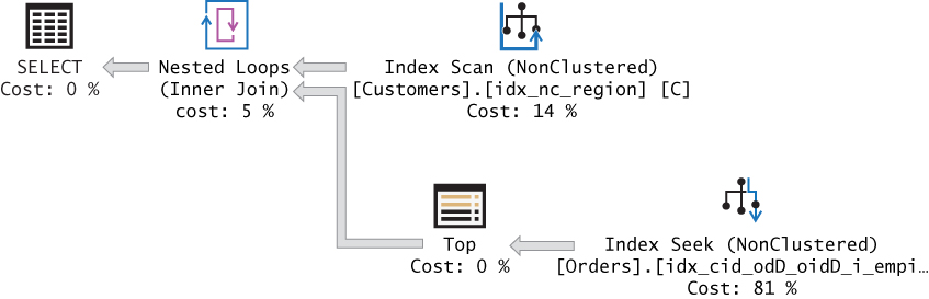
Observe in the plan that an index on the Customers table is scanned to retrieve all customer IDs. Then the plan performs a seek operation for each customer in our POC index going to the beginning of the current customer’s section in the index leaf and scans three rows in the leaf for the three most recent orders.
You can also use the alternative OFFSET-FETCH option instead:
SELECT C.custid, A.orderdate, A.orderid, A.empid
FROM Sales.Customers AS C
  CROSS APPLY (SELECT orderdate, orderid, empid
               FROM Sales.Orders AS O
               WHERE O.custid = C.custid
               ORDER BY orderdate DESC, orderid DESC
               OFFSET 0 ROWS FETCH NEXT 3 ROWS ONLY) AS A;
Note that to perform well, both strategies require a POC index. If you don’t have an index in place and either cannot or do not want to create one, there’s a third strategy that tends to perform better than the other two. However, this third strategy works only when N equals 1.
At this point, you can drop the POC index:
DROP INDEX IF EXISTS idx_cid_odD_oidD_i_empid ON Sales.Orders;
The third strategy implements a carry-along sort technique. I introduced this technique earlier in the book in Chapter 3, “Ordered Set Functions,” when discussing offset functions. The idea is to form a single string for each partition where you first concatenate the ordering attributes and then all the nonkey attributes you need in the result. It’s important to use a concatenation technique that preserves the ordering behavior of the sort elements. For example, in our case, the ordering is based on orderdate DESC and orderid DESC.
The first element is a date. To get a character string representation of a date that sorts the same as the original date, you need to convert the date to the form YYYYMMDD. To achieve this, use the CONVERT function with style 112. As for the orderid element, it’s a positive integer. To have a character string form of the number sort the same as the original integer, you need to format the value as a fixed-length string with leading spaces or zeros. You can format the value as a fixed-length string with leading spaces using the STR function.
The solution involves grouping the rows by the partitioning column and calculating the maximum concatenated string per group. That maximum string represents the concatenated elements from the row you need to return. Next, you define a CTE based on the last query. Then use SUBSTRING functions in the outer query to extract the individual elements you originally concatenated and convert them back to their original types. Here’s what the complete solution looks like:
WITH C AS
(
  SELECT custid,
    MAX(CONVERT(CHAR(8), orderdate, 112)
        + STR(orderid, 10)
        + STR(empid, 10) COLLATE Latin1_General_BIN2) AS mx
  FROM Sales.Orders
  GROUP BY custid
)
SELECT custid,
  CAST(SUBSTRING(mx,  1,  8) AS DATETIME) AS orderdate,
  CAST(SUBSTRING(mx,  9, 10) AS INT)      AS custid,
  CAST(SUBSTRING(mx, 19, 10) AS INT)      AS empid
FROM C;
The query isn’t pretty, but its plan involves only one scan of the data. Also, depending on size, the optimizer can choose between a sort-based and a hash-based aggregate, and it can even parallelize the work. This technique tends to outperform the other solutions when the POC index doesn’t exist. Remember that if you can afford such an index, you don’t want to use this solution; rather, you should use one of the other two strategies, depending on the density of the partitioning column.
Emulating IGNORE NULLS to Get the Last Non-NULL
In Chapter 2, I described the standard null treatment option for window offset functions and mentioned that SQL Server doesn’t support it yet. I used a table called T1 to demonstrate it. Use the following code to create and populate T1 with a small set of sample data:
SET NOCOUNT ON;
USE TSQLV5;

DROP TABLE IF EXISTS dbo.T1;
GO

CREATE TABLE dbo.T1
(
  id INT NOT NULL CONSTRAINT PK_T1 PRIMARY KEY,
  col1 INT NULL
);

INSERT INTO dbo.T1(id, col1) VALUES
  ( 2, NULL),
  ( 3,   10),
  ( 5,   -1),
  ( 7, NULL),
  (11, NULL),
  (13,  -12),
  (17, NULL),
  (19, NULL),
  (23, 1759);
The idea behind the null treatment option is to allow you to control whether to respect NULLs (the default) or ignore NULLs (keep going) when requesting an offset calculation like LAG, LEAD, FIRST_VALUE, LAST_VALUE, and NTH_VALUE. For example, according to the standard, this is how you would ask for the last non-NULL col1 value based on id ordering:
SELECT id, col1,
  COALESCE(col1, LAG(col1) IGNORE NULLS OVER(ORDER BY id)) AS lastval
FROM dbo.T1;
SQL Server doesn’t support this option yet, but here’s the expected result from this query:
id  col1  lastval
--- ----- --------
2   NULL  NULL
3   10    10
5   -1    -1
7   NULL  -1
11  NULL  -1
13  -12   -12
17  NULL  -12
19  NULL  -12
23  1759  1759
In Chapter 2, I presented the following solution (I am referring to it as Solution 1) that does currently work in SQL Server:
WITH C AS
(
  SELECT id, col1,
    MAX(CASE WHEN col1 IS NOT NULL THEN id END)
      OVER(ORDER BY id
           ROWS UNBOUNDED PRECEDING) AS grp
  FROM dbo.T1
)
SELECT id, col1,
  MAX(col1) OVER(PARTITION BY grp
                 ORDER BY id
                 ROWS UNBOUNDED PRECEDING) AS lastval
FROM C;
The inner query in the CTE called C computes for each row a result column called grp representing the last id so far that is associated with a non-NULL col1 value. The first row in each distinct grp group has the last non-NULL value, and the outer query extracts it using a MAX window aggregate that is partitioned by grp.
To test the performance of this solution, you need to populate T1 with a larger set. Use the following code to populate T1 with 10,000,000 rows:
TRUNCATE TABLE dbo.T1;

INSERT INTO dbo.T1 WITH(TABLOCK)
  SELECT n AS id, CHECKSUM(NEWID()) AS col1
  FROM dbo.GetNums(1, 10000000) AS Nums
OPTION(MAXDOP 1);
Use the following code to test Solution 1 using row-mode processing first:
WITH C AS
(
  SELECT id, col1,
    MAX(CASE WHEN col1 IS NOT NULL THEN id END)
      OVER(ORDER BY id
           ROWS UNBOUNDED PRECEDING) AS grp
  FROM dbo.T1
)
SELECT id, col1,
  MAX(col1) OVER(PARTITION BY grp
                 ORDER BY id
                 ROWS UNBOUNDED PRECEDING) AS lastval
FROM C
OPTION(USE HINT('DISALLOW_BATCH_MODE'));
The plan for this query is shown in Figure 6-5.

Observe that the inner window function was computed based on index order, but a sort was needed for the computation of the outer window function. Plus, there are the costs that are associated with the spooling done by the row-mode operators that compute the window aggregate functions. Here are the performance statistics that I got for this solution:
CPU time: 89548 ms, elapsed time: 40319 ms
It took 40 seconds for this solution to complete on my machine.
Test the solution again; this time, allow batch processing (must be in compatibility mode 150 or above, or have a columnstore index present):
WITH C AS
(
  SELECT id, col1,
    MAX(CASE WHEN col1 IS NOT NULL THEN id END)
      OVER(ORDER BY id
           ROWS UNBOUNDED PRECEDING) AS grp
  FROM dbo.T1
)
SELECT id, col1,
  MAX(col1) OVER(PARTITION BY grp
                 ORDER BY id
                 ROWS UNBOUNDED PRECEDING) AS lastval
FROM C;
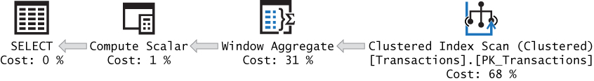
The plan for this execution is shown in Figure 6-6.

As I explained in Chapter 5, when the batch-mode Window Aggregate operator uses parallelism, it cannot rely on index order, so it needs a mediator like a parallel Sort operator. Therefore, you see two Sort operators in the plan. However, this batch-mode operator eliminates a lot of the inefficiencies of the row-mode processing, and it scales so well with multiple CPUs that the performance numbers for this plan are significantly improved:
CPU time: 11609 ms, elapsed time: 5538 ms
Run time dropped by an order of magnitude to only about 6 seconds.
This is great if you’re able to benefit from batch-mode processing. However, if you can’t, there’s another solution that will do better in such a case. For example, you might not be able to benefit from batch-mode processing if you’re running on a version of SQL Server older than 2019 and can’t create a columnstore index—not even a fake filtered one. The second solution uses a carry-along-sort technique, similar to the one you used in the last solution for the Top N Per Group task. Earlier, I showed a technique that uses character string representation of the values. If you’re able to use binary representation, it can be even more efficient because the binary representation tends to be more economic.
Our ordering element is the column id, and it’s a 4-byte positive integer. Internally, SQL Server uses two’s complement representation for integers. Using this format, the binary representation of positive integers preserves the original integer ordering behavior. With this in mind, you can compute a single binary string named binstr that concatenates the binary representation of id and the binary representation of col1 (and any additional columns, if needed). In rows where col1 is NULL, the result binstr is NULL; otherwise, it holds the binary form of the concatenated id and col1 values. Then using a MAX window aggregate, it returns the maximum binstr value so far. The col1 part of the result is the last non-NULL col1 value. Here’s the code implementing this logic:
SELECT id, col1, binstr,
  MAX(binstr) OVER(ORDER BY id ROWS UNBOUNDED PRECEDING) AS mx
FROM dbo.T1
  CROSS APPLY ( VALUES( CAST(id AS BINARY(4)) + CAST(col1 AS BINARY(4)) ) )
    AS A(binstr);
This code generates the following output against the small set of sample data:
id  col1  binstr             mx
--- ----- ------------------ ------------------
2   NULL  NULL               NULL
3   10    0x000000030000000A 0x000000030000000A
5   -1    0x00000005FFFFFFFF 0x00000005FFFFFFFF
7   NULL  NULL               0x00000005FFFFFFFF
11  NULL  NULL               0x00000005FFFFFFFF
13  -12   0x0000000DFFFFFFF4 0x0000000DFFFFFFF4
17  NULL  NULL               0x0000000DFFFFFFF4
19  NULL  NULL               0x0000000DFFFFFFF4
23  1759  0x00000017000006DF 0x00000017000006DF
All that is left is to use the SUBSTRING function to extract the last non-NULL col1 value from the binary string and convert it back to INT, like so (forcing row-mode processing first):
SELECT id, col1,
  CAST( SUBSTRING( MAX( CAST(id AS BINARY(4)) + CAST(col1 AS BINARY(4)) )
                     OVER( ORDER BY id ROWS UNBOUNDED PRECEDING ), 5, 4)
    AS INT) AS lastval
FROM dbo.T1
OPTION(USE HINT('DISALLOW_BATCH_MODE'));
The plan for this query using row-mode processing is shown in Figure 6-7.

Observe that no sorting at all is needed in this plan. Here are the performance statistics that I got for this query:
CPU time: 19282 ms, elapsed time: 19512 ms
Run the query again; this time, allow batch-mode processing:
SELECT id, col1,
  CAST( SUBSTRING( MAX( CAST(id AS BINARY(4)) + CAST(col1 AS BINARY(4)) )
                     OVER( ORDER BY id ROWS UNBOUNDED PRECEDING ), 5, 4)
    AS INT) AS lastval
FROM dbo.T1;
The plan for this query using batch-mode processing is shown in Figure 6-8.

Here are the performance statistics that I got for this query:
CPU time: 16875 ms, elapsed time: 17221 ms
This solution doesn’t perform as well as Solution 1 when using batch mode but does perform much better than when using row-mode processing.
If you’re interested in additional challenges similar to the last non-NULL challenge, you can find those in the following articles:
■ Previous and Next with Condition: https://www.itprotoday.com/sql-server/how-previous-and-next-condition
■ Closest Match, Part 1: https://sqlperformance.com/2018/12/t-sql-queries/closest-match-part-1
■ Closest Match, Part 2: https://sqlperformance.com/2019/01/t-sql-queries/closest-match-part-2
■ Closest Match, Part 3: https://sqlperformance.com/2019/02/t-sql-queries/closest-match-part-3
Mode
Mode is a statistical calculation that returns the most frequently occurring value in the population. Consider, for example, the Sales.Orders table, which holds order information. Each order was placed by a customer and handled by an employee. Suppose you want to know, for each customer, which employee handled the most orders. That employee is the mode because he or she appears most frequently in the customer’s orders.
Naturally, there is the potential for ties if there are multiple employees who handled the most orders for a given customer. Depending on your needs, you either return all ties or break the ties. I will cover solutions to both cases. If you do want to break the ties, suppose the tiebreaker is the highest employee ID number.
Indexing is straightforward here; you want an index defined on (custid, empid):
CREATE INDEX idx_custid_empid ON Sales.Orders(custid, empid);
I’ll start with a solution that relies on the ROW_NUMBER function. The first step is to group the orders by custid and empid and then return for each group the count of orders, like so:
SELECT custid, empid, COUNT(*) AS cnt
FROM Sales.Orders
GROUP BY custid, empid;

custid      empid       cnt
----------- ----------- -----------
1           1           2
3           1           1
4           1           3
5           1           4
9           1           3
10          1           2
11          1           1
14          1           1
15          1           1
17          1           2
...
The next step is to add a ROW_NUMBER calculation partitioned by custid and ordered by COUNT(*) DESC, empid DESC. For each customer, the row with the highest count (and, in the case of ties, the highest employee ID number) will be assigned row number 1:
SELECT custid, empid, COUNT(*) AS cnt,
  ROW_NUMBER() OVER(PARTITION BY custid
                    ORDER BY COUNT(*) DESC, empid DESC) AS rn
FROM Sales.Orders
GROUP BY custid, empid;

custid      empid       cnt         rn
----------- ----------- ----------- --------------------
1           4           2           1
1           1           2           2
1           6           1           3
1           3           1           4
2           3           2           1
2           7           1           2
2           4           1           3
3           3           3           1
3           7           2           2
3           4           1           3
3           1           1           4
...
Finally, you need to filter only the rows where the row number is equal to 1 using a CTE, like so:
WITH C AS
(
  SELECT custid, empid, COUNT(*) AS cnt,
    ROW_NUMBER() OVER(PARTITION BY custid
                      ORDER BY COUNT(*) DESC, empid DESC) AS rn
  FROM Sales.Orders
  GROUP BY custid, empid
)
SELECT custid, empid, cnt
FROM C
WHERE rn = 1;

custid      empid       cnt
----------- ----------- -----------
1           4           2
2           3           2
3           3           3
4           4           4
5           3           6
6           9           3
7           4           3
8           4           2
9           4           4
10          3           4
...
Because the window-ordering specification includes empid DESC as a tiebreaker, you get to return only one row per customer when implementing the tiebreaker requirements of the task. If you do not want to break the ties, use the RANK function instead of ROW_NUMBER and remove empid from the window order clause, like so:
WITH C AS
(
  SELECT custid, empid, COUNT(*) AS cnt,
    RANK() OVER(PARTITION BY custid
                ORDER BY COUNT(*) DESC) AS rk
  FROM Sales.Orders
  GROUP BY custid, empid
)
SELECT custid, empid, cnt
FROM C
WHERE rk = 1;

custid      empid       cnt
----------- ----------- -----------
1           1           2
1           4           2
2           3           2
3           3           3
4           4           4
5           3           6
6           9           3
7           4           3
8           4           2
9           4           4
10          3           4
11          6           2
11          4           2
11          3           2
...
Remember that the RANK function is sensitive to ties, unlike the ROW_NUMBER function. This means that given the same ordering value—COUNT(*) in our case—you get the same rank. So, all rows with the greatest count per customer get rank 1; hence, all are kept. Observe, for example, that in the case of customer 1, two different employees—with IDs 1 and 4—handled the most orders—two in number; hence, both were returned.
Perhaps you realized that the Mode problem is a version of the previously discussed Top-N-per-Group problem. And recall that in addition to the solution that is based on window functions, you can use a solution based on the carry-along-sort concept. However, this concept works only as long as N equals 1, which in our case means you do want to implement a tiebreaker.
To implement the carry-along-sort concept in this case, you need to form a concatenated string with the count as the first part and the employee ID as the second part, like so:
SELECT custid,
  CAST(COUNT(*) AS BINARY(4)) + CAST(empid AS BINARY(4)) AS cntemp
FROM Sales.Orders
GROUP BY custid, empid;

custid      cntemp
----------- ------------------
1           0x0000000200000001
1           0x0000000100000003
1           0x0000000200000004
1           0x0000000100000006
2           0x0000000200000003
2           0x0000000100000004
2           0x0000000100000007
3           0x0000000100000001
3           0x0000000300000003
3           0x0000000100000004
3           0x0000000200000007
...
Because both the count and the employee ID are positive integers, you can concatenate the binary representation of the values, which allows you to preserve their original integer ordering behavior. Alternatively, you could use fixed-length character string segments with leading spaces.
The next step is to define a CTE based on this query, and then in the outer query, group the rows by customer and calculate the maximum concatenated string per group. Finally, extract the different parts from the maximum concatenated string and convert them back to the original types, like so:
WITH C AS
(
  SELECT custid,
    CAST(COUNT(*) AS BINARY(4)) + CAST(empid AS BINARY(4)) AS cntemp
  FROM Sales.Orders
  GROUP BY custid, empid
)
SELECT custid,
  CAST(SUBSTRING(MAX(cntemp), 5, 4) AS INT) AS empid,
  CAST(SUBSTRING(MAX(cntemp),  1, 4) AS INT) AS cnt
FROM C
GROUP BY custid;

custid      empid       cnt
----------- ----------- -----------
1           4           2
2           3           2
3           3           3
4           4           4
5           3           6
6           9           3
7           4           3
8           4           2
9           4           4
10          3           4
...
As mentioned in the “TOP N per Group” section, the solution based on window functions performs well when there is an index in place, so there’s no reason to use the more complicated carry-along-sort solution. But when there’s no supporting index, the carry-along-sort solution tends to perform better.
When you’re done, run the following code for cleanup:
DROP INDEX IF EXISTS idx_custid_empid ON Sales.Orders;
Trimmed Mean
Trimmed mean is a statistical calculation of the average of some measure after removing a certain fixed percent of the bottom and top samples, which are considered outliers.
For example, suppose that you need to query the Sales.OrderValues view and return the average of the order values per employee, excluding the bottom and top 5 percent of the order values for each employee. This can be done easily with the help of the NTILE function. Using this function, you bucketize the samples in percent groups. For instance, to arrange the orders per employee in 5-percent groups, compute NTILE(20), like so:
SELECT empid, val,
  NTILE(20) OVER(PARTITION BY empid ORDER BY val) AS ntile20
FROM Sales.OrderValues;
This query generates the following output for employee 1 (abbreviated):
empid  val       ntile20
------ --------- --------
1      33.75     1
1      69.60     1
1      72.96     1
1      86.85     1
1      93.50     1
1      108.00    1
1      110.00    1
1      137.50    2
1      147.00    2
1      154.40    2
1      230.40    2
1      230.85    2
1      240.00    2
1      268.80    2
...
1      3192.65   19
1      3424.00   19
1      3463.00   19
1      3687.00   19
1      3868.60   19
1      4109.70   19
1      4330.40   20
1      4807.00   20
1      5398.73   20
1      6375.00   20
1      6635.28   20
1      15810.00  20
...
To remove the bottom and top 5 percent of the orders per employee, place the last query in a CTE; in the outer query filter tiles 2 through 19, group the remaining rows by the employee ID. Finally, compute the average of the remaining order values per employee. Here’s the complete solution query:
WITH C AS
(
  SELECT empid, val,
    NTILE(20) OVER(PARTITION BY empid ORDER BY val) AS ntile20
  FROM Sales.OrderValues
)
SELECT empid, AVG(val) AS avgval
FROM C
WHERE ntile20 BETWEEN 2 AND 19
GROUP BY empid;
This code generates the following output:
empid  avgval
------ ------------
1      1347.059818
2      1389.643793
3      1269.213508
4      1314.047234
5      1424.875675
6      1048.360166
7      1444.162307
8      1135.191827
9      1554.841578
Running Totals
Calculating running totals is a very common need. The basic idea is to keep accumulating the values of some measure based on some ordering element, possibly within partitions of rows. There are many practical examples for calculating running totals, including calculating bank account balances, tracking product stock levels in a warehouse, tracking cumulative sales values, and so on.
Without window functions, set-based solutions to calculate running totals are extremely expensive. Therefore, before window functions with a frame were introduced in SQL Server, people often resorted to iterative solutions that weren’t very fast but in certain data distribution scenarios were faster than the set-based solutions. With window functions you can calculate running totals with simple set-based code that performs much better than all the alternative T-SQL solutions—set-based and iterative. I could have just showed you the code with the window function and moved on to the next topic, but to help you really appreciate the greatness of window functions and how they get optimized, I will also describe the alternatives—though inferior—and provide a performance comparison between the solutions. Feel free, of course, to read only the first section covering the window function and skip the rest if that’s what you prefer.
I will compare solutions for computing bank account balances as my example for a running totals task. Listing 6-3 provides code you can use to create and populate the Transactions table with a small set of sample data.
LISTING 6-3 Create and Populate the Transactions Table with a Small Set of Sample Data
SET NOCOUNT ON;
USE TSQLV5;

DROP TABLE IF EXISTS dbo.Transactions;

CREATE TABLE dbo.Transactions
(
  actid  INT   NOT NULL,                -- partitioning column
  tranid INT   NOT NULL,                -- ordering column
  val    MONEY NOT NULL,                -- measure
  CONSTRAINT PK_Transactions PRIMARY KEY(actid, tranid)
);
GO

-- small set of sample data
INSERT INTO dbo.Transactions(actid, tranid, val) VALUES
  (1,  1,  4.00),
  (1,  2, -2.00),
  (1,  3,  5.00),
  (1,  4,  2.00),
  (1,  5,  1.00),
  (1,  6,  3.00),
  (1,  7, -4.00),
  (1,  8, -1.00),
  (1,  9, -2.00),
  (1, 10, -3.00),
  (2,  1,  2.00),
  (2,  2,  1.00),
  (2,  3,  5.00),
  (2,  4,  1.00),
  (2,  5, -5.00),
  (2,  6,  4.00),
  (2,  7,  2.00),
  (2,  8, -4.00),
  (2,  9, -5.00),
  (2, 10,  4.00),
  (3,  1, -3.00),
  (3,  2,  3.00),
  (3,  3, -2.00),
  (3,  4,  1.00),
  (3,  5,  4.00),
  (3,  6, -1.00),
  (3,  7,  5.00),
  (3,  8,  3.00),
  (3,  9,  5.00),
  (3, 10, -3.00);
Each row in the table represents a transaction in some bank account. When the transaction is a deposit, the amount in the val column is positive; when it’s a withdrawal, the amount is negative. Your task is to compute the account balance at each point by accumulating the amounts in the val column based on ordering defined by the tranid column within each account independently. The desired results for the small set of sample data should look like Listing 6-4.
LISTING 6-4 Desired Results for Running Totals Task
actid       tranid      val                   balance
----------- ----------- --------------------- ---------------------
1           1           4.00                  4.00
1           2           -2.00                 2.00
1           3           5.00                  7.00
1           4           2.00                  9.00
1           5           1.00                  10.00
1           6           3.00                  13.00
1           7           -4.00                 9.00
1           8           -1.00                 8.00
1           9           -2.00                 6.00
1           10          -3.00                 3.00
2           1           2.00                  2.00
2           2           1.00                  3.00
2           3           5.00                  8.00
2           4           1.00                  9.00
2           5           -5.00                 4.00
2           6           4.00                  8.00
2           7           2.00                  10.00
2           8           -4.00                 6.00
2           9           -5.00                 1.00
2           10          4.00                  5.00
3           1           -3.00                 -3.00
3           2           3.00                  0.00
3           3           -2.00                 -2.00
3           4           1.00                  -1.00
3           5           4.00                  3.00
3           6           -1.00                 2.00
3           7           5.00                  7.00
3           8           3.00                  10.00
3           9           5.00                  15.00
3           10          -3.00                 12.00
To test the performance of the solutions, you need a larger set of sample data. You can use the following code to achieve this:
DECLARE
  @num_partitions     AS INT = 100,
  @rows_per_partition AS INT = 10000;

TRUNCATE TABLE dbo.Transactions;

INSERT INTO dbo.Transactions WITH (TABLOCK) (actid, tranid, val)
  SELECT NP.n, RPP.n,
    (ABS(CHECKSUM(NEWID())%2)*2-1) * (1 + ABS(CHECKSUM(NEWID())%5))
  FROM dbo.GetNums(1, @num_partitions) AS NP
    CROSS JOIN dbo.GetNums(1, @rows_per_partition) AS RPP;
Feel free to change the inputs as needed to control the number of partitions (accounts) and number of rows per partition (transactions).
Set-Based Solution Using Window Functions
I’ll start with the most optimal set-based solution that uses the SUM window aggregate function. The window specification is intuitive here; you need to partition the window by actid, order by tranid, and filter the frame of rows between no low boundary point (UNBOUNDED PRECEDING) and the current row. Here’s the solution query:
SELECT actid, tranid, val,
  SUM(val) OVER(PARTITION BY actid
                ORDER BY tranid
                ROWS UNBOUNDED PRECEDING) AS balance
FROM dbo.Transactions;
Not only is the code simple and straightforward, it also performs very well. The plan for this query is shown in Figure 6-9.
The table has a clustered index that follows the POC guidelines that window functions can benefit from. Namely, the index key list is based on the partitioning element (actid) followed by the ordering element (tranid), and it includes for coverage purposes all the rest of the columns in the query (val). The plan shows an ordered scan of the index, followed by the computation of the running total with the batch-mode Window Aggregate operator. Because you arranged a POC index, the optimizer didn’t need to add a sort operator in the plan. That’s a very efficient plan. It took less than half a second to complete on my machine against a table with 1,000,000 rows, and the results were discarded. What’s more, this plan scales linearly.
Set-Based Solutions Using Subqueries or Joins
Traditional set-based solutions to running totals that don’t use window functions use either subqueries or joins. Using a subquery, you can calculate the running total by filtering all rows that have the same actid value as in the outer row and a tranid value that is less than or equal to the one in the outer row. Then you apply the aggregate to the filtered rows. Here’s the solution query:
SELECT actid, tranid, val,
  (SELECT SUM(T2.val)
   FROM dbo.Transactions AS T2
   WHERE T2.actid = T1.actid
     AND T2.tranid <= T1.tranid) AS balance
FROM dbo.Transactions AS T1;
A similar approach can be implemented using joins. You use the same predicate as the one used in the WHERE clause of the subquery in the ON clause of the join. This way, for the Nth transaction of account A in the instance you refer to as T1, you will find N matches in the instance T2 with transactions 1 through N. The row in T1 is repeated in the result for each of its matches, so you need to group the rows by all elements from T1 to get the current transaction info and apply the aggregate to the val attribute from T2 to calculate the running total. The solution query looks like this:
SELECT T1.actid, T1.tranid, T1.val,
  SUM(T2.val) AS balance
FROM dbo.Transactions AS T1
  INNER JOIN dbo.Transactions AS T2
    ON T2.actid = T1.actid
   AND T2.tranid <= T1.tranid
GROUP BY T1.actid, T1.tranid, T1.val;
Figure 6-10 shows the plans for both solutions.

Observe that in both cases, the clustered index is scanned in full representing the instance T1. The plan performs a seek operation for each row in the index to get to the beginning of the current account’s section in the index leaf, and then it scans all transactions where T2.tranid is less than or equal to T1.tranid. Then the point where the aggregate of those rows takes place is a bit different in the two plans, but the number of rows scanned is the same. Also, it appears that the optimizer chose a parallel plan for the subquery solution and a serial plan for the join solution.
To realize how many rows get scanned, consider the elements involved in the data. Let p be the number of partitions (accounts), and let r be the number of rows per partition (transactions). Then the number of rows in the table is roughly pr, assuming an even distribution of transactions per account. So, the upper scan of the clustered index involves scanning pr rows. But the work at the inner part of the Nested Loops operator is what we’re most concerned with. For each partition, the plan scans 1 + 2 + … + r rows, which is equal to (r + r^2) / 2. In total, the number of rows processed in these plans is pr + p(r + r^2) / 2. This means that with respect to partition size, the scaling of this plan is quadratic (N^2); that is, if you increase the partition size by a factor of f, the work involved increases by a factor of close to f^2. That’s bad. As examples, for a partition of 100 rows, the plan touches 5,050 rows. For a partition of 10,000 rows, the plan processes 50,005,000 rows, and so on. Simply put, it translates to very slow queries when the partition size is not tiny because the squared effect is very dramatic. It’s okay to use these solutions for up to a few dozen rows per partition but not many more.
As an example, the subquery solution took 10 minutes to complete on my machine against a table with 1,000,000 rows (100 accounts, each with 10,000 transactions). Remember, the query with the window function completed in less than half a second against the same data!
Cursor-Based Solution
Using a cursor-based solution to running totals is straightforward. You declare a cursor based on a query that orders the data by actid and tranid. You then iterate through the cursor records. When you hit a new account, you reset the variable holding the aggregate. In each iteration, you add the value of the new transaction to the variable; you then store a row in a table variable with the current transaction information plus the running total so far. When you’re done iterating, you return the result to the caller by querying the table variable. Listing 6-5 shows the complete solution code.
LISTING 6-5 Cursor-Based Solution for Running Totals
DECLARE @Result AS TABLE
(
  actid   INT,
  tranid  INT,
  val     MONEY,
  balance MONEY
);

DECLARE
  @C        AS CURSOR,
  @actid    AS INT,
  @prvactid AS INT,
  @tranid   AS INT,
  @val      AS MONEY,
  @balance  AS MONEY;

SET @C = CURSOR FORWARD_ONLY STATIC READ_ONLY FOR
  SELECT actid, tranid, val
  FROM dbo.Transactions
  ORDER BY actid, tranid;

OPEN @C

FETCH NEXT FROM @C INTO @actid, @tranid, @val;

SELECT @prvactid = @actid, @balance = 0;

WHILE @@fetch_status = 0
BEGIN
  IF @actid <> @prvactid
    SELECT @prvactid = @actid, @balance = 0;

  SET @balance = @balance + @val;

  INSERT INTO @Result VALUES(@actid, @tranid, @val, @balance);

  FETCH NEXT FROM @C INTO @actid, @tranid, @val;
END

SELECT * FROM @Result;
The plan for the query that the cursor is based on is shown in Figure 6-11.

This plan has linear scaling because the data from the index is scanned only once, in order. Also, each fetching of a row from the cursor has a constant cost per row. If you call the cursor overhead per row o, you can express the cost of this solution as pr + pro. (Keep in mind that p is the number of partitions and r is the number of rows per partition.) So, you can see that if you increase the number of rows per partition by a factor of f, the work involved becomes prf + prfo, meaning that you get linear scaling. The overhead per row is high; however, because the scaling is linear, from a certain partition size and on this solution will perform better than the solutions based on subqueries and joins because of their quadratic scaling. Performance tests that I did show that the point where the cursor solution becomes faster is around a few hundred rows per partition.
It took the cursor solution 31 seconds to complete on my machine against a table with 1,000,000 rows.
CLR-Based Solution
One possible Common Language Runtime (CLR) solution is basically another form of a cursor-based solution. The difference is that instead of using a T-SQL cursor that involves a high amount of overhead for each fetch and slow iterations, you use a .NET SQLDataReader and .NET iterations, which are much faster. Furthermore, you don’t need to store the result rows in a temporary table—the results are streamed right back to the caller. The logic of the CLR-based solution is similar to that of the T-SQL cursor-based solution. Listing 6-6 shows the .NET code defining the solution’s stored procedure.
LISTING 6-6 CLR-Based Solution for Running Totals
using System;
using System.Data;
using System.Data.SqlClient;
using System.Data.SqlTypes;
using Microsoft.SqlServer.Server;

public partial class StoredProcedures
{
    [Microsoft.SqlServer.Server.SqlProcedure]
    public static void AccountBalances()
    {
        using (SqlConnection conn = new SqlConnection("context connection=true;"))
        {
            SqlCommand comm = new SqlCommand();
            comm.Connection = conn;
            comm.CommandText = @"" +
                "SELECT actid, tranid, val " +
                "FROM dbo.Transactions " +
                "ORDER BY actid, tranid;";

            SqlMetaData[] columns = new SqlMetaData[4];
            columns[0] = new SqlMetaData("actid"  , SqlDbType.Int);
            columns[1] = new SqlMetaData("tranid" , SqlDbType.Int);
            columns[2] = new SqlMetaData("val"    , SqlDbType.Money);
            columns[3] = new SqlMetaData("balance", SqlDbType.Money);

            SqlDataRecord record = new SqlDataRecord(columns);
            SqlContext.Pipe.SendResultsStart(record);

            conn.Open();

            SqlDataReader reader = comm.ExecuteReader();

            SqlInt32 prvactid = 0;
            SqlMoney balance = 0;

            while (reader.Read())
            {
                SqlInt32 actid = reader.GetSqlInt32(0);
                SqlMoney val = reader.GetSqlMoney(2);

                if (actid == prvactid)
                {
                    balance += val;
                }
                else
                {
                    balance = val;
                }

                prvactid = actid;

                record.SetSqlInt32(0, reader.GetSqlInt32(0));
                record.SetSqlInt32(1, reader.GetSqlInt32(1));
                record.SetSqlMoney(2, val);
                record.SetSqlMoney(3, balance);

                SqlContext.Pipe.SendResultsRow(record);
            }

            SqlContext.Pipe.SendResultsEnd();
        }
    }
};
To be able to execute the stored procedure in SQL Server, you first need to build an assembly called AccountBalances that is based on this code and deploy it in the TSQLV5 database.
Note If you’re not familiar with deployment of assemblies in SQL Server, you can read about it in T-SQL Querying (Microsoft Press). Also, see the Microsoft article, “Deploying CLR Database Objects,” at https://docs.microsoft.com/en-us/sql/relational-databases/clr-integration/deploying-clr-database-objects.
Assuming you called the assembly AccountBalances, and the path to the assembly file is C:AccountBalancesAccountBalances.dll, you can use the following code to load the assembly to the database and then register the stored procedure:
CREATE ASSEMBLY AccountBalances FROM 'C:AccountBalancesAccountBalances.dll';
GO
CREATE PROCEDURE dbo.AccountBalances
AS EXTERNAL NAME AccountBalances.StoredProcedures.AccountBalances;
After the assembly has been deployed and the procedure has been registered, you can execute the procedure using the following code:
EXEC dbo.AccountBalances;
As mentioned, a SQLDataReader is just another form of a cursor, only the overhead of each fetch is less than that of a T-SQL cursor. Also, iterations in .NET are much faster than iterations in T-SQL. So, the CLR-based solution also has linear scaling. In my benchmarks, this solution started performing better than the solutions using subqueries and joins at around 15 rows per partition. It took this stored procedure 3.8 seconds to complete against a table with 1,000,000 rows.
When you’re done, run the following code for cleanup:
DROP PROCEDURE IF EXISTS dbo.AccountBalances;
DROP ASSEMBLY IF EXISTS AccountBalances;
Nested Iterations
So far, I have shown you solutions that are either set based or iterative. The next solution, known as nested iterations, is a hybrid of iterative and set-based logic. The idea is to first copy the rows from the source table (bank account transactions in our case) into a temporary table, along with a new attribute called rownum that is calculated by using the ROW_NUMBER function. The row numbers are partitioned by actid and ordered by tranid, so the first transaction in each account is assigned the row number 1, the second transaction is assigned row number 2, and so on. You then create a clustered index on the temporary table with the key list (rownum, actid). Then you use either a recursive CTE or your own loop to handle one row number at a time across all accounts in each iteration. The running total is then computed by adding the value associated with the current row number to the value associated with the previous row number.
Listing 6-7 shows the implementation of this logic using a recursive CTE.
LISTING 6-7 Solution with Recursive CTE to Running Totals
SELECT actid, tranid, val,
  ROW_NUMBER() OVER(PARTITION BY actid ORDER BY tranid) AS rownum
INTO #Transactions
FROM dbo.Transactions;

CREATE UNIQUE CLUSTERED INDEX idx_rownum_actid ON #Transactions(rownum, actid);

WITH C AS
(
  SELECT 1 AS rownum, actid, tranid, val, val AS sumqty
  FROM #Transactions
  WHERE rownum = 1

  UNION ALL

  SELECT PRV.rownum + 1, PRV.actid, PRV.tranid, CUR.val, PRV.sumqty + CUR.val
  FROM C AS PRV
    INNER JOIN #Transactions AS CUR
      ON CUR.rownum = PRV.rownum + 1
      AND CUR.actid = PRV.actid
)
SELECT actid, tranid, val, sumqty
FROM C
OPTION (MAXRECURSION 0);

DROP TABLE IF EXISTS #Transactions;
And here’s the implementation of the same logic using an explicit loop:
SELECT ROW_NUMBER() OVER(PARTITION BY actid ORDER BY tranid) AS rownum,
  actid, tranid, val, CAST(val AS BIGINT) AS sumqty
INTO #Transactions
FROM dbo.Transactions;

CREATE UNIQUE CLUSTERED INDEX idx_rownum_actid ON #Transactions(rownum, actid);

DECLARE @rownum AS INT;
SET @rownum = 1;

WHILE 1 = 1
BEGIN
  SET @rownum = @rownum + 1;

  UPDATE CUR
    SET sumqty = PRV.sumqty + CUR.val
  FROM #Transactions AS CUR
    INNER JOIN #Transactions AS PRV
      ON CUR.rownum = @rownum
     AND PRV.rownum = @rownum - 1
     AND CUR.actid = PRV.actid;

  IF @@rowcount = 0 BREAK;
END

SELECT actid, tranid, val, sumqty
FROM #Transactions;

DROP TABLE IF EXISTS #Transactions;
This solution tends to perform well when there are a lot of partitions with a small number of rows per partition. This means the number of iterations is small. And most of the work is handled by the set-based part of the solution that joins the rows associated with one row number with the rows associated with the previous row number.
Using the same data with 1,000,000 rows (100 accounts, each with 10,000 transactions), the code with the recursive query took 16 seconds to complete, and the code with the loop took 7 seconds to complete.
Multirow UPDATE with Variables
The various techniques I showed so far for handling running totals are guaranteed to produce the correct result. The technique that is the focus of this section is a controversial one because it relies on observed behavior as opposed to documented behavior, and it violates relational concepts. What makes it so appealing to some is that it is very fast, though it’s still slower than a simple windowed running sum.
The technique involves using an UPDATE statement with variables. An UPDATE statement can set a variable to an expression based on a column value, as well as set a column value to an expression based on a variable. The solution starts by creating a temporary table called #Transactions with the actid, tranid, val, and balance attributes and a clustered index based on the key list (actid, tranid). Then the solution populates the temp table with all rows from the source Transactions table, setting the balance column to 0.00 in all rows. The solution then invokes an UPDATE statement with variables against the temporary table to calculate the running totals and assign those to the balance column. It uses variables called @prevaccount and @prevbalance, and it sets the balance using the following expression:
SET @prevbalance = balance = CASE
                                 WHEN actid = @prevaccount
                                   THEN @prevbalance + val
                                 ELSE val
                               END
The CASE expression checks whether the current account ID is equal to the previous account ID; if the account IDs are equivalent, it returns the previous balance plus the current transaction value. If the account IDs are different, it returns the current transaction value. The balance is then set to the result of the CASE expression and assigned to the @prevbalance variable. In a separate expression, the @prevaccount variable is set to the current account ID.
After the UPDATE statement, the solution presents the rows from the temporary table and then drops the table. Listing 6-8 shows the complete solution code.
LISTING 6-8 Solution Using Multirow UPDATE with Variables
CREATE TABLE #Transactions
(
  actid          INT,
  tranid         INT,
  val            MONEY,
  balance        MONEY
);

CREATE CLUSTERED INDEX idx_actid_tranid ON #Transactions(actid, tranid);

INSERT INTO #Transactions WITH (TABLOCK) (actid, tranid, val, balance)
  SELECT actid, tranid, val, 0.00
  FROM dbo.Transactions
  ORDER BY actid, tranid;

DECLARE @prevaccount AS INT, @prevbalance AS MONEY;

UPDATE #Transactions
  SET @prevbalance = balance = CASE
                                 WHEN actid = @prevaccount
                                   THEN @prevbalance + val
                                 ELSE val
                               END,
      @prevaccount = actid
FROM #Transactions WITH(INDEX(1), TABLOCKX)
OPTION (MAXDOP 1);

SELECT * FROM #Transactions;

DROP TABLE IF EXISTS #Transactions;
The plan for this solution is shown in Figure 6-12. The first part is the INSERT, the second part is the UPDATE, and the third part is the SELECT.

It took this solution close to 3 seconds to complete on my machine.
This solution makes an assumption that the UPDATE will always be optimized with an ordered scan of the clustered index, and it even uses a number of hints in an attempt to avoid situations that might prevent that—for example, parallelism. The problem is that there is no official guarantee that the optimizer will always scan the data in clustered index order. You’re not supposed to make assumptions about physical processing aspects when trying to ensure the logical correctness of your code, unless there are logical elements in the code that are defined to guarantee such behavior. There’s nothing in the logical aspects of the code that give any such guarantees. Of course, it’s up to you to decide whether or not you want to use this technique. I think it’s irresponsible to use it even if you run it a thousand times and the observed behavior is “It seems to work.” The reason I’m covering it in the book is because it is being used out there in the wild, you might stumble into it, but I wanted to make sure to warn you against using it.
Fortunately, the solution using the window aggregate function is so much faster than any other solution, including this one, that it should be the preferred choice anyway.
Performance Benchmark
I ran a performance benchmark comparing the different techniques. Figures 6-13 and 6-14 show the results of that benchmark.


The reason for separating the results into two graphs was that the technique based on a subquery or join was so slow compared to the rest that I wanted to use a different scale for it. Regardless of the reason for doing it this way, observe that with respect to partition size, most solutions have linear scaling, and only the one based on a subquery or join has quadratic scaling. Also, you can clearly see how efficient the solution based on a window aggregate function is. The solution based on an UPDATE with variables is also very fast, but for the aforementioned reasons I recommended that you avoid it. The solution based on the CLR is also quite fast, but it involves writing all that .NET code and deploying an assembly in the database. From all perspectives, the set-based solution using a window aggregate is by far the most preferable one.
Here, I showed a basic form of running totals. In subsequent sections, I show more sophisticated uses of running totals in more complex scenarios.
Max Concurrent Intervals
Consider a set of intervals representing things such as sessions, validity periods, contract periods, drug prescription periods, and so on. There’s a classic task known as maximum concurrent intervals where you’re after the maximum number of intervals that were active concurrently. As an example, suppose that you’re given a table called Sessions that holds data about user sessions against different applications. Your task is to write a solution that calculates, for each application, the maximum number of sessions that were active at any given point in time. If one session ends exactly when another starts, assume that you’re not supposed to consider them concurrent. In other words, consider the intervals as closed-open intervals.
Here’s the code to create the Sessions table:
SET NOCOUNT ON;
USE TSQLV5;

DROP TABLE IF EXISTS dbo.Sessions;

CREATE TABLE dbo.Sessions
(
  keycol    INT          NOT NULL,
  app       VARCHAR(10)  NOT NULL,
  usr       VARCHAR(10)  NOT NULL,
  host      VARCHAR(10)  NOT NULL,
  starttime DATETIME2(0) NOT NULL,
  endtime   DATETIME2(0) NOT NULL,
  CONSTRAINT PK_Sessions PRIMARY KEY(keycol),
  CHECK(endtime > starttime)
);
GO
Use the following code to populate the Sessions table with a small set of sample data to test the validity of your solution:
TRUNCATE TABLE dbo.Sessions;

INSERT INTO dbo.Sessions(keycol, app, usr, host, starttime, endtime) VALUES
  (2,  'app1', 'user1', 'host1', '20190212 08:30', '20190212 10:30'),
  (3,  'app1', 'user2', 'host1', '20190212 08:30', '20190212 08:45'),
  (5,  'app1', 'user3', 'host2', '20190212 09:00', '20190212 09:30'),
  (7,  'app1', 'user4', 'host2', '20190212 09:15', '20190212 10:30'),
  (11, 'app1', 'user5', 'host3', '20190212 09:15', '20190212 09:30'),
  (13, 'app1', 'user6', 'host3', '20190212 10:30', '20190212 14:30'),
  (17, 'app1', 'user7', 'host4', '20190212 10:45', '20190212 11:30'),
  (19, 'app1', 'user8', 'host4', '20190212 11:00', '20190212 12:30'),
  (23, 'app2', 'user8', 'host1', '20190212 08:30', '20190212 08:45'),
  (29, 'app2', 'user7', 'host1', '20190212 09:00', '20190212 09:30'),
  (31, 'app2', 'user6', 'host2', '20190212 11:45', '20190212 12:00'),
  (37, 'app2', 'user5', 'host2', '20190212 12:30', '20190212 14:00'),
  (41, 'app2', 'user4', 'host3', '20190212 12:45', '20190212 13:30'),
  (43, 'app2', 'user3', 'host3', '20190212 13:00', '20190212 14:00'),
  (47, 'app2', 'user2', 'host4', '20190212 14:00', '20190212 16:30'),
  (53, 'app2', 'user1', 'host4', '20190212 15:30', '20190212 17:00');
Here’s the desired result for this small set of sample data:
app         mx
---------- -----------
app1       4
app2       3
To test the performance of your solution, you need a larger set of sample data. The following code populates the table with 1,000,000 sessions with 10 distinct applications:
TRUNCATE TABLE dbo.Sessions;

DECLARE
  @numrows AS INT = 1000000, -- total number of rows
  @numapps AS INT = 10;      -- number of applications

INSERT INTO dbo.Sessions WITH(TABLOCK)
    (keycol, app, usr, host, starttime, endtime)
  SELECT
    ROW_NUMBER() OVER(ORDER BY (SELECT NULL)) AS keycol,
    D.*,
    DATEADD(
      second,
      1 + ABS(CHECKSUM(NEWID())) % (20*60),
      starttime) AS endtime
  FROM
  (
    SELECT
      'app' + CAST(1 + ABS(CHECKSUM(NEWID())) % @numapps AS VARCHAR(10)) AS app,
      'user1' AS usr,
      'host1' AS host,
      DATEADD(
        second,
        1 + ABS(CHECKSUM(NEWID())) % (30*24*60*60),
        '20190101') AS starttime
    FROM dbo.GetNums(1, @numrows) AS Nums
  ) AS D;
Feel free to adjust the number of rows to populate the table with and the number of distinct applications according to your needs.
Before I show the efficient solutions that are based on window functions, I’ll show a couple of solutions that do not use window functions and talk about their shortcomings. I’ll first describe the traditional set-based solution.
Traditional Set-Based Solution
You can think of each session as being made of two events—a start event, which increases the count of active sessions, and an end event, which decreases that count. If you look at the timeline, the count of active sessions remains constant in sections between consecutive events where a session either starts or ends. What’s more, because a start event increases the count of active sessions, the maximum count must fall on a start event. As an example, suppose that there were two sessions with a certain application named App1: one session started at point P1 and ended at point P3, and another session started at point P2 and ended at point P4. Here’s the chronological order of events and the number of active sessions after each event:
■ P1, session 1 starts, 1 active session
■ P2, session 2 starts, 2 active sessions
■ P3, session 1 ends, 1 active session
■ P4, session 2 ends, 0 active sessions
The number of active sessions between two consecutive points remains constant. The maximum number falls on a start point—P2 in this example.
The approach taken by the traditional set-based solution relies on this logic. The solution implements the following steps:
1. Define a table expression called TimePoints based on a query against the Sessions table that returns app and starttime (aliased as ts for timestamp).
2. Use a second table expression called Counts to query TimePoints (aliased as P).
3. In the second table expression, use a subquery to count how many sessions you can find in the Sessions table (aliased as S), where P.app is equal to S.app, and P.ts is on or after S.starttime and before S.endtime. The subquery counts how many sessions are active during each application session’s start point in time.
4. Finally, in the outer query against Counts, group the rows by app and return the maximum count for each application.
Here’s the complete solution code:
WITH TimePoints AS
(
  SELECT app, starttime AS ts FROM dbo.Sessions
),
Counts AS
(
  SELECT app, ts,
    (SELECT COUNT(*)
     FROM dbo.Sessions AS S
     WHERE P.app = S.app
       AND P.ts >= S.starttime
       AND P.ts < S.endtime) AS concurrent
  FROM TimePoints AS P
)
SELECT app, MAX(concurrent) AS mx
FROM Counts
GROUP BY app;
Use the following code to create an index that supports this solution:
CREATE INDEX idx_start_end ON dbo.Sessions(app, starttime, endtime);
The solution seems straightforward, and it might not be immediately apparent that there’s a performance problem with it. However, when you run it against the large set of sample data, it takes a long time to complete. To understand why it’s so slow, examine the query’s execution plan, as shown in Figure 6-15.

The Index Scan operator in the top-right part of the plan (the outer input of the Nested Loops join) scans the index you created earlier (idx_start_end) to obtain all start points per application. Using the symbols p for the number of partitions (applications) and r for the number of rows per partition (sessions per application), this part involves scanning roughly pr rows. Then the inner part of the Nested Loops join is an Index Seek operator against the same index that gets executed for each row returned from the upper input. Its task is to identify the rows representing the sessions that were active for the current application during the current point in time in the outer row.
Think about the work involved in each execution of the Index Seek operator. For the current outer row’s elements P.app (call it myapp) and P.ts (call it myts), the operator is looking for all rows where S.app = myapp, and S.starttime <= myts, and S.endtime > myts. The seek predicates can be applied based on any number of leading elements in the index key that appear in equality predicates (S.app = myapp, in our case), followed by one more element that appears in a range predicate (S.starttime <= myts, in our case). Only the qualifying rows that satisfy the seek predicates have to be read. However, if there are additional range predicates (S.endtime > myts, in our case), they are applied as residual predicates, meaning that both qualifying and nonqualifying rows have to be read, and based on the outcome of the predicate, only the qualifying rows are actually returned. Observe in Figure 6-15 that you can see which predicates are applied as Seek Predicates versus (residual) Predicate in the Index Seek operator’s properties.
If it isn’t clear by now, that’s bad news. Whereas the seek predicate prevents reading nonqualifying rows, the residual predicate doesn’t. I already mentioned that the Index Scan operator scans approximately pr rows. The Index Seek operator scans, for each row, on average about half the rows in the partition. This means that for r rows in a partition, it scans r^2 / 2 rows. In total, the number of rows being touched is pr + pr^2 / 2. This means that with respect to partition size, this plan has quadratic complexity. So, if the number of rows per partition increases by a factor of f, the work increases by a factor of close to f^2. So, beyond very small partition sizes, the query will perform very badly. It took this query more than an hour to complete on my machine with 1,000,000 rows in the table.
When you’re done, run the following code to drop the index you created to support this solution:
DROP INDEX IF EXISTS idx_start_end ON dbo.Sessions;
Solutions Based on Window Functions
I’ll present two solutions based on window functions—one using running totals and another using row numbers. Both solutions benefit from the following indexes that separate session start and end events:
CREATE UNIQUE INDEX idx_start ON dbo.Sessions(app, starttime, keycol);
CREATE UNIQUE INDEX idx_end ON dbo.Sessions(app, endtime, keycol);
The first solution starts by producing a chronological sequence of session start and end events, using the following code (shown here ordered):
SELECT keycol, app, starttime AS ts, +1 AS type
FROM dbo.Sessions

UNION ALL

SELECT keycol, app, endtime AS ts, -1 AS type
FROM dbo.Sessions

ORDER BY app, ts, type, keycol;
Observe that start events are marked with a +1 event type because they increase the count of active sessions, and end events are marked with −1 because they decrease the count. The presentation ORDER BY clause is used here, for illustration purposes, to show the events in chronological order. Within each application, the events are ordered by the time stamp (ts), then by type. The reason to add type to the ordering is so that if one session ends exactly where another starts, the −1 will appear before the +1, and this way the two will not be considered concurrent. Finally, keycol is added at the end of the ordering just for determinism.
This code generates the output shown in Listing 6-9 using the small set of sample data.
LISTING 6-9 Chronological Sequence of Session Start and End Events
keycol  app   ts                   type
------- ----- -------------------- -----
2       app1  2019-02-12 08:30:00  1
3       app1  2019-02-12 08:30:00  1
3       app1  2019-02-12 08:45:00  -1
5       app1  2019-02-12 09:00:00  1
7       app1  2019-02-12 09:15:00  1
11      app1  2019-02-12 09:15:00  1
5       app1  2019-02-12 09:30:00  -1
11      app1  2019-02-12 09:30:00  -1
2       app1  2019-02-12 10:30:00  -1
7       app1  2019-02-12 10:30:00  -1
13      app1  2019-02-12 10:30:00  1
17      app1  2019-02-12 10:45:00  1
19      app1  2019-02-12 11:00:00  1
17      app1  2019-02-12 11:30:00  -1
19      app1  2019-02-12 12:30:00  -1
13      app1  2019-02-12 14:30:00  -1
23      app2  2019-02-12 08:30:00  1
23      app2  2019-02-12 08:45:00  -1
29      app2  2019-02-12 09:00:00  1
29      app2  2019-02-12 09:30:00  -1
31      app2  2019-02-12 11:45:00  1
31      app2  2019-02-12 12:00:00  -1
37      app2  2019-02-12 12:30:00  1
41      app2  2019-02-12 12:45:00  1
43      app2  2019-02-12 13:00:00  1
41      app2  2019-02-12 13:30:00  -1
37      app2  2019-02-12 14:00:00  -1
43      app2  2019-02-12 14:00:00  -1
47      app2  2019-02-12 14:00:00  1
53      app2  2019-02-12 15:30:00  1
47      app2  2019-02-12 16:30:00  -1
53      app2  2019-02-12 17:00:00  -1
Next, you compute the count of active sessions after each event using a simple running total calculation, group the result by application, and return the maximum count per application.
Here’s the complete solution code:
WITH C1 AS
(
  SELECT keycol, app, starttime AS ts, +1 AS type
  FROM dbo.Sessions

  UNION ALL

  SELECT keycol, app, endtime AS ts, -1 AS type
  FROM dbo.Sessions
),
C2 AS
(
  SELECT *,
    SUM(type) OVER(PARTITION BY app
                   ORDER BY ts, type, keycol
                   ROWS UNBOUNDED PRECEDING) AS cnt
  FROM C1
)
SELECT app, MAX(cnt) AS mx
FROM C2
GROUP BY app;
Observe how simple and elegant the solution is. It is also highly efficient. Figure 6-16 shows the execution plan for this solution.

The plan scans the indexes idx_start and idx_end to collect the session start and end events and concatenates (unifies) them. It then sorts the unified rows based on the window function’s partitioning and ordering specification and applies the running total calculation with the batch-mode Window Aggregate operator. Finally, the plan uses a Hash Match aggregate to compute the maximum count per application.
I got the following performance statistics for the execution of this plan against the table with the 1,000,000 rows:
CPU time: 12172 ms, elapsed time: 3774 ms
That’s less than 4 seconds of execution time compared to over an hour for the subquery-based solution.
Note that despite the fact that you arranged supporting indexes that have the start and end events preordered, the plan does not scan the indexes in order; instead, it uses a sort operator to sort the rows. This has to do with the fact that when the batch-mode Window Aggregate operator uses parallelism, it cannot rely on preordered data from an index without the need for a mediator like a Sort operator. I explained this in Chapter 5. Even with the sorting, you get excellent performance and scaling with larger volumes of data. It could be, though, that you will be able to achieve better performance, in some cases, if you force a serial plan with the MAXDOP 1 hint because this will prevent the need for the sorting. Try this query again, only this time with a hint that forces a serial plan:
WITH C1 AS
(
  SELECT keycol, app, starttime AS ts, +1 AS type
  FROM dbo.Sessions

  UNION ALL

  SELECT keycol, app, endtime AS ts, -1 AS type
  FROM dbo.Sessions
),
C2 AS
(
  SELECT *,
    SUM(type) OVER(PARTITION BY app
                   ORDER BY ts, type, keycol
                   ROWS UNBOUNDED PRECEDING) AS cnt
  FROM C1
)
SELECT app, MAX(cnt) AS mx
FROM C2
GROUP BY app
OPTION(MAXDOP 1);
The plan for this execution is shown in Figure 6-17.

Observe that there’s no Sort operator in the plan. The two indexes are scanned in order, and their rows are unified with an order-preserving Merge Join (Concatenation) operator. The Window Aggregate operator computes the running total, and the Stream Aggregate operator computes the maximum count per application—again, without requiring a sort.
I got the following performance numbers for this execution:
CPU time = 1672 ms, elapsed time = 1774 ms
Run time dropped to half, and CPU time dropped by an order of magnitude.
The second solution based on window functions relies mainly on the ROW_NUMBER function. I learned this elegant solution from Ben Flanaghan, who read an article that I wrote on the topic and sent his own solution. Like the previous solution, it also unifies start and end events in a chronological sequence of events, marking start events as a +1 event type and end events as a −1 event type. The only part that is handled differently is the one calculating how many intervals are active at any given point. Here’s the complete solution code:
WITH C1 AS
(
  SELECT app, starttime AS ts, +1 AS type, keycol,
    ROW_NUMBER() OVER(PARTITION BY app ORDER BY starttime, keycol)       AS start_ordinal
  FROM dbo.Sessions

  UNION ALL

  SELECT app, endtime AS ts, -1 AS type, keycol, NULL AS start_ordinal
  FROM dbo.Sessions
),
C2 AS
(
  SELECT *,
    ROW_NUMBER() OVER(PARTITION BY app ORDER BY ts, type, keycol)       AS start_or_end_ordinal
  FROM C1
)
SELECT app, MAX(start_ordinal - (start_or_end_ordinal - start_ordinal)) AS mx
FROM C2
GROUP BY app;
The query defining the CTE C1 generates the chronological sequence of events. It also uses the ROW_NUMBER function to compute start ordinals for start events (with an attribute called start_ordinal). The start_ordinal attribute represents for each start event how many intervals have started so far, irrespective of whether they’ve ended. For end events, the second query uses a NULL as a placeholder for start_ordinal to allow unifying the start and end events.
The query defining the CTE called C2 queries C1, and it uses the ROW_NUMBER function to compute the start_or_end_ordinal attribute on top of the unified events, representing how many events—start or end—happened so far.
The magic happens in the outer query, which queries C2. Let end_ordinal be start_or_end_ordinal − start_ordinal. Then the count of active intervals is start_ordinal − end_ordinal. In other words, the count of active intervals is start_ordinal − (start_or_end_ordinal − start_ordinal). As you can see, the outer query is left to group the rows from C2 by app and return, for each app, the maximum number of active intervals.
The plan for this solution is shown in Figure 6-18.

Also, in this plan, you can see that both ROW_NUMBER calculations—the one computing start ordinals, as well as the one computing start or end ordinals—rely on index ordering. The same applies to the aggregate operation. Hence, not even one sort operation is required in this plan.
I got the following performance numbers for this execution:
CPU time = 1734 ms, elapsed time = 1743 ms
As you can see, this solution performs similarly to the first solution.
Packing Intervals
Packing intervals means grouping sets of intersecting intervals. Often, packing tasks in SQL involve a partitioning element (for example, a user or an application), where the packing is done for each partition independently.
The scenario I’ll use involves user sessions against some application or service. Use the code in Listing 6-10 to create the Users and Sessions tables and to populate them with sample data to test the solution’s validity:
LISTING 6-10 Creating and Populating Users and Sessions with Small Sets of Sample Data
SET NOCOUNT ON;
USE TSQLV5;

DROP TABLE IF EXISTS dbo.Sessions, dbo.Users;

CREATE TABLE dbo.Users
(
  username  VARCHAR(14)  NOT NULL,
  CONSTRAINT PK_Users PRIMARY KEY(username)
);

INSERT INTO dbo.Users(username) VALUES('User1'), ('User2'), ('User3');

CREATE TABLE dbo.Sessions
(
  id        INT          NOT NULL IDENTITY(1, 1),
  username  VARCHAR(14)  NOT NULL,
  starttime DATETIME2(3) NOT NULL,
  endtime   DATETIME2(3) NOT NULL,
  CONSTRAINT PK_Sessions PRIMARY KEY(id),
  CONSTRAINT CHK_endtime_gteq_starttime
    CHECK (endtime >= starttime)
);

INSERT INTO dbo.Sessions(username, starttime, endtime) VALUES
  ('User1', '20191201 08:00:00.000', '20191201 08:30:00.000'),
  ('User1', '20191201 08:30:00.000', '20191201 09:00:00.000'),
  ('User1', '20191201 09:00:00.000', '20191201 09:30:00.000'),
  ('User1', '20191201 10:00:00.000', '20191201 11:00:00.000'),
  ('User1', '20191201 10:30:00.000', '20191201 12:00:00.000'),
  ('User1', '20191201 11:30:00.000', '20191201 12:30:00.000'),
  ('User2', '20191201 08:00:00.000', '20191201 10:30:00.000'),
  ('User2', '20191201 08:30:00.000', '20191201 10:00:00.000'),
  ('User2', '20191201 09:00:00.000', '20191201 09:30:00.000'),
  ('User2', '20191201 11:00:00.000', '20191201 11:30:00.000'),
  ('User2', '20191201 11:32:00.000', '20191201 12:00:00.000'),
  ('User2', '20191201 12:04:00.000', '20191201 12:30:00.000'),
  ('User3', '20191201 08:00:00.000', '20191201 09:00:00.000'),
  ('User3', '20191201 08:00:00.000', '20191201 08:30:00.000'),
  ('User3', '20191201 08:30:00.000', '20191201 09:00:00.000'),
  ('User3', '20191201 09:30:00.000', '20191201 09:30:00.000');
Here’s the desired result for the small set of sample data:
username  starttime               endtime
--------- ----------------------- -----------------------
User1     2019-12-01 08:00:00.000 2019-12-01 09:30:00.000
User1     2019-12-01 10:00:00.000 2019-12-01 12:30:00.000
User2     2019-12-01 08:00:00.000 2019-12-01 10:30:00.000
User2     2019-12-01 11:00:00.000 2019-12-01 11:30:00.000
User2     2019-12-01 11:32:00.000 2019-12-01 12:00:00.000
User2     2019-12-01 12:04:00.000 2019-12-01 12:30:00.000
User3     2019-12-01 08:00:00.000 2019-12-01 09:00:00.000
User3     2019-12-01 09:30:00.000 2019-12-01 09:30:00.000
Figure 6-19 is a graphical depiction of both the original intervals from the Sessions table (bars) as well as the packed intervals (arrows).

You can use the code in Listing 6-11 to populate the Sessions table with a large set of sample data to test the performance of the solutions.
LISTING 6-11 Code to Populate Sessions with a Large Set of Sample Data
DECLARE
  @num_users          AS INT          = 2000,
  @intervals_per_user AS INT          = 2500,
  @start_period       AS DATETIME2(3) = '20190101',
  @end_period         AS DATETIME2(3) = '20190107',
  @max_duration_in_ms AS INT  = 3600000; -- 60 minutes

TRUNCATE TABLE dbo.Sessions;
TRUNCATE TABLE dbo.Users;
INSERT INTO dbo.Users(username)
  SELECT 'User' + RIGHT('000000000' + CAST(U.n AS VARCHAR(10)), 10) AS username
  FROM dbo.GetNums(1, @num_users) AS U;

WITH C AS
(
  SELECT 'User' + RIGHT('000000000' + CAST(U.n AS VARCHAR(10)), 10) AS username,
      DATEADD(ms, ABS(CHECKSUM(NEWID())) % 86400000,
        DATEADD(day, ABS(CHECKSUM(NEWID())) % DATEDIFF(day, @start_period, @end_period), @start_period)) AS starttime
  FROM dbo.GetNums(1, @num_users) AS U
    CROSS JOIN dbo.GetNums(1, @intervals_per_user) AS I
)
INSERT INTO dbo.Sessions WITH (TABLOCK) (username, starttime, endtime)
  SELECT username, starttime,
    DATEADD(ms, ABS(CHECKSUM(NEWID())) % (@max_duration_in_ms + 1), starttime)       AS endtime
  FROM C;
This code populates the Sessions table with 5,000,000 rows. I filled it with data for 2,000 users, each with 2,500 sessions during a period of a week and with each session lasting up to one hour. However, the code allows you to change any element that you like to test the scaling of the solutions.
Traditional Set-Based Solution
The first solution I will cover is a classic solution that does the job but very inefficiently. It will benefit from the following two indexes:
CREATE INDEX idx_user_start_end ON dbo.Sessions(username, starttime, endtime);
CREATE INDEX idx_user_end_start ON dbo.Sessions(username, endtime, starttime);
The solution’s code is shown in Listing 6-12.
LISTING 6-12 Traditional Set-Based Solution to Packing Intervals
WITH StartTimes AS
(
  SELECT DISTINCT username, starttime
  FROM dbo.Sessions AS S1
  WHERE NOT EXISTS
    (SELECT * FROM dbo.Sessions AS S2
     WHERE S2.username = S1.username
       AND S2.starttime < S1.starttime
       AND S2.endtime >= S1.starttime)
),
EndTimes AS
(
  SELECT DISTINCT username, endtime
  FROM dbo.Sessions AS S1
  WHERE NOT EXISTS
    (SELECT * FROM dbo.Sessions AS S2
     WHERE S2.username = S1.username
       AND S2.endtime > S1.endtime
       AND S2.starttime <= S1.endtime)
)
SELECT username, starttime,
  (SELECT MIN(endtime) FROM EndTimes AS E
   WHERE E.username = S.username
     AND endtime >= starttime) AS endtime
FROM StartTimes AS S;
The solution can be broken down into the following steps:
■ The CTE StartTimes isolates packed interval start times using a query that returns all interval start times for which you cannot find any interval by the same user that started before the current interval start and ended on or after the current interval start.
■ The EndTimes CTE isolates packed interval end times using a query that returns all interval end times for which you cannot find any interval by the same user that ended after the current interval end and started on or before the current interval end.
■ The outer query then matches to each packed interval start the nearest packed interval end and continues by returning the minimum end that is greater than or equal to the current start.
As mentioned, this solution is very inefficient. Left to run to completion, it should take this solution about two weeks to complete with 5,000,000 rows in the Sessions table.
Before continuing, run the following code to drop the indexes you created to support the last solution:
DROP INDEX IF EXISTS idx_user_start_end ON dbo.Sessions;
DROP INDEX IF EXISTS idx_user_end_start ON dbo.Sessions;
Solutions Based on Window Functions
I’ll cover two solutions for packing intervals using window functions. In my testing, both solutions benefit from the trick using the fake filtered columnstore index that I described in Chapter 5. Here’s the code to create the index:
CREATE NONCLUSTERED COLUMNSTORE INDEX idx_cs ON dbo.Sessions(id)
  WHERE id = -1 AND id = -2;
Solution 1 is based on window functions and creates a chronological sequence of session start and end events, similar to the solution for the max concurrent intervals task. Because this solution queries the start and end events separately, you want to create two separate rowstore indexes for the two kinds of events, like so:
CREATE UNIQUE INDEX idx_user_start_id ON dbo.Sessions(username, starttime, id);
CREATE UNIQUE INDEX idx_user_end_id ON dbo.Sessions(username, endtime, id);
I’ll start by providing the complete solution’s code, and then I’ll describe its steps. Listing 6-13 shows the complete code for Solution 1.
LISTING 6-13 Solution 1 Based on Window Functions to Packing Intervals
WITH C1 AS
(
  SELECT id, username, starttime AS ts, +1 AS type
  FROM dbo.Sessions

  UNION ALL

  SELECT id, username, endtime AS ts, -1 AS type
  FROM dbo.Sessions
),
C2 AS
(
  SELECT username, ts, type,
    SUM(type) OVER(PARTITION BY username
                   ORDER BY ts, type DESC, id
                   ROWS UNBOUNDED PRECEDING) AS cnt
  FROM C1
),
C3 AS
(
  SELECT username, ts,
    (ROW_NUMBER() OVER(PARTITION BY username ORDER BY ts) - 1) / 2 + 1 AS grp
  FROM C2
  WHERE (type = 1 AND cnt = 1)
     OR (type = -1 AND cnt = 0)
)
SELECT username, MIN(ts) AS starttime, max(ts) AS endtime
FROM C3
GROUP BY username, grp;
The code in the CTE called C1 unifies session start and end events, similar to the first step in the solution for the max concurrent intervals task.
The code in the CTE called C2 computes a running total of the event type in chronological order to get the count of active intervals after each event; again, this is similar to the second step in the solution for the max concurrent intervals task. However, this time, the window order clause specifies type DESC because you do want to pack together two intervals, where one starts exactly where the other ends.
Listing 6-14 shows the output of the code in C2.
LISTING 6-14 Output of Code in C2
username  ts                type   cnt
--------- ----------------- ------ ----
User1     2019-12-01 08:00  1      1
User1     2019-12-01 08:30  1      2
User1     2019-12-01 08:30  -1     1
User1     2019-12-01 09:00  1      2
User1     2019-12-01 09:00  -1     1
User1     2019-12-01 09:30  -1     0
User1     2019-12-01 10:00  1      1
User1     2019-12-01 10:30  1      2
User1     2019-12-01 11:00  -1     1
User1     2019-12-01 11:30  1      2
User1     2019-12-01 12:00  -1     1
User1     2019-12-01 12:30  -1     0
User2     2019-12-01 08:00  1      1
User2     2019-12-01 08:30  1      2
User2     2019-12-01 09:00  1      3
User2     2019-12-01 09:30  -1     2
User2     2019-12-01 10:00  -1     1
User2     2019-12-01 10:30  -1     0
User2     2019-12-01 11:00  1      1
User2     2019-12-01 11:30  -1     0
User2     2019-12-01 11:32  1      1
User2     2019-12-01 12:00  -1     0
User2     2019-12-01 12:04  1      1
User2     2019-12-01 12:30  -1     0
User3     2019-12-01 08:00  1      1
User3     2019-12-01 08:00  1      2
User3     2019-12-01 08:30  1      3
User3     2019-12-01 08:30  -1     2
User3     2019-12-01 09:00  -1     1
User3     2019-12-01 09:00  -1     0
User3     2019-12-01 09:30  1      1
User3     2019-12-01 09:30  -1     0
Observe that events where type is 1 and cnt is 1 mark beginnings of packed intervals, and events where type is −1 and cnt is 0 mark ends of packed intervals. The code in the CTE called C3 filters only packed interval start and end events. After filtering, each consecutive pair of events represents a packed interval. So, the query computes a pair identifier called grp with the formula grp = (rn − 1) / 2 + 1, where rn is the row number.
Here’s the output of the code in C3:
username  ts                grp
--------- ----------------- ----
User1     2019-12-01 08:00  1
User1     2019-12-01 09:30  1
User1     2019-12-01 10:00  2
User1     2019-12-01 12:30  2
User2     2019-12-01 08:00  1
User2     2019-12-01 10:30  1
User2     2019-12-01 11:00  2
User2     2019-12-01 11:30  2
User2     2019-12-01 11:32  3
User2     2019-12-01 12:00  3
User2     2019-12-01 12:04  4
User2     2019-12-01 12:30  4
User3     2019-12-01 08:00  1
User3     2019-12-01 09:00  1
User3     2019-12-01 09:30  2
User3     2019-12-01 09:30  2
What’s left for the outermost query to do is to group the rows from C3 by username and grp and compute the beginning and end of each packed interval as the minimum ts and maximum ts values, respectively.
The plan for this solution is shown in Figure 6-20.

Observe that the plan relies on ordered scans of the indexes and uses an order-preserving Merge Join (Concatenation) operator to unify the rows. Then without the need for explicit sorting, it computes both the running total and the row numbers using batch-mode Window Aggregate operators. Finally, it computes the beginning and end of each packed interval with a Hash Match aggregate. Because there’s no need for sorting in this plan, it scales linearly.
Here are the performance numbers that I got for this query against the table with the 5,000,000 rows:
CPU time: 7094 ms, elapsed time: 7324 ms
Runtime dropped from two weeks to 7 seconds; that’s not too shabby!
Before you move on to Solution 2, run the following code to drop the rowstore indexes that supported Solution 1.
DROP INDEX IF EXISTS idx_user_start_id ON dbo.Sessions;
DROP INDEX IF EXISTS idx_user_end_id ON dbo.Sessions;
Solution 2 also uses window functions, but it relies on a single scan of the data. Therefore, you need only one rowstore index to support it. Use the following code to create a rowstore index that orders the intervals by username, starttime, endtime, and id:
CREATE UNIQUE INDEX idx_user_start__end_id
  ON dbo.Sessions(username, starttime, endtime, id);
Listing 6-15 shows the complete code that implements Solution 2.
LISTING 6-15 Solution 2 Based on Window Functions to Packing Intervals
WITH C1 AS
(
  SELECT *,
    CASE
      WHEN starttime <=
        MAX(endtime) OVER(PARTITION BY username
                          ORDER BY starttime, endtime, id
                          ROWS BETWEEN UNBOUNDED PRECEDING AND 1 PRECEDING)
        THEN 0
        ELSE 1
      END AS isstart
  FROM dbo.Sessions
),
C2 AS
(
  SELECT *,
    SUM(isstart) OVER(PARTITION BY username
                      ORDER BY starttime, endtime, id
                      ROWS UNBOUNDED PRECEDING) AS grp
  FROM C1
)
SELECT username, MIN(starttime) AS starttime, max(endtime) AS endtime
FROM C2
GROUP BY username, grp;
The code in the CTE called C1 uses a MAX window aggregate to compute the maximum end time for all intervals up to the prior interval. Let’s call this value prevmax. It then uses a CASE expression that creates a flag called isstart that indicates whether the current interval belongs to a previously started packed interval (when starttime <= prevmax) or not (otherwise).
Here’s the output of the code in C1:
id   username  starttime         endtime           isstart
---- --------- ----------------- ----------------- --------
1    User1     2019-12-01 08:00  2019-12-01 08:30  1
2    User1     2019-12-01 08:30  2019-12-01 09:00  0
3    User1     2019-12-01 09:00  2019-12-01 09:30  0
4    User1     2019-12-01 10:00  2019-12-01 11:00  1
5    User1     2019-12-01 10:30  2019-12-01 12:00  0
6    User1     2019-12-01 11:30  2019-12-01 12:30  0
7    User2     2019-12-01 08:00  2019-12-01 10:30  1
8    User2     2019-12-01 08:30  2019-12-01 10:00  0
9    User2     2019-12-01 09:00  2019-12-01 09:30  0
10   User2     2019-12-01 11:00  2019-12-01 11:30  1
11   User2     2019-12-01 11:32  2019-12-01 12:00  1
12   User2     2019-12-01 12:04  2019-12-01 12:30  1
14   User3     2019-12-01 08:00  2019-12-01 08:30  1
13   User3     2019-12-01 08:00  2019-12-01 09:00  0
15   User3     2019-12-01 08:30  2019-12-01 09:00  0
16   User3     2019-12-01 09:30  2019-12-01 09:30  1
The code in C2 then computes a packed interval identifier called grp simply by applying a running total of the isstart flag.
Here’s the output of the code in C2:
id   username  starttime         endtime           isstart  grp
---- --------- ----------------- ----------------- -------- ----
1    User1     2019-12-01 08:00  2019-12-01 08:30  1        1
2    User1     2019-12-01 08:30  2019-12-01 09:00  0        1
3    User1     2019-12-01 09:00  2019-12-01 09:30  0        1
4    User1     2019-12-01 10:00  2019-12-01 11:00  1        2
5    User1     2019-12-01 10:30  2019-12-01 12:00  0        2
6    User1     2019-12-01 11:30  2019-12-01 12:30  0        2
7    User2     2019-12-01 08:00  2019-12-01 10:30  1        1
8    User2     2019-12-01 08:30  2019-12-01 10:00  0        1
9    User2     2019-12-01 09:00  2019-12-01 09:30  0        1
10   User2     2019-12-01 11:00  2019-12-01 11:30  1        2
11   User2     2019-12-01 11:32  2019-12-01 12:00  1        3
12   User2     2019-12-01 12:04  2019-12-01 12:30  1        4
14   User3     2019-12-01 08:00  2019-12-01 08:30  1        1
13   User3     2019-12-01 08:00  2019-12-01 09:00  0        1
15   User3     2019-12-01 08:30  2019-12-01 09:00  0        1
16   User3     2019-12-01 09:30  2019-12-01 09:30  1        2
Finally, the outermost query groups the rows by username and grp and computes the beginning and end of each packed interval as the minimum start time and maximum end time, respectively.
The plan for this solution is shown in Figure 6-21.

Because the windowed MAX aggregate ends with 1 PRECEDING, it cannot use the batch mode Window Aggregate operator, other than to compute the row numbers that it uses internally. The actual MAX aggregate uses row-mode processing.
Here are the performance numbers that I got for this solution:
CPU time: 10016 ms, elapsed time: 10393 ms
It’s a bit slower than Solution 1, but it does have an advantage in that it requires only one rowstore index instead of two. The run times of both solutions dwarf compared to the original solution with the subquery, which takes about two weeks to complete.
There are many variations of interval packing tasks. You can find a couple of additional examples for such tasks here:
■ Packing intervals with priorities: https://www.itprotoday.com/sql-server/packing-intervals-priorities
■ Identifying existence of intersections in intervals: https://www.itprotoday.com/sql-server/identifying-existence-intersections-intervals
Also, if you haven’t done so already, make sure to check out what the solution for packing would look like using row-pattern recognition in Chapter 4.
Gaps and Islands
Gaps and Islands are classic tasks in SQL that manifest themselves in practice in many forms. The basic concept is that you have some sort of sequence of numbers or date and time values where there’s supposed to be a fixed interval between the entries, but some entries could be missing. Then the gaps task involves identifying all ranges of missing values in the sequence, and the islands task involves identifying all ranges of existing values. To demonstrate techniques to identify gaps and islands, I’ll use a table called T1 with a numeric sequence in a column called col1 with an interval of 1 integer and a table called T2 with a date and time sequence in a column called col1 with an interval of 1 day. Listing 6-16 shows code to create T1 and T2 and fill them with some sample data.
LISTING 6-16 Code to Create and Populate Tables T1 and T2
SET NOCOUNT ON;
USE TSQLV5;

-- dbo.T1 (numeric sequence with unique values, interval: 1)
DROP TABLE IF EXISTS dbo.T1;

CREATE TABLE dbo.T1
(
  col1 INT NOT NULL
    CONSTRAINT PK_T1 PRIMARY KEY
);
GO

INSERT INTO dbo.T1(col1)
  VALUES(2),(3),(7),(8),(9),(11),(15),(16),(17),(28);

-- dbo.T2 (temporal sequence with unique values, interval: 1 day)
DROP TABLE IF EXISTS dbo.T2;

CREATE TABLE dbo.T2
(
  col1 DATE NOT NULL
    CONSTRAINT PK_T2 PRIMARY KEY
);
GO

INSERT INTO dbo.T2(col1) VALUES
  ('20190202'),
  ('20190203'),
  ('20190207'),
  ('20190208'),
  ('20190209'),
  ('20190211'),
  ('20190215'),
  ('20190216'),
  ('20190217'),
  ('20190228');
Because these sample tables are so small, SQL Server will not consider using batch-mode processing on rowstore by default. Obviously with larger, more realistic volumes, it would. Use the following code to create fake filtered columnstore indexes on these tables to enable batch processing even with our small volumes (details on this trick in Chapter 5):
CREATE NONCLUSTERED COLUMNSTORE INDEX idx_cs ON dbo.T1(col1)
  WHERE col1 = -1 AND col1 = -2;

CREATE NONCLUSTERED COLUMNSTORE INDEX idx_cs ON dbo.T2(col1)
  WHERE col1 = '00010101' AND col1 = '00010102';
Gaps
As mentioned, the gaps task involves identifying the ranges of missing values in the sequence. Using our sample data, here are the desired results for the numeric sequence in T1:
rangestart  rangeend
----------- -----------
4           6
10         10
12         14
18         27
And here are the desired results for the temporal sequence in T2:
rangestart  rangeend
---------- ----------
2019-02-04 2019-02-06
2019-02-10 2019-02-10
2019-02-12 2019-02-14
2019-02-18 2019-02-27
The LAG and LEAD window functions are very handy to solve tasks involving identifying gaps. Using the LEAD function, you can return for each current col1 value (call it cur) the next value in the sequence (call it nxt). Then you can filter only pairs where the difference between the two is greater than the interval. Then add one interval to cur and subtract one interval from nxt to produce the actual gap information. Here’s the complete solution with the numeric sequence followed by its execution plan (in Figure 6-22):
WITH C AS
(
  SELECT col1 AS cur, LEAD(col1) OVER(ORDER BY col1) AS nxt
  FROM dbo.T1
)
SELECT cur + 1 AS rangestart, nxt - 1 AS rangeend
FROM C
WHERE nxt - cur > 1;
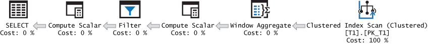
Observe how efficient the plan is, performing only one ordered scan of the index defined on col1. To apply the same technique to the temporal sequence, you simply use the DATEDIFF function to compute the difference between cur and nxt, and you use DATEADD to add or subtract an interval, like so:
WITH C AS
(
  SELECT col1 AS cur, LEAD(col1) OVER(ORDER BY col1) AS nxt
  FROM dbo.T2
)
SELECT DATEADD(day, 1, cur) AS rangestart, DATEADD(day, -1, nxt) rangeend
FROM C
WHERE DATEDIFF(day, cur, nxt) > 1;
Islands
The islands task involves identifying ranges of existing values. Here’s the desired output against the numeric sequence:
start_range end_range
----------- -----------
2           3
7           9
11          11
15          17
28          28
And here’s the desired output against the temporal sequence:
start_range end_range
----------- ----------
2019-02-02  2019-02-03
2019-02-07  2019-02-09
2019-02-11  2019-02-11
2019-02-15  2019-02-17
2019-02-28  2019-02-28
One of the most efficient solutions to the islands task involves using ranking calculations. You use the DENSE_RANK function to create a sequence of integers in col1 ordering, and you calculate the difference between col1 and the dense rank, like so:
SELECT col1,
  DENSE_RANK() OVER(ORDER BY col1) AS drnk,
  col1 - DENSE_RANK() OVER(ORDER BY col1) AS diff
FROM dbo.T1;

col1  drnk  diff
----- ----- -----
2     1     1
3     2     1
7     3     4
8     4     4
9     5     4
11    6     5
15    7     8
16    8     8
17    9     8
28    10    18
Observe that within an island the difference is the same, and that difference is unique for each island. That’s because within an island, both col1 and drnk keep advancing by the same interval. As soon as you jump to the next island, col1 increases by more than one interval, whereas drnk keeps increasing by one. Therefore, the difference in each island is greater than the previous island’s difference. Because this difference is the same within an island and unique for each island, you can use it as a group identifier. So, what’s left is just to group the rows by this difference and return the minimum and maximum col1 values in each group, like so:
WITH C AS
(
  SELECT col1, col1 - DENSE_RANK() OVER(ORDER BY col1) AS grp
  FROM dbo.T1
)
SELECT MIN(col1) AS start_range, MAX(col1) AS end_range
FROM C
GROUP BY grp;
The plan for this solution is shown in Figure 6-23.

The plan is very efficient because the computation of the dense rank value can rely on the ordering of the index on col1.
You might be wondering why we use the DENSE_RANK function and not ROW_NUMBER. This has to do with needing support for cases where the sequence values are not guaranteed to be unique. Using the ROW_NUMBER function, the technique works only when the sequence values are unique (which happens to be the case in our sample data), but it fails when duplicates are allowed. Using the DENSE_RANK function, the technique works both with unique and nonunique values; hence, I prefer to always use DENSE_RANK.
The technique can even work with temporal intervals, but it might not immediately be apparent how to adjust it for this case. Remember that the technique involves producing a group identifier—namely, a value that is the same for all members of the same island and different from the values produced for other islands. With the temporal sequence, the col1 values and dense rank values use different types of intervals—one uses an interval of 1 integer, and the other uses an interval of 1 day. To make the technique work, simply subtract from the col1 value as many times the temporal interval as the dense rank value. You need to use the DATEADD function to achieve this. Then you will get a date and time value as a result that is the same for all members of the same island and different from the values produced for other islands. Here’s the complete solution code:
WITH C AS
(
  SELECT col1, DATEADD(day, -1 * DENSE_RANK() OVER(ORDER BY col1), col1) AS grp
  FROM dbo.T2
)
SELECT MIN(col1) AS start_range, MAX(col1) AS end_range
FROM C
GROUP BY grp;
As you can see, instead of directly subtracting the result of the dense rank function from col1, you use DATEADD to subtract the dense rank multiplied by one day from col1.
There many examples of querying tasks where you need to use the islands technique, such as availability reports, periods of activity, and others. Earlier I demonstrated that you can even use the islands technique to handle interval packing.
There are versions of the islands task that are more complicated than the fundamental one. For example, say you are supposed to ignore gaps of up to a certain size—for example, in our date sequence, say you are supposed to ignore gaps of up to 2 days. Then the desired output would be the following:
rangestart rangeend
---------- ----------
2019-02-02 2019-02-03
2019-02-15 2019-02-17
2019-02-28 2019-02-28
2019-02-07 2019-02-11
Observe that the dates in February 2019 with the day units 7, 8, 9, and 11 are all part of one island starting with 7 and ending with 11. The gap between 9 and 11 is ignored because it isn’t greater than 2.
You can use the LAG and SUM window functions to handle this task. You first define a CTE called C1 based on a query against T2 computing an attribute called isstart. This attribute is a flag whose value is 0 when the current value isn’t the first in the island and 1 when it is. If the difference between the current col1 value and the previous value (obtained using the LAG function) is less than or equal to 2 days, the value is not the first value in the island; otherwise, it is the first value in the island.
Next, the code defines a CTE called C2 that computes a running total of the isstart flag, resulting in a unique value per island that you can use as a group identifier.
Finally, the outer query groups the rows from C2 by the island identifier and returns the minimum start time and maximum end time as the island boundaries.
Here’s the complete solution code:
WITH C1 AS
(
  SELECT col1,
    CASE
      WHEN DATEDIFF(day, LAG(col1) OVER(ORDER BY col1), col1) <= 2
        THEN 0
      ELSE 1
    END AS isstart
  FROM dbo.T2
),
C2 AS
(
  SELECT *,
    SUM(isstart) OVER(ORDER BY col1 ROWS UNBOUNDED PRECEDING) AS grp
  FROM C1
)
SELECT MIN(col1) AS rangestart, MAX(col1) AS rangeend
FROM C2
GROUP BY grp;
The execution plan for this query is shown in Figure 6-24.

This plan is highly efficient, applying one ordered scan of the data, and avoiding the need for sorting altogether.
This technique where you create a flag that tells you whether the current event starts a new island after obtaining data from the previous row using LAG, and then apply a running total calculation to produce an island identifier, is very powerful. It can be used to solve almost any kind of islands task that you can think about.
Here’s another example. Use the following code to generate a new table called T1 and fill it with sample data:
DROP TABLE IF EXISTS dbo.T1;

CREATE TABLE dbo.T1
(
  id  INT         NOT NULL PRIMARY KEY,
  val VARCHAR(10) NOT NULL
);
GO

INSERT INTO dbo.T1(id, val) VALUES
  (2, 'a'),
  (3, 'a'),
  (5, 'a'),
  (7, 'b'),
  (11, 'b'),
  (13, 'a'),
  (17, 'a'),
  (19, 'a'),
  (23, 'c'),
  (29, 'c'),
  (31, 'a'),
  (37, 'a'),
  (41, 'a'),
  (43, 'a'),
  (47, 'c'),
  (53, 'c'),
  (59, 'c');
The task in this case is to identify consecutive ranges of IDs where the value in the val attribute remains the same. Observe that there can be multiple islands associated with the same value in val. Here’s the desired output for the given sample data:
rangestart  rangeend    val
----------- ----------- ----------
2           5           a
7           11          b
13          19          a
23          29          c
31          43          a
47          59          c
Here’s the solution that applies our flexible technique to handle this task:
WITH C1 AS
(
  SELECT id, val, CASE WHEN val = LAG(val) OVER(ORDER BY id) THEN 0 ELSE 1 END     AS isstart
  FROM dbo.T1
),
C2 AS
(
  SELECT *,
    SUM(isstart) OVER(ORDER BY id ROWS UNBOUNDED PRECEDING) AS grp
  FROM C1
)
SELECT MIN(id) AS rangestart, MAX(id) AS rangeend, val
FROM C2
GROUP BY grp, val;
The query in the CTE called C1 computes the isstart flag, setting it to 0 when the value in the current and previous rows are the same, otherwise to 1. The query in the CTE called C2 computes a running total of the isstart flag, resulting in an island, or group, identifier called grp. The outer query then groups the rows from C2 by grp and val and returns the minimum ID and maximum ID as the island boundaries.
Gaps and islands tasks can also be solved very elegantly using row pattern recognition. Make sure that you check out Chapter 4 to see how.
Median
In Chapters 2 and 3, I discussed how to compute percentiles. I mentioned that the 50th percentile—commonly known as the median—represents, loosely speaking, the value in the population that 50 percent of the values are less than. I provided solutions to calculating any percentile. Here, I’ll just remind you of the solution using the PERCENTILE_CONT function (CONT for the continuous distribution model) and then, for the sake of the exercise, show additional interesting solutions specific to the median calculation without using the built-in function.
For sample data, I’ll use the Stats.Scores table, which holds student test scores. Suppose your task was to compute, for each test, the median score assuming continuous distribution model. If there’s an odd number of student test scores for a given test, you’re supposed to return the middle score. If there’s an even number, you’re supposed to return the average of the two middle scores. Here’s the desired output for the given sample data:
testid     median
---------- -------
Test ABC   75
Test XYZ   77.5
As already mentioned in this book, the function PERCENTILE_CONT is used to compute percentiles assuming a continuous distribution model. However, this function wasn’t implemented as a grouped ordered set function; rather, it was implemented as a window function. This means that you can use it to return a percentile along with all detail rows but to return it only once per group, you need to add a DISTINCT clause, like so:
SELECT DISTINCT testid,
  PERCENTILE_CONT(0.5) WITHIN GROUP(ORDER BY score) OVER(PARTITION BY testid) AS median
FROM Stats.Scores;
It’s a little bit awkward, but it works.
As an exercise, to compute median without the built-in PERCENTILE_CONT function, you have to be more creative. One solution is to compute, for each row, a position within the test based on score ordering (call it pos) and the count of scores in the respective test (call it cnt). To compute pos, you use the ROW_NUMBER function, and to compute cnt, you use the COUNT window aggregate function. Then you filter only the rows that are supposed to participate in the median calculation—namely, the rows where pos is either equal to (cnt + 1) / 2 or (cnt + 2) / 2. Note that the expressions use integer division, so any fraction is truncated. When there is an odd number of elements, both expressions return the same middle point. For example, when there are 9 elements in the group, both expressions return 5. When there is an even number of elements, the expressions return the two middle points. For example, when there are 10 elements in the group, the expressions return 5 and 6. After you filter the right rows, what’s left is to group the rows by the test ID and return for each test the average score. Here’s the complete solution query:
WITH C AS
(
  SELECT testid, score,
    ROW_NUMBER() OVER(PARTITION BY testid ORDER BY score) AS pos,
    COUNT(*) OVER(PARTITION BY testid) AS cnt
  FROM Stats.Scores
)
SELECT testid, AVG(1. * score) AS median
FROM C
WHERE pos IN( (cnt + 1) / 2, (cnt + 2) / 2 )
GROUP BY testid;
Another interesting solution involves computing two row numbers—one in ascending score, studentid ordering (studentid added for determinism), and another in descending ordering. Here’s the code to compute the two row numbers followed by its output:
SELECT testid, score,
  ROW_NUMBER() OVER(PARTITION BY testid ORDER BY score, studentid) AS rna,
  ROW_NUMBER() OVER(PARTITION BY testid ORDER BY score DESC, studentid DESC)     AS rnd
FROM Stats.Scores;

testid     score rna  rnd
---------- ----- ---- ----
Test ABC   95    9    1
Test ABC   95    8    2
Test ABC   80    7    3
Test ABC   80    6    4
Test ABC   75    5    5
Test ABC   65    4    6
Test ABC   55    3    7
Test ABC   55    2    8
Test ABC   50    1    9
Test XYZ   95    10   1
Test XYZ   95    9    2
Test XYZ   95    8    3
Test XYZ   80    7    4
Test XYZ   80    6    5
Test XYZ   75    5    6
Test XYZ   65    4    7
Test XYZ   55    3    8
Test XYZ   55    2    9
Test XYZ   50    1    10
Can you generalize a rule that identifies the rows that need to participate in the median calculation?
Observe that when there’s an odd number of elements, the median is where the two row numbers are the same. When there’s an even number of elements, the median elements are where the absolute difference between the two row numbers is equal to 1. To merge the two rules, the median elements are in the rows where the absolute difference between the two row numbers is less than or equal to 1. Here’s the complete solution code that relies on this rule:
WITH C AS
(
  SELECT testid, score,
    ROW_NUMBER() OVER(PARTITION BY testid ORDER BY score, studentid) AS rna,
    ROW_NUMBER() OVER(PARTITION BY testid ORDER BY score DESC, studentid DESC)
       AS rnd
  FROM Stats.Scores
)
SELECT testid, AVG(1. * score) AS median
FROM C
WHERE ABS(rna - rnd) <= 1
GROUP BY testid;
The last two solutions perform quite well when the group element (the test ID in our case) has low density. When it has high density, a different solution tends to be more optimal. It’s a solution that uses a combination of the APPLY operator and OFFSET-FETCH filter.
The idea is to handle each group separately. You use one query to identify the groups with their relevant parameters and another to handle each group. The first query is a grouped query that based on the count of test scores per test ID computes parameters for an OFFSET-FETCH filter. The second query is an applied correlated query that skips and filters the right number of test scores for the current test ID. You use the following formulas to compute the offset value (call it ov) and fetch value (call it fv) columns:
■ ov = (COUNT(*) - 1) / 2
■ fv = 2 - COUNT(*) % 2
The calculation of ov uses integer division since the count is an integer. The % sign is used as a modulo operator; it tells you whether the count is odd or even.
Once you have your grouped query compute the ov and fv columns, you define a CTE named C based on it and have the outer query against C use CROSS APPLY to apply an OFFSET-FETCH query that skips and fetches the right number of rows, group the result by testid, and compute the average of the returned scores.
Here’s the complete solution query:
WITH C AS
(
  SELECT testid, (COUNT(*) - 1) / 2 AS ov, 2 - COUNT(*) % 2 AS fv
  FROM Stats.Scores
  GROUP BY testid
)
SELECT C.testid, AVG(1. * A.score) AS median
FROM C CROSS APPLY ( SELECT S.score
                     FROM Stats.Scores AS S
                     WHERE S.testid = C.testid
                     ORDER BY S.score
                     OFFSET C.ov ROWS FETCH NEXT C.fv ROWS ONLY ) AS A
GROUP BY C.testid;
You do want to make sure that you have an index on the key list (testid, score) to support all of the presented solutions.
Conditional Aggregate
Our next task involves computing a running total that always returns a non-negative value. That is, if the running total is negative at a point, return zero instead. Then, when you move to the next item in the sequence, you proceed from 0. The practical use case is processing transactions that consume quantities from some stock, and when the stock level drops below zero, you replenish the stock from elsewhere. For sample data, use the following code, which creates and populates a table called T1:
USE TSQLV5;

DROP TABLE IF EXISTS dbo.T1;
GO

CREATE TABLE dbo.T1
(
  ordcol  INT NOT NULL PRIMARY KEY,
  datacol INT NOT NULL
);

INSERT INTO dbo.T1 VALUES
  (1,   10),
  (4,  -15),
  (5,    5),
  (6,  -10),
  (8,  -15),
  (10,  20),
  (17,  10),
  (18, -10),
  (20, -30),
  (31,  20);
According to the description of the task, here’s the desired output for the given sample data, computing a non-negative sum of datacol (representing the quantity of the transaction) based on ordcol ordering (representing chronological order):
ordcol      datacol     nonnegativesum replenish
----------- ----------- -------------- -----------
1           10          10             0
4           -15         0              5
5           5           5              0
6           -10         0              5
8           -15         0              15
10          20          20             0
17          10          30             0
18          -10         20             0
20          -30         0              10
31          20          20             0
I’ll present an elegant solution that uses window functions. Listing 6-17 shows the complete solution code, followed by its output (adding the intermediate computations partsum and adjust to help explain the solution):
LISTING 6-17 Solution for Nonnegative Running Sum Task
WITH C1 AS
(
  SELECT ordcol, datacol,
    SUM(datacol) OVER (ORDER BY ordcol
                       ROWS UNBOUNDED PRECEDING) AS partsum
  FROM dbo.T1
),
C2 AS
(
  SELECT *,
    MIN(partsum) OVER (ORDER BY ordcol
                       ROWS UNBOUNDED PRECEDING) as mn
  FROM C1
)
SELECT ordcol, datacol, partsum, adjust,
  partsum + adjust AS nonnegativesum,
  adjust - LAG(adjust, 1, 0) OVER(ORDER BY ordcol) AS replenish
FROM C2
  CROSS APPLY(VALUES(CASE WHEN mn < 0 THEN -mn ELSE 0 END)) AS A(adjust);

ordcol  datacol  partsum  adjust  nonnegativesum replenish
------- -------- -------- ------- -------------- ----------
1       10       10       0       10             0
4       -15      -5       5       0              5
5       5        0        5       5              0
6       -10      -10      10      0              5
8       -15      -25      25      0              15
10      20       -5       25      20             0
17      10       5        25      30             0
18      -10      -5       25      20             0
20      -30      -35      35      0              10
31      20       -15      35      20             0
The code defining the CTE called C1 creates an attribute called partsum that computes a plain running total of datacol based on ordcol ordering. This partsum attribute can be negative because the values in datacol can be negative. Then the code defining the CTE called C2 queries C1, creating an attribute called adjust that is the additive inverse of the minimum partsum value when negative up to the current point. The outer query then computes the nonnegative sum by adding adjust to partsum, and the replenish quantity by subtracting the adjust value of the previous row, if present, from the current row’s adjust value.
It can take a few rounds of going over this output to see that the logic works, but it does!
Note This and similar capped sum tasks can be handled very easily and elegantly using row pattern recognition. Make sure to check such solutions in Chapter 4.
Sorting Hierarchies
Suppose that you need to present information from some hierarchy in a sorted fashion. You’re supposed to present a parent before its descendants. Also, you need to be able to control the order among siblings. For sample data, use the code in Listing 6-18, which creates and populates a table called dbo.Employees. (This is not to be confused with the existing HR.Employees table that has different data.)
LISTING 6-18 Code to Create and Populate the Employees Table
USE TSQLV5;

DROP TABLE IF EXISTS dbo.Employees;
GO
CREATE TABLE dbo.Employees
(
  empid   INT         NOT NULL
    CONSTRAINT PK_Employees PRIMARY KEY,
  mgrid   INT         NULL
    CONSTRAINT FK_Employees_mgr_emp REFERENCES dbo.Employees,
  empname VARCHAR(25) NOT NULL,
  salary  MONEY       NOT NULL,
  CHECK (empid <> mgrid)
);

INSERT INTO dbo.Employees(empid, mgrid, empname, salary) VALUES
  (1,  NULL, 'David'  , $10000.00),
  (2,  1,    'Eitan'  ,  $7000.00),
  (3,  1,    'Ina'    ,  $7500.00),
  (4,  2,    'Seraph' ,  $5000.00),
  (5,  2,    'Jiru'   ,  $5500.00),
  (6,  2,    'Steve'  ,  $4500.00),
  (7,  3,    'Aaron'  ,  $5000.00),
  (8,  5,    'Lilach' ,  $3500.00),
  (9,  7,    'Rita'   ,  $3000.00),
  (10, 5,    'Sean'   ,  $3000.00),
  (11, 7,    'Gabriel',  $3000.00),
  (12, 9,    'Emilia' ,  $2000.00),
  (13, 9,    'Michael',  $2000.00),
  (14, 9,    'Didi'   ,  $1500.00);

CREATE UNIQUE INDEX idx_unc_mgrid_empid ON dbo.Employees(mgrid, empid);
Suppose that you need to present employees in hierarchical order—always presenting the manager before subordinates—and sorting siblings by empname. To achieve this task, you can use two main tools: the ROW_NUMBER function and a recursive CTE. You define a regular CTE called EmpsRN first, where you compute an attribute called n representing a row number partitioned by mgrid and ordered by empname, empid (empid added for determinism):
WITH EmpsRN AS
(
  SELECT *,
    ROW_NUMBER() OVER(PARTITION BY mgrid ORDER BY empname, empid) AS n
  FROM dbo.Employees
)
SELECT * FROM EmpsRN;

empid  mgrid  empname  salary    n
------ ------ -------- --------- ---
1      NULL   David    10000.00  1
2      1      Eitan    7000.00   1
3      1      Ina      7500.00   2
5      2      Jiru     5500.00   1
4      2      Seraph   5000.00   2
6      2      Steve    4500.00   3
7      3      Aaron    5000.00   1
8      5      Lilach   3500.00   1
10     5      Sean     3000.00   2
11     7      Gabriel  3000.00   1
9      7      Rita     3000.00   2
14     9      Didi     1500.00   1
12     9      Emilia   2000.00   2
13     9      Michael  2000.00   3
Next, you define a recursive CTE called EmpsPath, where you iterate through the employees one level at a time, starting with the root (CEO), then to direct subordinates, then to subordinates of subordinates, and so on. You construct a binary path for each employee that starts as an empty path for the root, and in each level of subordinates, you concatenate the manager’s path with the binary form of n (the row number). Note that to minimize the size of the path, you need only enough bytes to cover the maximum number of direct subordinates a single manager can have. For example, a single byte is sufficient for up to 255 direct subordinates, two bytes are sufficient for up to 32,767 direct subordinates, and so on. Let’s assume that we need two bytes in our case. You can also compute the level of the employee in the tree (the distance from the root) by assigning the level 0 to the root, and for a subordinate, you add 1 to the manager’s level. Listing 6-19 shows the code that computes both the sort path (sortpath) and the level (lvl).
LISTING 6-19 Code Computing sortpath and lvl
WITH EmpsRN AS
(
  SELECT *,
    ROW_NUMBER() OVER(PARTITION BY mgrid ORDER BY empname, empid) AS n
  FROM dbo.Employees
),
EmpsPath
AS
(
  SELECT empid, empname, salary, 0 AS lvl,
    CAST(0x AS VARBINARY(MAX)) AS sortpath
  FROM dbo.Employees
  WHERE mgrid IS NULL

  UNION ALL

  SELECT C.empid, C.empname, C.salary, P.lvl + 1,
    P.sortpath + CAST(n AS BINARY(2)) AS sortpath
  FROM EmpsPath AS P
    INNER JOIN EmpsRN AS C
      ON C.mgrid = P.empid
)
SELECT *
FROM EmpsPath;

empid  empname  salary    lvl  sortpath
------ -------- --------- ---- -------------------
1      David    10000.00  0    0x
2      Eitan    7000.00   1    0x0001
3      Ina      7500.00   1    0x0002
7      Aaron    5000.00   2    0x00020001
11     Gabriel  3000.00   3    0x000200010001
9      Rita     3000.00   3    0x000200010002
14     Didi     1500.00   4    0x0002000100020001
12     Emilia   2000.00   4    0x0002000100020002
13     Michael  2000.00   4    0x0002000100020003
5      Jiru     5500.00   2    0x00010001
4      Seraph   5000.00   2    0x00010002
6      Steve    4500.00   2    0x00010003
8      Lilach   3500.00   3    0x000100010001
10     Sean     3000.00   3    0x000100010002
What’s left to do to guarantee that the employees are presented in the desired order is to order the rows by sortpath. You can also achieve indentation in the output based on the employee’s level in the hierarchy by replicating a string lvl times. Listing 6-20 provides the complete solution code.
LISTING 6-20 Sorting Employee Hierarchy with Siblings Sorted by empname
WITH EmpsRN AS
(
  SELECT *,
    ROW_NUMBER() OVER(PARTITION BY mgrid ORDER BY empname, empid) AS n
  FROM dbo.Employees
),
EmpsPath
AS
(
  SELECT empid, empname, salary, 0 AS lvl,
    CAST(0x AS VARBINARY(MAX)) AS sortpath
  FROM dbo.Employees
  WHERE mgrid IS NULL

  UNION ALL

  SELECT C.empid, C.empname, C.salary, P.lvl + 1,
    P.sortpath + CAST(n AS BINARY(2)) AS sortpath
  FROM EmpsPath AS P
    INNER JOIN EmpsRN AS C
      ON C.mgrid = P.empid
)
SELECT empid, salary, REPLICATE(' | ', lvl) + empname AS empname
FROM EmpsPath
ORDER BY sortpath;
Observe in the output of this solution that a manager always appears before his or her subordinates, and that siblings are sorted by empname:
empid       salary                empname
----------- --------------------- --------------------
1           10000.00                David
2           7000.00                | Eitan
5           5500.00                |  | Jiru
8           3500.00                |  |  | Lilach
10          3000.00                |  |  | Sean
4           5000.00                |  | Seraph
6           4500.00                |  | Steve
3           7500.00                | Ina
7           5000.00                |  | Aaron
11          3000.00                |  |  | Gabriel
9           3000.00                |  |  | Rita
14          1500.00                |  |  |  | Didi
12          2000.00                |  |  |  | Emilia
13          2000.00                |  |  |  | Michael
If you need siblings to be sorted differently—say, by salary—simply change the ROW_NUMBER function’s window ordering clause, accordingly, as shown in Listing 6-21.
LISTING 6-21 Sorting Employee Hierarchy with Siblings Sorted by salary
WITH EmpsRN AS
(
  SELECT *,
    ROW_NUMBER() OVER(PARTITION BY mgrid ORDER BY salary, empid) AS n
  FROM dbo.Employees
),
EmpsPath
AS
(
  SELECT empid, empname, salary, 0 AS lvl,
    CAST(0x AS VARBINARY(MAX)) AS sortpath
  FROM dbo.Employees
  WHERE mgrid IS NULL
  UNION ALL
  SELECT C.empid, C.empname, C.salary, P.lvl + 1,
    P.sortpath + CAST(n AS BINARY(2)) AS sortpath
  FROM EmpsPath AS P
    INNER JOIN EmpsRN AS C
      ON C.mgrid = P.empid
)
SELECT empid, salary, REPLICATE(' | ', lvl) + empname AS empname
FROM EmpsPath
ORDER BY sortpath;
Here’s the output of this query:
empid       salary                empname
----------- --------------------- --------------------
1           10000.00                David
2           7000.00                | Eitan
6           4500.00                |  | Steve
4           5000.00                |  | Seraph
5           5500.00                |  | Jiru
10          3000.00                |  |  | Sean
8           3500.00                |  |  | Lilach
3           7500.00                | Ina
7           5000.00                |  | Aaron
9           3000.00                |  |  | Rita
14          1500.00                |  |  |  | Didi
12          2000.00                |  |  |  | Emilia
13          2000.00                |  |  |  | Michael
11          3000.00                |  |  | Gabriel
Summary
I can’t keep myself from admiring the beautiful design of window functions. They’re engineered to overcome a number of shortcomings of more traditional SQL constructs, and they lend themselves to excellent optimization. You saw in this book that there are so many querying tasks that can be handled both elegantly and efficiently with window functions. I hope you will think of what you saw as just the start, and that you will find interesting and creative ways of your own to use them.
Standard SQL sees the great value in window functions and therefore, keeps adding more and more functions and functionality. Let’s hope we see more powerful analytical capabilities added to SQL Server in the future, such as row-pattern recognition and additional windowing support.