
Chapter 5
The Analysis of Bivariate Data—Diagnostics
Diagnosing Linearity: Transformations
Introduction
We saw in chapter 4 that JMP is a terrific partner to have when performing regression diagnosis. We breezed through a regression analysis of the gastric emptying time data with ease, generally checking the assumptions for the straight-line model with gratifying results. The data turned out to be decently well behaved, so we could safely operate under the presumption of meeting the assumptions. However, not all data will be benignly distributed, and in this chapter I will demonstrate some of the capabilities of JMP in the context of less well-behaved data than we have previously presented. The skeptical but judicious consideration of the plausibility of the regression assumptions and careful search for troublesome points generally is termed “model adequacy checking” and “diagnosis” of a fitted line (Montgomery, Peck, and Vining, 2006).
Weisberg (1983) refers to diagnostics as model criticism and uses the term to refer to statistics rather than graphics. He also separates diagnostics from influence analysis, his term for a critical focus on individual points. Here I will generally use the term diagnosis to mean verifying and checking assumptions associated with fitting a straight line to data. The mathematical statistics underlying model checking is beyond the level of elementary statistics. Montgomery, Peck, and Vining (2006) and Kutner et al. (2005) provide excellent detailed presentations. Fortunately, we can use relatively elementary graphic and numerical diagnostic methods with simple “straight-line” regression. In this chapter we focus on useful JMP techniques applicable to demonstrably nonlinear data.
The analysis of individual points will involve examination of residuals, outliers, and influential points. Simple definitions of outlier and influential are elusive, and in elementary statistics the identification of outliers and influential points involves a significant amount of subjective judgment, as opposed to strict numerical calculations according to an agreed-upon standard. In the subsequent discussion I will generally follow Montgomery, Peck, and Vining (2006): “Outliers are data points that are not typical of the rest of the data.” Hawkins (1980) also captures this idea: “An outlier is an observation that deviates so much from other observations as to arouse suspicion that it was generated by a different mechanism.” Montgomery, Peck, and Vining (2006) declare a point influential if “it has a noticeable impact on the model coefficients in that it ‘pulls’ the regression model in its direction.”
Outliers
Outliers are data values that appear to be inconsistent with the general trend of our data. Outliers are problematic because they can arise for any of several reasons, and it may be impossible to identify which of these has produced a particular outlier. One possibility is that outlying values are the result of natural variability in the variable(s) under study; that is, the outliers are not actually inconsistent at all. Variability happens.
A crucially important assumption in any statistical analysis is that variables under study are normally distributed. If the variable is in reality heavy-tailed or skewed, data values that would appear to be outliers under an assumption of normality could instead be perfectly reasonable observations. A second possibility is that an error has occurred in the data collection process, perhaps due to a flawed physical measuring device or human error in recording the data. In some cases it may be possible to determine that an error is a recording error, perhaps a misplaced decimal or a digit reversal at data entry. If data entry records have been judiciously kept, such an error may be corrected by reviewing the data entry process.
Unfortunately, while statistics can be created that may nominate points to be outliers, the statistics alone cannot decide the issue. Identifying a value as a potential outlier and subsequently deciding on a proper course of action (deleting the data value, modifying the value, noting the value in a footnote) is a human decision-making activity, fraught with subjectivity. The best that may be hoped is that the decision will be successfully guided by the data analyst’s knowledge, wisdom, and experience.
In a bivariate setting, points can be outliers for perhaps two reasons: (a) they have an unusual x and/or y value, or (b) they have unusual residuals when a regression analysis is performed. As an example, we will consider the data in the JMP file UnusualBears. These data are measurements on twelve female black bears (Ursus americanus) from a study by Brodeur et al. (2008). The investigators were interested in the behavior of these bears in Canadian forests. Over the past thirty years increased logging has pushed these creatures northward into less favorable habitat, and they are now confined to an area equal to approximately 60 percent of their historical range. The more northern forests offer colder winters and shorter growing seasons, a situation that would be expected to influence the bears' ecology.
The bears in this study were snared and weighed, their ages estimated, their necks radio-collared, and their ears fitted with tags for identification. (One can only imagine what their mates thought of all this.) Over the course of three years, the researchers gathered information about the bears' home ranges. The home range of an animal—the typical area over which it travels—is generally a function of the quality of food in the area. If the food is scarce, a larger area must be searched for food. It is this search behavior that was of interest to the researchers. The home range data are given for two time periods: summer/fall and spring.
Three scatterplots from the data are shown below in figure 5.1.
Figure 5.1 Outliers
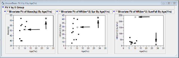
To follow along in JMP for practice, here are the steps to produce the plots using the original file data:
1. Select Analyze → Fit Y by X → Age(Yrs) → X, Factor.
2. Select Mass(kg), HR(km^2) Spr, and HR(km^2) SumFall for the Y, Response.
3. Click OK.
4. For all three scatterplots change the Age (Yrs) scale to run from 0 to 35.
5. For the Mass(kg) By Age (Yrs) plot, change the Mass(kg) scale to run from 35 to 65, with increments of 5 and 1 tick mark.
6. Click and drag in the row column to darken the markers in the plots.
7. Use the Tools → Line feature to add arrows near Bear #5 and Bear #7.
8. Right click on the lines and choose PointTo to change the line segments to arrows.
9. Right click on the arrows and choose your favorite colors from the drop-down box.
Note that one could add text boxes to identify the bears of interest; here I chose to highlight the marker capability of JMP. Inspection of the plots reveals that Bear #5 (the square in the plot) is older than the rest (a possible “age outlier”), but she is not particularly different in either mass or home range. Bear #7 (the open circle) is rather pedestrian in age, mass, and spring home range, but she has a large summer/fall home range (a possible “home range” outlier). Inspection of the stem and leaf plots in figure 5.2 will give you a good idea of how far these bears' errant values of age and summer/fall home range fall from their colleagues.
Figure 5.2 Age ranges
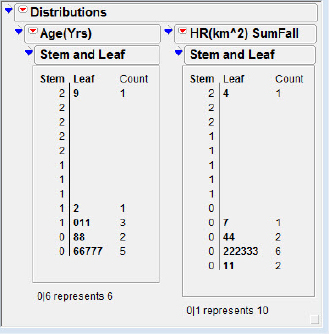
The typical longevity of these creatures is known to be twenty to thirty-five years, so Bear #5 is clearly getting long in the tooth. However, the statistically outlying summer/fall home range of Bear #7 is more difficult to assess. Is Bear #7 a very special bear, or is the outlier attempting to signal that more bears are out there with very large summer/fall home ranges? The researchers did not mention any malfunction of their measuring devices, so that does not appear to be the reason for the large home range. We (and the researchers) are left with two possible explanations for the outliers: They may be unlikely but possible chance occurrences, or they may be signals that older and/or more wide-ranging bears are out there in the northern forests. The statistics and graphs cannot tell us which, if either, answer is correct.
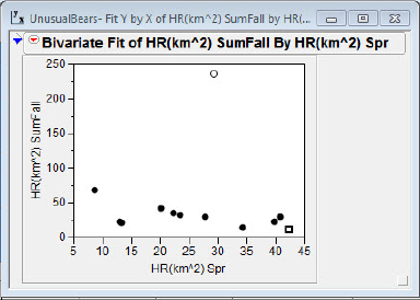
When we perform a regression analysis it is, of course, possible to have outliers in the sense discussed earlier. In addition, once a straight line is fitted to data we may be presented with an additional sort of outlier: points with unusually large residuals. Figure 5.3(a) shows a scatterplot of the home ranges of summer/fall versus spring. Our friend Bear #7 sticks out like a sore paw from the rest of the data. Bear #5 is at the upper end of the spring home range but is otherwise not distinguished in this plot.
Figure 5.3(a) Large residual?
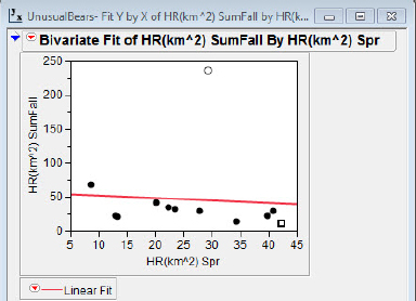
It will come as no surprise that when a line is fit to these data, Bear #7 has a very large residual, as seen in figure 5.3(b). Thus, Bear #7 is an outlier in both senses: well away from the herd and possesses a large residual when a line is fit to the data.
Figure 5.3(b) Large residual!
Just how far Bear #7 deviates from the predicted value can be seen with a stem and leaf plot of the residuals as presented in figure 5.4. Recall that JMP will save the residuals in a separate column.
Figure 5.4 HR residuals
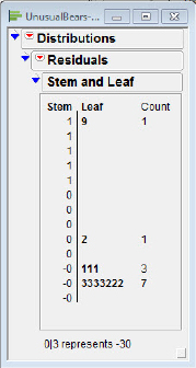
1. Select Linear Fit → Save residuals.
We can direct JMP to construct a stem and leaf plot of the residuals using this sequence:
2. Select Analyze → Distribution.
Residuals can be standardized in the usual way by subtracting the mean residual (0.0) and dividing by the standard deviation (root mean square error, displayed in the Summary of Fit in JMP):
![]()
The residuals so standardized have a mean of 0.0 and a standard deviation approximately equal to 1.0; a “large” standardized residual potentially indicates an outlier. To standardize all the residuals, create a new column (StandResids in my case). After clicking on the top of the newly created StandResids column, key in:
3. Select Column Properties → Formula → Edit Formula.
We also did this in chapter 3. Then provide the formula as shown in figure 5.5(a). The ordinary and resulting standardized residuals are shown in figure 5.5(b).
Figure 5.5(a) Standardizing the residuals
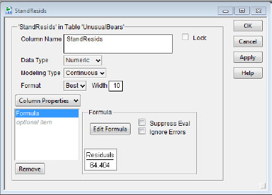
Figure 5.5(b) Comparison
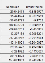
The reader will note that I have chosen to demonstrate calculating the standardized residuals with JMP because this standardization process is well known in elementary statistics. Other more advanced methods for scaling residuals exist and are readily available in JMP. Consult Montgomery, Peck, and Vining (2006) for an in-depth discussion of scaling residuals, as well as the Analyze → Fit Model sequence in JMP for execution.
I will conclude this discussion of outliers with a teaching observation. My classroom presentation of outliers frequently leads to extended discussions that can be time consuming. As we know, class time is a valuable commodity. Does classroom discussion of outliers possess a sufficiently counterbalancing value add? I believe it does, for two reasons. First, when students go on to analyze data “for real,” outliers will appear; their statistics course should prepare them for this eventuality. Second, there is a significant amount of judgment involved in handling outliers; classroom discussion helps cement the notion that differing points of view should be allowed, respected, considered, and debated.
Influential Points
In regression analysis the values of the explanatory variable play a more important role than the values of the response variable. Each of the points has equal weight in determining the intercept of the best-fit line, but the slope is more influenced by values of x that are far removed from ![]() . Points with unusually low or high x values are said to have high “leverage.” Archimedes (287–212 BCE) was quoted as saying, “Give me a lever long enough and a fulcrum on which to place it, and I shall move the world.” A modern-day statistician might similarly suggest that given a point with a sufficiently large x-coordinate, he or she could move the slope of the best-fit line. A high-leverage point is not, however, completely sufficient to change the regression world; the power of a single point to change the slope depends not only on the x-value, but also on the y-value of the point in question.
. Points with unusually low or high x values are said to have high “leverage.” Archimedes (287–212 BCE) was quoted as saying, “Give me a lever long enough and a fulcrum on which to place it, and I shall move the world.” A modern-day statistician might similarly suggest that given a point with a sufficiently large x-coordinate, he or she could move the slope of the best-fit line. A high-leverage point is not, however, completely sufficient to change the regression world; the power of a single point to change the slope depends not only on the x-value, but also on the y-value of the point in question.
As an example, we consider data from Jeanne and Nordheim (1996). These investigators studied the behavior of Polybia occidentalis, a social wasp found in Costa Rica. These data are found in the JMP file UnusualWasps. Jeanne and Nordheim were interested in the forces that determine the swarm size of these social insects, in particular the relationship between swarm size and productivity of the workers. After marking a few adults for future identification, they dismantled their existing nests, forcing active colonies to desert their locations and build new nests. The newly formed nests were left undisturbed for twenty-five days, at which time the researchers collected the individuals from each new colony. They measured different characteristics of the nests, including numbers of queens and workers, and various weights. During nest development, this species of wasp initially has a high number of queens, a number that is eventually reduced to a few or to one. The researchers used weights of the brood and nest as measures of the amount of work performed during new nest construction.
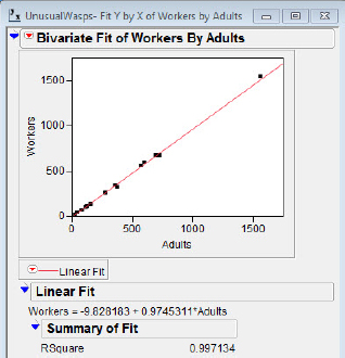
In figures 5.6(a) and 5.6(b) the results of two regressions on number of workers versus number of adults are shown. In figure 5.6(a) the point (1562, 1547) is included in the regression, but in figure 5.6(b) the point is excluded from the regression fit but is plotted. I should note in passing that the incredibly good fit (r2 = 0.999) results from the nature of the variables more than anything else. The adults in a nest consist of queens and workers, and there are many more workers than queens. The target of our focus with these data is the notion that while the point at (1562, 1547) is a point with high leverage (since its x value is unusual), it has little influence on the regression statistics because of its placement very near the regression line.
Figure 5.6(a) Point included
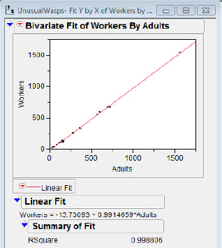
Figure 5.6(b) Point excluded
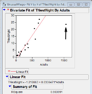
In figures 5.6(c) and 5.6(d) the results of two regressions on the total nest weight versus number of adults are shown. With these data we note that the point at (1562, 23.49) is a point with high leverage (its x value is unusually large in this data set), and in addition it has great influence on the regression statistics. The estimate of the slope increases by 68 percent, and r2 by 24 percent, when the point is deleted. The point is deleted from the analysis but is still plotted by JMP.
Figure 5.6(c) Point included
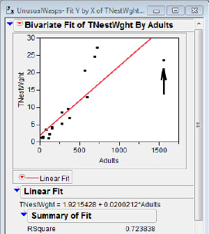
Figure 5.6(d) Point excluded
Before moving on to address transformations of data, I will reiterate that it is not a desirable situation if the straight-line model coefficients and/or other properties are greatly affected by a single point or a small group of points. If the influential points are “bad” points, the result of a mis-measure or a nest not representative of the population, they should be corrected or eliminated. On the other hand, if they actually are “good” points the model may have to be re-evaluated.
Diagnosing Linearity: Transformations
It sometimes happens that linear regression is plagued not by isolated outliers or influential points, but by whole sets of points that refuse to array themselves in a straight line. This can happen for a variety of reasons, the most common one being that the relation between two variables is not quite as straightforward as we might initially believe. In some elementary cases of bivariate analysis we can use linear regression in the face of a more complicated relation using the technique of transformation of variables. In elementary statistics, the “logarithmic” transformation is quite commonly used. The logarithmic transformation involves replacing the value of a variable, x, with a “transformed” variable, log(x) or ln(x), in the regression analysis. Three regression situations where log transformations turn out to be helpful include:
![]() y is reasonably modeled by a logarithmic function of x: y = α + β ln(x)
y is reasonably modeled by a logarithmic function of x: y = α + β ln(x)
![]() y is reasonably modeled by an exponential function of x: y = αeβx
y is reasonably modeled by an exponential function of x: y = αeβx
![]() y is reasonably modeled by a “power” function of x: y = αxβ
y is reasonably modeled by a “power” function of x: y = αxβ
To illustrate how JMP generally handles transformations we will specifically consider data from each of these situations.
The Log Model: y = α + βln(x)
Opfer and Siegler (2007) reported on an aspect of the development of the numerical estimation skills of children, ages 5 to 10 years. Educators believe that estimation skills are important in the development of mathematical capabilities (NCTM, 1980, 1989, 2000). Numerical estimation involves estimating distance, amount of money, counts of discrete objects—and the locations of numbers on number lines. Studies have indicated that individuals appear to become skillful at different types of these estimation tasks at about the same age, leading to speculation that numerical estimation is a single category of cognitive development. An example of the estimation task presented to the children by Opfer and Siegler is shown in figure 5.7.
Figure 5.7 The estimation task (slightly modified from the original)
![]()
In the interval above, with 0 and 1000 as endpoints, where would you put 35?
The children were given a set of these numbers and asked to put a mark on the number line that would correspond to the given numbers. The investigators found that as children develop, numerical magnitudes appear to be initially represented logarithmically. In other words, children tend to represent the difference between $1 and $100 as larger than the difference between $901 and $1000. We note here that this actually does make a certain amount of sense—the difference between two and three pieces of chocolate (a 50 percent increase) might seem a lot greater than the difference between ninety-two and ninety-three pieces (a 1 percent increase). Perhaps this logarithmic estimation is firm-wired into our brains at birth and replaced by a more realistic understanding with experience. In any case, chocolate-satisfied or not, children gradually “grow into” a linear representation.
We will use the researchers' data for second graders (Opfer, n.d.) to illustrate a couple of JMP capabilities: (a) fitting nonlinear regression functions, and (b) displaying more than one model fit to data on a single plot. The data are in the JMP file NumberLine.
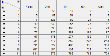
The initial data should appear as shown in figure 5.8. As explained in chapter 4, I have changed the markers to be large dots in order to make them easier to see in the plots. The Actual column contains the true location of the numbers on the number line. The 2nd column contains the median value for Opfer and Siegler’s second-grade subjects' responses to the “Actual” numbers being presented.
Figure 5.8 Opfer’s data
1. Select Analyze → Fit Y by X.
2. Select Actual → X, Factor.
3. Select 2nd > Y, Response.
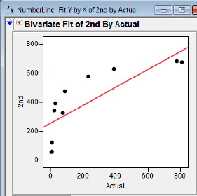
The first hint of difficulty when analyzing bivariate data usually appears when we try to fit the straight line to the data. The result of this initial fit is shown in figure 5.9. The general trend of the points suggests a square root function or a logarithmic function is more appropriate than a straight-line function. We’ll try to fit both functions.
Figure 5.9 Second grade versus actual
4. Right click on the Linear Fit hot spot and choose Remove Fit to return to the scatterplot.
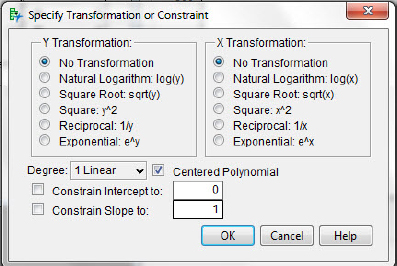
5. Click the Bivariate Fit of 2nd By Actual hot spot and choose Fit Special. The Specify Transformation or Constraint options will appear as in figure 5.10. Choose Square Root sqrt(x).
6. Repeat step 4, except choose Natural Logarithm: log(x).
Figure 5.10 Choosing transformations
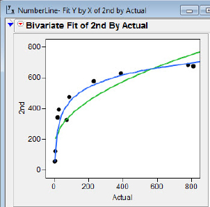
With both fits displayed we can compare the results of the two different transformations as shown in figure 5.11. You can experiment with different colors for the lines by right-clicking on the graph and choosing Customize. The fits will have different colored lines, and in practice you can tell which is which by consulting the colors of the line segments shown at the bottom of the displayed fits. It appears that the logarithmic fit is the better fit to the data, consistent with the reasoning of Opfer and Siegler. JMP calculates the coefficients of determination (r2) for the logarithmic and square root fit for second graders to be 0.95 and 0.80, respectively, suggesting the logarithmic fit is the better one from a raw numerical standpoint.
Figure 5.11 Ln and square root fit
Using the logarithmic model, I will offer an opportunity to practice using the techniques just discussed. In addition to data on second graders, Opfer and Siegler gathered data on the performance of fourth and sixth graders. They hypothesized that as the children grew from second to fourth to sixth grade a logarithmic model would be less appropriate and a straight-line model would better reflect the children’s responses. The data for the three grades are in the file NumberLine.jmp.
1. Select Analyze → Fit Y by X.
2. Select Actual → X, Factor.
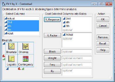
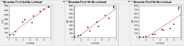
3. Select each of 2nd, 4th, and 6th for Y, Response as shown in figure 5.12.
Figure 5.12 Choosing three grades
Change the horizontal and vertical scales on each of the graphs to be consistent with those shown in figure 5.13 and fit both the straight-line model and the logarithmic model in each graph.
Figure 5.13 The three grades fitted
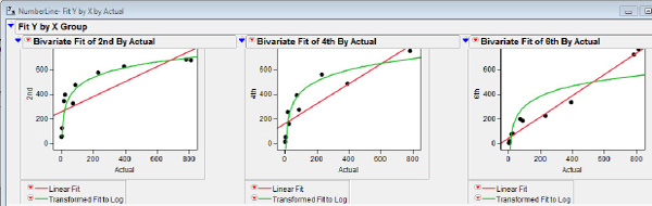
The increasing estimation accuracy as children progress through the grades leads us to believe that older children have a more developed understanding of an interval scale. The changes in coefficients of determination for the two sets of fit, shown in table 5.1, are also consistent with a transition in estimation skills that shifts from one better modeled by a logarithmic model to one better modeled by a straight-line model.
Table 5.1 Coefficients of determination for linear and logarithmic models
| Grade | Linear r2 | Log r2 |
| 2nd | 0.63 | 0.95 |
| 4th | 0.82 | 0.93 |
| 6th | 0.97 | 0.78 |
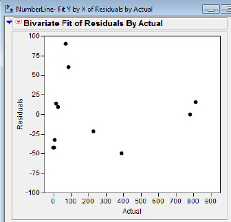
Interestingly, the residual plot of the sixth-grade data shown in figure 5.14 provides additional insight about the increase in understanding that is not readily apparent in the scatterplot of the data. The residuals are more varied, with larger residuals for Actual values near zero; this suggests that estimation skills may not be fully developed even in grade six. The investigators also ran trials with adults, providing an opportunity to check this conjecture.
Figure 5.14 Residual plot, sixth grade
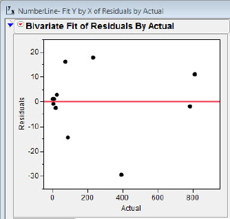
The scatterplot and residual plots, 5.15(a) and 5.15(b), are consistent with the idea that eventually adults develop a “linear representation” of estimation skills. The coefficient of determination for the straight-line fit for adults is a sizzling 0.998, and the residuals appear to have settled down to relatively homogeneous bliss across the spectrum of the Actual values. (If anything, the residuals for Actual values near zero seem to be smallest for Actual values near zero.)
Figure 5.15(a) Regression, adult versus actual
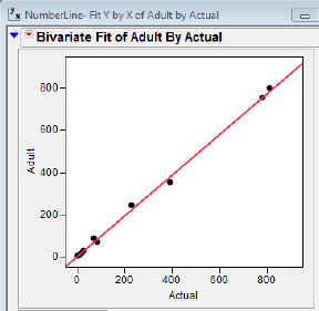
Figure 5.15(b) Residual plot
The Log Model Redux: α + βln(x)
Our discussion of transformations for the α + βln(x) model has been guided mostly by the context of the problem. Opfer and Siegler’s analysis of the development of estimation skills on the number line involved children’s progression through time from a logarithmic representation to a linear representation of the responses to the number line problem. In figure 5.13 we could see this growth “unfolding” from grade two through adulthood.
In elementary statistics classes it is common to take a slightly different technology tack with transformations as students extend their regression skills beyond the straight-line model, y = α + βx. That tack is to algebraically force the nonlinear models into a more familiar “linear” form and treat the models as straight lines. The general idea is that explicit use of transformations helps students understand what is going on “under the hood.” The transforming process begins with the explicit definition of a transformation of a variable and ends with the recognition that the transformation allows us to use already existing techniques via a newly created straight-line model.
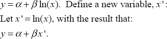
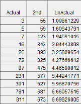
This resulting model is then treated as a straight-line model for purposes of analysis. Using the data from Opfer and Siegler’s grade two, we created a new, transformed variable, LnActual. The results are shown in figure 5.16.
Figure 5.16 Transformed data
Then we fit a straight-line model to the data, as shown in figure 5.17(a). The logarithmic model fitted previously is also presented for comparison in figure 5.17(b).
Figure 5.17(a) Straight-line plot
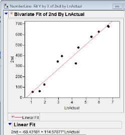
Figure 5.17(b) Ln plot
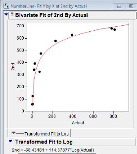
Notice that the equations of the best-fit functions are the same; the x-axis scale and the shape of the graph have been changed, essentially because of the new “scale” introduced by the transformation. Where before the Actual numbers graced the x-axis, we now have natural logs of Actual (see figure 5.18).
Figure 5.18 Linear fits, grades versus LnActual
The Exponential Model: y = αeβx
Another model that is amenable to using logarithmic transformations is the exponential model. Since this model very frequently appears in biological and ecological studies, I will make use of a context taken from those fields: the mating of frogs.
Mating systems in the variety of species in the animal kingdom are incredibly varied (Alcock, 2002). One common mating system is known as lek polygyny. A lek is a cluster of males gathered in a relatively small area to exhibit courtship displays. The display area itself has no apparent particular value to the females, and their subsequent appearance is for the sole purpose of choosing a mate.
Three major hypotheses about the forces that drive this lek behavior have been proposed. One, the “hotspot” hypothesis, is that males position themselves at particular points (hotspots) along routes of females' typical travel. Two, the “hotshot” hypothesis, is that less attractive males gather with more attractive males (hotshots) to have a chance to be seen or perhaps to intercept females heading for more attractive males.
The third hypothesis is the “female preference” hypothesis. The theory here is that females will prefer larger leks over smaller leks, and it is this preference that drives the males to gather. From the female perspective a larger lek is efficient: She can inspect a greater number of males in less time. In addition, she has a smaller risk of predation in a larger gathering. If female preference is operating, one consequence is that the larger leks should attract proportionally more females; that is, in a larger lek the female to male ratio should be greater. We will investigate this third hypothesis.
Murphy (2002) studied lek behavior of barking tree frogs (Hyla gratiosa) and presented three years' worth of data. Data from one of those years, 1987, is presented in the JMP file FrogLeks. (Sorry, couldn’t resist the pun.) The data consist of the numbers of males and the numbers of females observed in two ponds over many nights. I fit a simple linear model, y = α + βx, to the data with result shown in figures 5.19(a) and 5.19(b).
Figure 5.19(a) Fit of female versus male counts
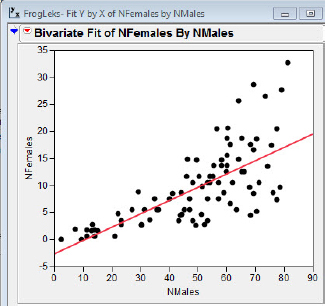
Figure 5.19(b) Residual plot
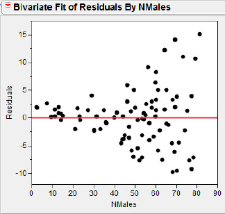
It is clear from the plot that the homogeneity of errors assumption is violated for these data, and the simple linear model will not be appropriate in an inference context. Although we do not necessarily see any obvious curvature in the data, the larger spread of residuals for larger numbers of males in a lek is consistent with an exponential relation, y = αeβx. We can linearize this relation using the following algebraic steps:
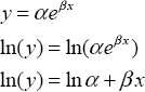
This result suggests the transformation, y' = ln(y). Recall in chapter 3 that we created a new variable by entering a formula that defined a function of existing variables. We will perform this procedure again.
1. Click Cols → New Column to bring up the New Column panel.
We want to create a new variable, the natural log of the number of females, but we notice that there is a slight problem: Some data points have 0 females, a difficulty for log functions! Our workaround in this situation is to create a variable, y' = ln(y +1). This has the effect of translating the graph vertically from y' = ln(y), but the shape of the plot will be unaltered.
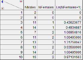
2. In the Column Name field of the New Column panel, type: Ln(NFemales+1).
3. Click Column Properties → Formula → Edit Formula.
4. Click Transcendental → Log → NFemales → + → 1 and close the windows to get back to the JMP data table.
Check to make sure we are agreeing with the formula. The first few lines should appear as in figure 5.20.
Figure 5.20 Check for agreement
Now find the best fit line, ![]() = a + bx and plot the residuals. You should see something like that shown in figure 5.21(a).
= a + bx and plot the residuals. You should see something like that shown in figure 5.21(a).
Figure 5.21(a) NFemales transformed
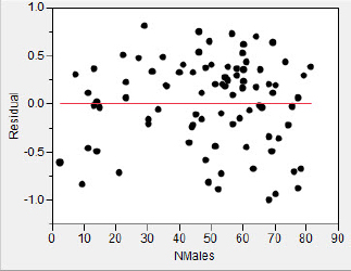
The logarithmic transformation has resulted in residuals that appear to be homogeneous across the number of males in the lek. The slope of the best fit line is positive but not very large, suggesting that the increase in number of females per unit change in the log of the number of males is modest. Perhaps a different perspective on the data may be instructive. We might have reasoned that if the female preference hypothesis is correct, and the number of females in a lek increases at a faster rate than the number of males, then the female-to-male ratio should increase with an increase in the number of males. Let’s follow this alternate path. Close any open windows and return to the JMP data table.
1. In the Column Name field of the New Column panel, type: F/M Ratio.
2. Click Column Properties → Formula → Edit Formula.
3. Click NFemales → ÷ → NMales.
Once again find the best fit line, this time for ![]() = a + b (NMales) and plot the residuals. Your results should agree with those shown in figure 5.21(b).
= a + b (NMales) and plot the residuals. Your results should agree with those shown in figure 5.21(b).
Figure 5.21(b) Ratio transformation
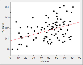
The two analyses are in agreement; the number of females is increasing with the number of males in the lek, consistent with the female preference hypothesis. We should point out that the female preference hypothesis is a causal theory; that is, it is the larger number of males that “causes” the females to prefer joining the lek. However, we have only demonstrated a positive relation with our analysis. In the interest of full disclosure, it should be said that Murphy’s (2002) more advanced multivariate analysis in fact casts some doubt on the female preference hypothesis, at least for these creatures.
Our analyses of these data have demonstrated the ease with which data analysts can transform data using JMP, as well as create new variables on the fly, through an intuitive and simple process. Recall that the idea of creating a variable for the ratio of Females to Males did not actually occur to us until after we had performed our initial transformation and regression, and took a new analytical tactical approach. This illustrates a major strength of JMP: JMP responds to new data analysis ideas as they present themselves, helping the analyst explore the data as the results of the unfolding analysis dictate.
The Power Model: y = αxβ
To illustrate the third common model of data that is amenable to the log transformation, the “power” model, we will return to the data from Jeanne and Nordheim (1996) in the file UnusualWasps. Recall that these investigators studied the behavior of Polybia occidentalis, a social wasp found in Costa Rica. We can also use these data to explore the use of transformations to minimize the influence of outlying points on the regression. We are interested in the number of cells in these creatures' hives. When studying wasp productivity it would be very time consuming to disassemble the hive and count the number of cells, and we hope to find an easier alternative. If the major component of a nest is the collection of cells with only a small amount of dirt or other incidental material brought in, might we be able to simply weigh the nest and use a regression equation to predict the number of cells? Figure 5.22(a) presents a regression of Cells (number of cells) on Total Nest Weight, and Figure 5.22(b) shows its associated residual plot.
Figure 5.22(a) Unusual wasps regression
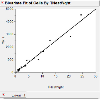
Figure 5.22(b) Unusual wasps plot
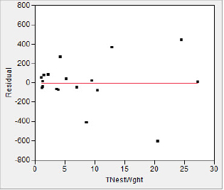
To follow along:
1. Select Fit Y by X to get the regression line.
2. Hide the Analysis of Variance and Parameter Estimates.
3. Click the Linear Fit context arrow to Plot residuals.
In the Summary of Fit we see that the RSquare is 0.97, indicating apparent success in fitting a straight line to data. However, we also notice that those two nests with Total Nest Weights above 20 are a bit unnervingly far away from the mean Total Nest Weight; although they are very close to the best fit line, they may be exerting significantly more influence than the points closer to (0, 0). Furthermore, the residual plot suggests a difference between the size of the residuals for nests with Total Nest Weights below 10 and those nests with a Total Nest Weight of over 10. It is not difficult to isolate the problem; we see in figure 5.23 that the distributions of both number of cells and the total nest weight are skewed.
Figure 5.23 Indications of skew
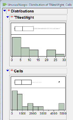
The standard fix for this situation is to implement a logarithmic transformation of both variables and perform the regression analysis on the logarithms of the variables.
We can linearize the power relation as per the following algebra:
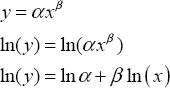
This suggests the transformations, y' = ln(y) and x' = ln(x).
1. Click Column → New Column to bring up the New Column panel.
We would like to create two new variables, the natural log of the number of cells, and the natural log of the total nest weight.
2. In the Column Name field of the New Column panel, type: LnCells.
3. Click Column Properties → Formula → Edit Formula.
4. Select Transcendental → Log → Cells → OK → OK, and close the windows to get back to the JMP data table.
5. In the Column Name field of the New Column panel, type: LogTNestWght. Then click Column Properties → Formula → Edit Formula → Transcendental → Log → NestWght → OK → OK, and close the windows to get back to the JMP data table.
Check Figure 5.24 to make sure we are on the same page.
Figure 5.24 Post-transformed data
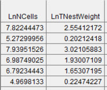
Now find the best fit line, In![]() = a + bln(x) and plot the residuals. You should see something similar to figure 5.25.
= a + bln(x) and plot the residuals. You should see something similar to figure 5.25.
Figure 5.25 Power regression
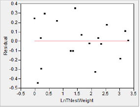
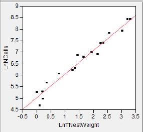
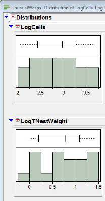
The transformations of both variables using logs has resulted in residuals which appear to be homogeneous across the number of cells. The unequal influence problem has been lessened also, as we can see in figure 5.25; there is less skew in the distribution of both variables.
Figure 5.26 Symmetric data
What Have We Learned?
In chapter 5 I focused on some pesky problems that can arise when we use real data to illustrate the analysis of a simple straight-line model. These problems generally turned out to be of two kinds: (a) a few points straying from the general pattern of points, and (b) whole patterns of points doing so. I discussed the identification and display of influential and outlying points for further analysis and for teaching purposes, as well as the facility within JMP with nonlinear relations. We also analyzed three common transformations to achieve linearity using logarithmic transformations in a bivariate setting.
References
Alcock, J. (2002). Animal behavior: An evolutionary approach (7th ed). Sunderland, MA: Sinauer Associates.
Brodeur, V., et al. (2008). Habitat selection by black bears in an intensively logged boreal forest. Canadian Journal of Zoology 86:1307.
Hawkins, D. (1980). Identification of outliers. London: Chapman & Hall.
Jeanne, R. L., & E. V. Nordheim. (1996). Productivity in a social wasp: Per capita output increases with swarm size. Behavioral Ecology 7(1):43–48.
Kutner, M. H., et al. (2005). Applied linear statistical models (5th ed.). New York: McGraw-Hill.
Montgomery, D. C., E. A. Peck, & G. G. Vining. (2006). Introduction to linear regression analysis (4th ed.). Hoboken, NJ: John Wiley & Sons.
Murphy, C. G. (2002). The cause of correlations between nightly numbers of male and female barking treefrogs (Hyla gratiosa) attending choruses. Behavioral Ecology 14(2):274–81.
NCTM (1980). An agenda for action: Recommendations for school mathematics of the 1980s. Reston, VA: National Council of Teachers of Mathematics.
NCTM (1989). Curriculum and evaluation standards for school mathematics. Reston, VA: National Council of Teachers of Mathematics.
NCTM (2000). Principles and standards for school mathematics: Higher standards for our students, higher standards for ourselves. Washington, DC: National Council of Teachers of Mathematics.
Opfer, J. E. (n.d.). Analyzing the number-line task: A tutorial. Available at: http://www.psy.cmu.edu/~siegler/SiegOpfer03Tut.pdf. Accessed 22 August 2011.
Opfer, J. E., & R. S. Siegler (2007). Representational change and children’s numerical estimation. Cognitive Psychology 55:169–95.
Weisberg, S. (1983). Some principles for regression diagnostics and influence analysis. Technometrics 25(3):240–44.