CHAPTER 7

Reduced-Form versus Structural Models of Credit Risk: A Case Study of Three Models

Navneet Arora,^a Jeffrey R. Bohn,^a,* and Fanlin Zhu^a

1. INTRODUCTION

Complete “realism” is clearly unattainable, and the question whether a theory is realistic “enough” can be settled only by seeing whether it yields predictions that are good enough for the purpose in hand or that are better than predictions from alternative theories (Friedman, 1953).

This insight presented decades ago applies to the current debate regarding structural and reduced-form models. While much of the debate rages about assumptions and theory, relatively little is written about the empirical application of these models. The research results highlighted in this chapter improve our understanding of the empirical performance of several widely known credit pricing models. In this way, we can better evaluate whether particular models are good enough for our collective purpose(s) in hand. Let us begin this discussion by considering some of the key theoretical frameworks developed for modeling credit risk.

Credit pricing models changed forever with the insights of Black and Scholes (1973) and Merton (1974). Jones et al. (1984) punctured the promise of these “structural” models of default by showing how these types of models systematically underestimated observed spreads. Their research reflected a sample of firms with simple capital structures observed during the period 1977–1981. Ogden (1987) confirmed this result, finding that the Merton model underpredicted spreads over US Treasuries by an average of 104 basis points. KMV (now Moody’s–KMV or MKMV) revived the practical applicability of structural models by implementing a modified structural model called the Vasicek–Kealhofer (VK) model (see Vasicek, 1984; Crosbie and Bohn, 2003; Kealhofer, 2003a,b). This VK model is combined with an empirical distribution of distance-to-default to generate the commercially available Expected Default Frequency™ or EDF™ credit measure. The VK model builds on insights gleaned from modifications to the classical structural model suggested by other researchers. Black and Cox (1976) model the default point as an absorbing barrier. Geske (1977) treats the liability claims as compound options. In this framework, Geske assumes the firm has the option to issue new equity to service debt. Longstaff and Schwartz (1995) introduce stochastic interest rates into the structural model framework to create a two-factor specification. Leland and Toft (1996) consider the impact of bankruptcy costs and taxes on the structural model output. In their framework, they assume the firm issues a constant amount of debt continuously with fixed maturity and continuous coupon payments. Collin-Dufresne and Goldstein (2001) extend the Longstaff and Schwartz model by introducing a stationary leverage ratio, allowing firms to deviate from their target leverage ratio in the short run only.

While empirical evidence is still scant, a few empirical researchers have begun to test these model extensions. Lyden and Saraniti (2000) compare the Merton and the Longstaff–Schwartz models and find that both models underpredict spreads; the assumption of stochastic interest rates does not seem to change the qualitative nature of the finding. Eom et al. (2003) find evidence contradicting conventional wisdom on the bias of structural model spreads. They find structural models that depart from the Merton framework tend to overpredict spreads for the debt of firms with high volatility or high leverage. For safer bonds, these models, with the exception of Leland–Toft, underpredict spreads.

On the commercial side, MKMV offers a version of the VK model applied to valuing corporate securities that is built on a specification of the default-risk-free rate, the market risk premium, liquidity premium, and expected recovery in the context of a structural model. The VK model framework is used to produce default probabilities defined as EDF credit measures and is then extended to produce a full characterization of the value of a credit-risky security. This model appears to produce unbiased robust predictions of corporate bond credit spreads (see Bohn, 2000a,b; Agrawal et al., 2004, for more details). Some important modifications to the typical structural framework include estimation of an implicit corporate-risk-free reference curve instead of using the US Treasury curve. Some of the underprediction found in the standard testing of the Merton model likely results from choosing the wrong benchmark curve in the sense that the spread over US Treasuries includes more than compensation for just corporate credit risk. The assumption here is that the appropriate corporate default-risk-free curve is closer to the US swap curve (typical estimates are 10–20 basis points less than the US swap curve). The MKMV implementation of the VK model allows for a time-varying market risk premium, which materially improves the performance of the model. Other important modifications to the framework include the specification of a liquidity premium that may be associated with the firm’s access to capital markets and the assumption of a time-varying expected recovery amount. All of these modifications contribute to producing a more usable structural model.

The structural model is particularly useful for practitioners in the credit portfolio and credit risk management fields. The intuitive economic interpretation of the model facilitates consistent discussion regarding a variety of credit risk exposures. Corporate transaction analysis is also possible with the structural model. If an analyst wants to understand the impact on credit quality of increased borrowing, share repurchases, or the acquisition of another firm, the structural model naturally lends itself to understanding the transaction’s implications. In general, the ability to diagnose the inputs and outputs of the structural model in terms of understandable economic variables (e.g., asset volatility as a proxy for business risk and the market’s assessment of an enterprise’s value) facilitates better communication among loan originators, credit analysts, and credit portfolio managers.

The other major thread of credit-risk modeling research focuses on “reduced-form” models of default. This approach assumes a firm’s default time is inaccessible or unpredictable and driven by a default intensity that is a function of latent state variables. Jarrow and Turnbull (1995), Duffie and Singleton (1999), Hull and White (2000), and Jarrow (2001) present detailed explanations of several well-known reduced-form modeling approaches. Many practitioners in the credit trading arena have tended to gravitate toward this modeling approach, given its mathematical tractability. Jarrow and Protter (2004) argue further that reduced-form models are more appropriate in an information theoretic context, given that we are unlikely to have complete information about the default point and expected recovery. Strictly speaking, most structural models assume complete information.¹ Jarrow and Protter’s claim rests on the premise that a modeler has only as much information as the market, making the reduced-form approach more realistic. In practice, however, the complete information assumption in structural models is an approximation designed to facilitate a simpler way of capturing the various economic nuances of how a firm operates. The strength or weakness of a model should be evaluated on its usefulness in real-world applications. A reduced-form model, while not compromising on the theoretical issue of complete information, suffers from other weaknesses including lack of clear economic rationale for defining the nature of the default process.

An alternative way of characterizing the differences between the two models is that structural models are closer to models that use fundamentals for pricing, whereas reduced-form models are closer to models that rely on relative pricing. Reduced-form models are characterized by flexibility in their functional form. This flexibility is both a strength and a weakness. Given the flexible structure in the functional form for reduced-form models, fitting a narrow collection of credit spreads is straightforward. However, this flexibility in functional form may result in a model with strong in-sample fitting properties, but poor out-of-sample predictive ability. Since this type of model reflects a framework not directly rooted in an explanation of why a firm defaults (i.e., less grounded in the economics driving default than in mathematical tractability), diagnosing how to improve performance of these models can be challenging. In addition, difficulties in interpretation of results can be acute when modeling large cross sections of debt instruments—particularly when there is a high degree of heterogeneity in terms of credit quality. Without empirically testing the costs and benefits of any particular modeling approach, it is premature to draw conclusions based on purely theoretical arguments.

The empirical testing of reduced-form models is still nascent. The reason relates back to the lack of theoretical guidance on characterizing the default intensity process. Duffie (1999) found that the parameter estimates using a square-root process of intensity can be fairly unstable. Another reason relates to the bond data on which these models are usually calibrated. These data are typically indicative, creating data problems like a slow “leakage” of information into the price, thereby producing misleading results.² Transaction bond price sources like the Trade Reporting and Compliance Engine (TRACE) may alleviate data problems, but these sources are new and do not provide detailed time series of data. Other sources of bond data continue to be plagued by missing and inaccurate data. A final reason involves the difficulty in empirically separating the merits of the modeling framework and the quality of the underlying data, given that bond data are typically used to fit the model as well as test the model. Structural models are primarily based on equity price data and will not suffer from this difficulty when they are then tested on bond data. The recent availability of credit default swap data provides a new opportunity to understand the power of both the structural and reduced-form modeling frameworks.³

The crucial question for academicians and practitioners alike is which modeling approach is better in terms of discriminating defaulters from nondefaulters and identifying relative value?

The objective of this chapter is to shed empirical light on this question. We test the performance of a classic Merton model, the VK structural model as implemented by MKMV, and a reduced-form model based on Hull and White (2000) (HW) in separating defaulting and nondefaulting firms in the sample (also known as power-curve testing). We also look at the three models’ performance in explaining the levels and cross-sectional variance of credit default swap data. These three models are chosen because they represent three key stages of the development of the literature in credit risk modeling. The Merton model was the original quantitative structural approach for credit risk modeling. The VK model represents a more realistic and meaningful model for practitioners. (This model was the first commercially marketed structural model.) The HW model is a reduced-form approach that was developed to address parameter stability problems associated with existing approaches as described in Duffie (1999).

The choice of credit default swap data for testing ensures a neutral ground on which the success of the different models can be evaluated. None of the models is calibrated on the data used for testing. This testing strategy enables us to avoid the pitfalls of testing models on data similar to the data used to fit the models. In this way, we conduct a fair out-of-sample test.⁴

The chapter is arranged as follows: Section 2 describes the basic methodologies of the Merton, VK, and HW models. Section 3 discusses the data and the empirical methodology used in the tests. Section 4 presents the results. We also elaborate on some of the robustness checks we conducted on our results in this section. Section 5 concludes.

2. MERTON, VASICEK–KEALHOFER, AND HULL–WHITE MODELS

2.1 Merton Model

Merton (1974) introduced the original model that led to the outpouring of research on structural models. Merton modeled a firm’s asset value as a lognormal process and assumed that the firm would default if the asset value, A, fell below a certain default boundary X. The default was allowed at only one point in time, T. The equity, E, of the firm was modeled as a call option on the underlying assets. The value of the equity was given as

where

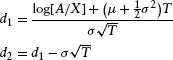
and Φ represents the cumulative normal distribution function. The debt value, D, is then given by

The spread can be computed as

where A is the initial asset value of the firm, X is the default barrier for the firm (i.e., if the firm’s asset value A is below X at the terminal date T, then the firm is in default), μ is the drift of the asset return, and σ is the volatility of the asset returns.

We include this model in our analysis to start with a simple framework as an initial benchmark. A comparison of the performance of a Merton model with the MKMV implementation of the VK model (which reflects substantial modification to the basic Merton framework) will illuminate the impact of relaxing many of the constraining assumptions in the Merton framework.

2.2 VK Model

MKMV provides a term structure of physical default risk probabilities using the VK model. This model treats equity as a perpetual down-and-out option on the underlying assets of a firm. This model accommodates five different types of liabilities: short-term liabilities, long-term liabilities, convertible debt, preferred equity, and common equity. MKMV uses the option-pricing equations derived in the VK framework to obtain the market value of a firm’s assets and its associated asset volatility. The default point term structure (i.e., the default barrier at different points in time in the future) is determined empirically. MKMV combines market asset value, asset volatility, and the default point term structure to calculate a distance-to-default (DD) term structure. This term structure is translated into a physical default probability, better known as an EDF credit measure, using an empirical mapping between DD and historical default data

X_T in the VK model has a slightly different interpretation than in the Merton model. In the context of the VK model framework, if the firm’s market asset value A falls below X_T at any point in time, then the firm is considered to be in default. In the DD-to-EDF empirical mapping step, MKMV uses the VK model to estimate a term structure of this default barrier to generate a DD term structure that can be mapped to a default-probability term structure—hence the subscript T for the default barrier X. The basic methodology is discussed in Crosbie and Bohn (2003), Kealhofer (2003a), and Vasicek (1984). This model departs from the traditional structural model in many ways. First, it treats the firm as a perpetual entity that is continuously borrowing and retiring debt. Second, by explicitly handling different classes of liabilities, it is able to capture richer nuances of the capital structure. Third, it calculates its interim asset volatility by generating asset returns through a de-levering of equity returns. This calculation is different from more common approaches that compute equity volatility and then de-lever it to compute asset volatility. Fourth, MKMV generates the final asset volatility by blending the interim empirical asset volatility as computed in the manner explained above together with a modeled volatility estimated from comparable firms. This step helps filter out noise generated in equity data series. The default probability generated by the MKMV implementation of the VK model is called an expected default frequency or EDF credit measure. These modifications address many of the concerns raised by Eom et al. (2003) regarding the tendency of Merton models to overestimate spreads for riskier bonds and underestimate spreads for safer bonds. This estimation process also results in term structures of default probabilities that are downward-sloping for riskier firms and upward-sloping for safer firms. This pattern is consistent with the empirical credit-migration patterns found in the data.⁵

Once the EDF term structure is obtained, a related cumulative EDF term structure can be calculated up to any term T referred to as CEDF_T. This is then converted to a risk-neutral cumulative default probability CQDF_T using the following equation:

where R² is the square of correlation between the underlying asset returns and the market index returns, and λ is the market Sharpe ratio.⁶

The spread of a zero-coupon bond is obtained as

where LGD stands for the loss given default in a risk-neutral framework. We make two different sets of assumptions for the LGD and market Sharpe ratio in our implementation of the VK model for the purposes of valuation:

• A fixed value of 0.55 for LGD and a value of 0.4 for the market Sharpe ratio. These choices are consistent with the overall historical estimates of the market Sharpe ratio at MKMV (see Agrawal et al., 2004). The level is also generally consistent with estimates from the equity markets. The LGD estimate is consistent with typical recoveries indicated in defaulted bond data.
• A sector- 888and seniority-wise constant LGD, calibrated from the aggregated cross-sectional bonds on any given day. To calibrate, one has to first have a typical value of the LGD for the entire sample. A value of 0.55 for LGD is assumed to do this calibration. Using this assumed value of 0.55, one can calibrate the market Sharpe ratio from bond data. After substituting the value of the Sharpe ratio, one can calibrate the sector- and seniority-specific LGD. This approach is described in detail in Agrawal et al. (2004).

Our findings are robust to both assumptions.⁷ In this chapter, we report only the results based on using the MKMV-supplied EIS (EDF-implied spreads), which assumes the second approach. Note that the floating leg of a simple CDS (i.e., a single payment of LGD paid out at the end of the contract with a probability of CQDF_T) can also be approximated with this relationship.

2.3 HW Model

Hull and White (2000) provide a methodology for valuing credit default swaps when the payoff is contingent on default by a single reference entity and there is no counterparty default risk. Instead of using a hazard rate for the default probability, this model incorporates a default density concept, which is the unconditional cumulative default probability within a period regardless of what happens in other periods. By assuming an expected recovery rate, the model generates default densities recursively based on a set of zero-coupon corporate bond prices and a set of zero-coupon Treasury bond prices. Then the default density term structure is used to calculate the premium of a credit default swap contract. The two sets of zero-coupon bond prices can be bootstrapped from corporate coupon bond prices and Treasury coupon bond prices.

They show the credit default swap (CDS) spread s to be

where T is the life of the CDS contract, q(t) is the risk-neutral default probability density at time t, A(t) is the accrued interest on the reference obligation at time t as a percentage of face value, π is the risk-neutral probability of no credit event over the life of the CDS contract, w is the total payments per year made by the protection buyer, e(t) is the present value of the accrued payment from previous payment date to current date, u(t) is the present value of the payments at time t at the rate of $1 on the payment dates, and is the expected recovery rate on the reference obligation in a risk-neutral world.

The risk-neutral default probability density is obtained from the bond data using the relationship

where α_ij is the present value of the loss on a defaultable bond j relative to an equivalent default-free bond at time t_i. α_ij can be described as

C_j is the claim made on the jth bond in the event of default at time t_i, while R_j is the recovery rate on that claim, F_j is the risk-free value of an equivalent default-free bond at time t_i, while v(t_i) is the present value of a sure payment of $1 at time t_i.

In this framework, one can infer a risk-neutral default risk density from a cross section of bonds with various maturities. As long as the bonds measure the inherent credit risk and have the same recovery as used in the CDS, one should be able to recover a fair price for the CDS based on the prices of the obligor’s traded bonds.

3. DATA AND EMPIRICAL METHODOLOGY

3.1 Data

The data set consists of bond data for each model’s implementation, as described in the preceding section, combined with data on actual CDS spreads used to test each model’s predicted prices. Corporate bond data were provided by EJV, a subsidiary of Reuters. The data include prices quoted daily from 10/02/2000 to 6/30/2004. We selected US dollar-denominated corporate bonds only. There are 706 firms that have at least two bonds that can be used for bootstrapping. CDS data are from CreditTrade and GFInet, two active CDS brokers. Of the 706 firms, 542 firms have CDS data. Therefore, we restricted our analysis to these 542 firms. The final sample tested represented a reasonable cross section of firms with traded debt and equity mitigating concerns about biases arising from sample selection. While the EJV data are indicative in nature and subject to the price “staleness” concerns described above, the CDS data are likely to be closer to actual transacted prices. (CDSs tend to trade more often than bonds.) The lagging nature of the bond data will be somewhat of a handicap for the HW reduced-form model calibrated on those data. Part of the objective of this study is to present model estimations as they would be done in practice so the nature of the available data is as relevant as the estimation approach.

The Merton default probabilities and implied spreads are generated using time series of equity data and financial statements on the sample of firms from COMPUSTAT. The VK daily default probabilities are MKMV EDF credit measures.

The period of study is particularly interesting as it covers two years of recession in many industrialized countries and includes several firms with substantial credit deterioration (e.g., Ahold, Fiat, Ford, Nortel, and Sprint). This time period also includes firms embroiled in major accounting and corporate governance scandals, such as Enron and WorldCom. We required each firm to have a minimum of two bonds to be included in our data set. The highest number of bonds tracked for any particular issuer in this data set is 24.

3.2 Methodology

For the Merton model, we used the default point as 80% of the overall liabilities of the firm. We chose this number because it performed the best in terms of default predictive power. The concept of default predictive power is discussed in the next section. Regardless, we tested other default point specifications and found that the qualitative nature of the results are not sensitive to how we specify the default point.

For the reduced-form model, we first derived the corporate zero rates⁸ by bootstrapping. This procedure facilitates calculating zero-coupon yield curves from market data. For each firm, all senior-unsecured straight bonds (i.e., bonds without embedded options, such as those derived from convertibility and callability) are ranked by their time to maturity from 0 to 6 years. For each 3-month interval, one bond at most is selected. To estimate the zero rate, the firm must have at least two bonds outstanding with suitable price data.

The bootstrapping procedure is done using a MATLAB financial Toolbox function that takes bond prices, coupon rates, maturities, and coupon frequencies as inputs. The procedure is described in detail in Hull (1999). Using this procedure, we obtain zero rates corresponding to relevant bond maturities.

Since many firms have two to five bonds and the zero rates from bootstrapping are very noisy, a linear interpolation of these zero rates may lead to unrealistic forward rates. To mitigate this issue, we use a two-degree polynomial function to approximate the zero curve. We then use the fitted function to generate the zero rates every 3 months. Corporate zero-coupon bond prices are calculated using the 3-month-interval zero rates.

We obtain the Treasury zero rates from 1 month to 30 years from Bloomberg. Treasury zero-coupon bond prices and forward prices are obtained from the risk-free zero curve.

Table 7.1(a) through (c) show the descriptive statistics of the bond and CDS data. In Table 7.1(a), we see that more than 28% of the sample have only two bonds usable for bootstrapping. About 4% of the firms in the sample have more than 20 bonds that were used for bootstrapping. This limited number of bonds per issuer poses difficulties given that the accuracy of the implied default probability density depends on the number of bonds available. Table 7.1(b) shows that the time to maturity of the bonds is fairly uniformly distributed between 0 and 6 years, with the density dropping off at the extremes.

Table 7.1(a) Cumulative Percentage Distribution of Issuers by Number of Bonds Used in Bootstrapping for Zero-Coupon Yield Curve

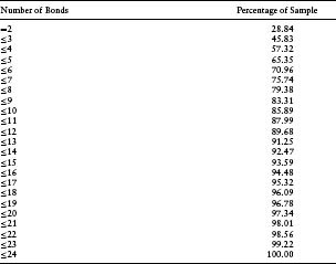
Table 7.1(b) Cumulative Percentage Distribution of Time to Maturity of Bonds Used in Bootstrapping for Zero-Coupon Yield Curve

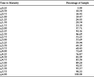
Table 7.1(c) Cumulative Percentage Distribution of CDS by Range of Spreads

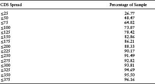
Table 7.1(c) shows that the underlying issuers span a wide cross section of financial health, as measured by CDS spreads.

4. RESULTS

4.1 Default Predictive Power of Models

We first test the ability of the three models to predict defaults. We do this by rank ordering the firms in our sample in their probability of default from highest to lowest. We then eliminate x percent of the riskiest firms from our sample and compute the number of actual defaults that were avoided using this simple rule. This number is expressed as a percentage of the total number of defaults, y%. We vary x from 0 to 100 and find a corresponding y for each x.

Ideally, for a sample of size N with D defaults in it, when x = D/N, then y should be 100%. This would imply that the default predictive model is perfect, that is, each firm eliminated would, in fact, be part of the group that actually defaults. The larger the area under the curve of y against x, the better the model’s power to minimize both Type I error (holding a position in a firm that later defaults) and Type II error (avoiding a position in a firm that does not default). This area is defined as the model’s accuracy ratio (AR) (see Stein, 2002, 2003, for a more detailed discussion of default model performance evaluation). For a random default-risk measure without any predictive power, the x–y graph should be a 45° straight line. The more area between the 45° line and the power curve, the more accurate the measure.

There are two caveats in interpreting results from this test. First, it is a limited sample: Data on bonds and CDSs are restricted to fewer firms than the data available for equities. Of course, a firm that does not issue tradeable bonds may not be as interesting to practitioners; however, the increasing interest in trading bank loans and devising new synthetic credit instruments creates demand for analytics to evaluate instruments for which traded bonds and CDSs are not available. Given the large potential for trading credit risk beyond bonds, the applicability of an equity-based structural model to a much more extensive data set is critical to expanding the coverage of firms and developing market liquidity. The second caveat is that reduced-form models are designed to provide risk-neutral probabilities of default. The order of these may not be the same as that of physical probabilities. For example, a firm with a low physical probability of default but high systematic risk in its asset process may have a higher risk-neutral probability of default compared to a firm with a relatively higher physical probability of default but with no systematic risk in its asset process. As credit investors move toward building portfolios with more optimal return–risk profiles, distinguishing physical from risk-neutral default probabilities becomes critical. In this test, we make the strong assumption that the order stays the same.

FIGURE 7.1(a) shows the results of our default prediction test. In this figure, there are three default-risk measures: default probabilities from a simple Merton structural model, default probabilities from the VK model, and default probabilities from the HW reduced-form model. All three measures are cumulative 1-year risk-neutral default probabilities. As we can see, the VK structural model ranks the highest in its ability to predict default with an AR of 0.801. The HW model approach is not too far behind with an accuracy ratio of 0.785. The basic Merton model, however, is far behind with 0.652. This demonstrates that with proper calibration of default models, both equities and bonds can be effective sources for information about impending defaults.

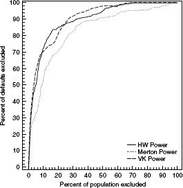
FIGURE 7.1(a) A comparison of predictive power across models as given by the accuracy ratio. The accuracy ratios for the VK model, HW model, and Merton models are 0.801, 0.785, and 0.652, respectively.

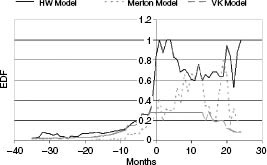
FIGURE 7.1(b) Behavior of risk-neutral default probabilities before default for different models. Date 0 represents the date of default.

FIGURE 7.1(b) shows the median default probabilities from the three models for every defaulted firm in the data set before and after default. Month 0 reflects the month in which each company defaulted. Negative numbers reflect the number of months before default and positive numbers reflect the number of months after default. As we can see from the graph, for the limited sample where the defaulted companies did, in fact, have traded bonds, both the VK model and the reduced-form model predict defaults reasonably well. The classic Merton model trails the other two models in terms of signalling distress closer to the actual event of default.

4.2 Levels and Cross-Sectional Variation in CDS Spreads

We next test the ability of the three models to predict the CDS spread levels and explain the cross-sectional variation in CDS spreads. As discussed above, the conventional wisdom is that structural models, in general, underpredict actual credit spreads. If this were indeed the case, then one would expect that the CDS spreads predicted by the Merton model would generally underestimate the observed level of CDS spreads. For a modified structural approach, such as the VK structural model, previous empirical evidence (see Eom et al., 2003) suggests that one should expect the model implied CDS spreads to be underpredicted for safer firms and overpredicted for riskier firms. Some of this tendency can be explained by the functional form used for transforming physical default probabilities into risk-neutral default probabilities; the function in the VK framework may be increasing the risk-neutral probabilities too much for high-risk firms. That said, the model structure does not imply a particular bias in either direction.

There is no established pattern in the empirical literature with respect to the accuracy or bias of the spreads predicted by reduced-form models. If bond markets are a fair reflection of the inherent risk of a firm and the corporate bond spreads do, in fact, reflect primarily default risk, then the reduced-form model-implied CDS spreads should be an unbiased predictor of CDS spreads. To the extent the reduced-form model is a biased predictor of CDS spreads, the likely cause is factors other than default risk (e.g., liquidity) driving spreads in the corporate bond market.

Figures 7.2(a) through (c) show the performance of the three models in their ability to predict the CDS spreads. The graphs show

Error = Market CDS – Model CDS

as histograms for each model. Consistent with previously published research, we see that the Merton model substantially underpredicts the actual CDS spread, as demonstrated by the right skew of the frequency chart. Both the reduced-form model and the VK structural model seem to be skewed toward the left side, indicating that these models overpredict CDS spreads. However, the skew is much larger for the reduced-form model, with more than 10% of the sample reflecting overestimation of CDS spreads by more than 200 bps. This compares to 3.5% of the sample where the VK structural model overestimates CDS spreads by more than 200 bps.

The median error in the case of the VK structural model is −33.28 bps, which seems to be consistent with the claim of Eom et al. (2003) that more sophisticated structural models overestimate credit risk. This bias is smaller than the median error of −72.71 bps found for reduced-form models. Consistent with the existing literature, the median error in the case of the Merton model is a positive 53.99 bps, implying that the Merton model does underestimate credit risk, even when measured by CDS spreads. Note also that the VK model generated the smallest median absolute error (Table 7.2).

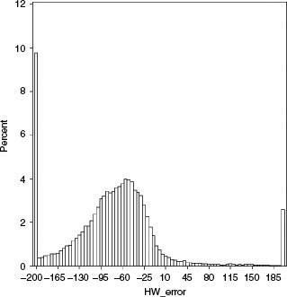
FIGURE 7.2(a) Histogram of difference between the market and the model CDS prices (as given by Market CDS – Model CDS) for HW reduced-form model.

Table 7.2(a) Difference between Market CDS and Model CDS Prices (as given by Market CDS–Model CDS) for Firms in Different CDS Buckets

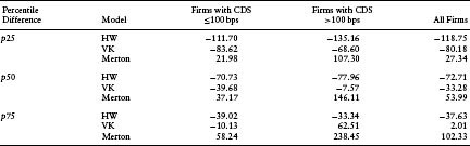
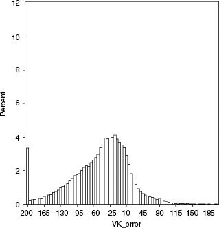
FIGURE 7.2(b) Histogram of difference between the market and the model CDS prices (as given by Market CDS–Model CDS) for the VK structural model.

Table 7.2(b) Difference between Market CDS and Model CDS Prices (as Given by Market CDS – Model CDS) for Firms with Different Numbers of Bonds Available

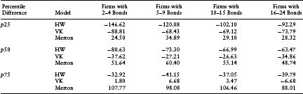
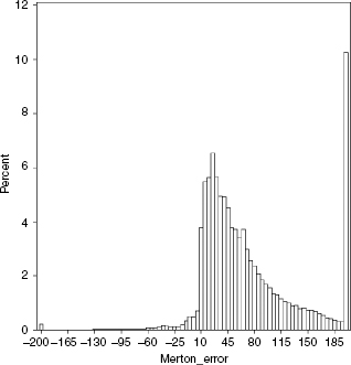
FIGURE 7.2(c) Histogram of difference between the market and the model CDS prices (as given by Market CDS–Model CDS) for Merton model.

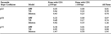
Finally, FIGURE 7.3 shows the time series of the correlation of market CDS spreads with modeled CDS spreads. This correlation reflects the ability of a model to explain the cross-sectional variation of market CDS spreads. If the modeled CDS spreads are the same as the market CDS spreads, then the correlation will be exactly 1. In general, a better correspondence between the levels of modeled and realized market spreads will lead to a higher correlation. As evident from this figure, the VK model performs the best in this regard. Surprisingly, the HW reduced-form model performs the worst. Table 7.3(a) shows the median of the slope coefficients that result from regressing the market CDS on the modeled CDS cross-sectionally on a daily basis. In general, if the model is an unbiased estimator of the realized spread, then this slope should be 1. While both the VK and Merton models deviate from 1, with median slopes of 0.76 and 1.26, respectively, the HW model’s median slope is at 0.07, which seems unusually low. The median R-squareds of these regressions (which should also be the squares of the correlation between the market and modeled spreads) of the HW model, the VK model, and the Merton model stand at 0.09, 0.48, and 0.26, respectively, once again demonstrating the strength of the VK structural model in explaining the cross-sectional variation of CDS spreads.⁹

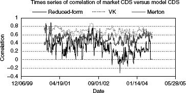
FIGURE 7.3 Time series of correlation between market CDS spreads and model CDS spreads. For each day, the correlation was computed based on cross-sectional data of market and model CDS prices.

Table 7.3(a) Slope Coefficients Resulting from Regression of Market CDSs on Model CDSs by Firms in Different CDS Spread Buckets. The slope coefficients were computed daily for a 3-year period. The different quartiles of the time series distribution of the slope coefficients are reported here

These results are particularly striking, given that VK-model-based EDF credit measures rely mostly on input from equity markets.

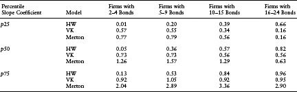
Table 7.3(b) Slope Coefficients Resulting from Regression of Market CDSs on Model CDSs by Firms with Numbers of Bonds Available. The slope coefficients were computed daily for a 3-year period. The different quartiles of the time series distribution of the slope coefficients are reported here

4.3 Further Diagnosis of Results

In an attempt to understand the overall results, we drilled deeper into the nature of the relationship between CDS and bond data. Some market participants and academicians¹⁰ claim that while CDS and equity markets are relatively liquid, the bond markets are more impacted by liquidity problems. If liquidity across these markets differs in this way, one would expect that time to maturity would impact the correlation between bond and CDS prices. Two explanations are possible for this impact. First, bonds that are closer to maturity usually have a low probability of defaulting, and hence a low spread as implied by structural models. Therefore, any spread due to noncredit risk represents a larger fraction of overall bond spread. Since this “noncredit risk component” does not have to necessarily correlate across different markets, bonds with less time to maturity are likely to have lower correlation with their corresponding CDS spreads. Second, bonds with less time to maturity are more likely to be “off-the-run” securities (i.e., the time to maturity of these types of bonds makes them less attractive to market participants focused on matching particular durations) compared to bonds with greater time to maturity. Assuming that “on-the-run” securities are more liquid, bonds with more time to maturity are less likely to be impacted by liquidity problems.

In FIGURE 7.4, we further examine the correlation between the bond and CDS markets by dividing the bonds into three different-tenor buckets:

• 0–2 years
• 2–4 years
• 4–6 years

These correlations are cross-sectional. We also plot the time series behavior of these correlations. Since the daily correlations are too noisy, the plot shows the 5-day moving average. As expected, the correlation is fairly low for the low-maturity bonds. Note that even after calculating a 5-day moving average, the correlations are extremely noisy. Equations 7.8 and 7.9 demonstrate that the zero rates can be highly sensitive to any noise in the data. If one zero rate is adversely affected by noise, the entire term structure of zero rates can be impacted. Low correlations may be a consequence of the noise in the data and not necessarily reflective of each model’s performance.

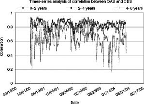
FIGURE 7.4 Time series of correlation between market CDS spreads and bond spreads across different-tenor buckets. For each day, the correlation was computed based on cross-sectional data of market CDS and bond spreads.

An alternative way of testing the reduced-form framework would be to use less noisy data for calibration, that is, CDS data. Unfortunately, at present, most of the CDS contracts are liquid only at the 5-year tenor. Using these data, we would observe a zero rate at only one point on the term structure. Any testing that follows would have to assume a flat term structure for zero rates. Nonetheless, this test would be useful given that the zero-rate term structure would be less sensitive to noise in the data. Therefore, one could alternatively calibrate the data on CDS data and test it on bond data. This test, while interesting, would limit the ability of reduced-form models to capture nonflat term structures of credit risk. Second, this test would only validate the usefulness of pricing bonds with CDS data and not vice versa. The model created by Hull and White (2000) is intended for pricing CDS contracts using bond spreads, not necessarily the other way around. In addition, we acknowledge that it may be possible to achieve superior pricing of CDS contracts using bond data filtered by tenor and other liquidity indicators. Unfortunately, few guidelines exist for creating these filters. We leave construction of these filters and further investigation of these issues to future research.¹¹

4.4 Robustness Tests

In this section, we subject our results to more scrutiny by analyzing various subsets of the data to determine whether our results are attributable to the presence of outliers.

One possible explanation for our results may be that healthier firms behave differently than riskier firms. We again conduct our tests on these two subsets of firms separately. Our proxy for a relatively healthy firm is one where the CDS spread is less than 100 bps. As seen in Table 7.1(c), about 73% of the sample falls in the healthier category. This percentage is in line with our expectations; most of the CDS data are concentrated among larger and less risky firms. Table 7.2(a) shows that the negative bias of the VK model is typically evident for firms with CDS spreads below 100 bps. For riskier firms, the modeled spreads are largely unbiased, with the median error around −7.6 bps. This result is inconsistent with the claim of Eom et al. (2003) that more sophisticated structural models underpredict credit risk at lower levels of risk, and overpredict credit risk at higher levels of credit risk. In comparison, the Merton model consistently underpredicts credit risk, as can be seen by the positive errors for both classes of CDS. The HW reduced-form model overpredicts credit risk for both classes. This overprediction is significantly high and even the 75th percentiles of errors are fairly negative for both classes of CDS.

Table 7.4(a) highlights the ability of the models to explain the cross-sectional variation of CDS spreads. We find that although on aggregate, the HW model is outperformed by the Merton and VK models, on the subset of data with CDS < 100 bps, the HW model outperforms the Merton model. The VK model outperforms the other two models in all other subsets of the data except the 75th percentile of firms with CDS < 100 bps.

One possible explanation for the HW model’s difficulties may involve the fact that most issuers have few outstanding bonds. A larger number of bond issues will increase the efficiency of estimating the default density. To test for this possibility, we divided our sample into firms with two bonds, firms with three to four bonds, firms with five to nine bonds, firms with 10 to 15 bonds, and firms with 16 to 24 bonds.¹²

Table 7.2(b) shows that the negative bias of the VK and HW models is present in all subsamples of the data. This result indicates that the bias is not being caused by firms with few outstanding bonds. The negative bias of the HW model is larger compared to that of the VK model for all data subsets. The Merton model, on the other hand, has a consistently positive bias in all categories, indicating that the model’s underestimation of credit risk is fairly consistent across various subsamples of the data.

Table 7.4(a) Ability of a Model to Explain Cross-Sectional Variation of Market CDS Spreads, Given by R-Squared of Regression of Market CDS on Model CDS by Firms in Different CDS Buckets. The R-squareds were computed daily for a 3-year period. The different quartiles of the time series distribution of R-squareds are reported here

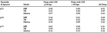
Table 7.4(b) Ability of Model to Explain Cross-Sectional Variation of Market CDS Spreads, Given by R-Squared of Regression of Market CDS on Model CDS by Firms with Different Numbers of Bonds Available. The R-squared was computed daily for a 3-year period. The different quartiles of the time series distribution of R-squareds are reported here

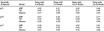
Table 7.4(b) examines the impact of the availability of information, as measured by the number of bonds by an issuer, on the ability of the HW model to explain the cross-sectional variation of the CDS spreads. Interestingly, we find that the HW model outperforms the other two models when there are more than 10 bonds available to calibrate the default probability density. This improvement most likely results from the greater amount of cross-sectional information, in terms of the number of bonds, available to calibrate the default probability density. Similarly, in Table 7.3(b), we see that the sensitivity of the realized CDS spread to the modeled spread, as measured by the median slope of cross-sectional regression of market spreads on model spreads, increases with the number of bonds available.

The ability of both the VK model and the Merton model to explain the cross-sectional variation declines among firms with more than 15 bonds issued, as observed by the lower R-squareds. This result is surprising, given that these models do not use bond information in their calibration. The result is most likely driven by the fact that firms that issue such large numbers of bonds have other variables impacting their spreads (e.g., interest-rate risk). These firms account for only 5% of the data, as seen in Table 7.1(a). That said, in terms of debt outstanding, these firms constitute a larger percentage (but not a majority) of the dollar amount of corporate debt outstanding. For example, on June 2004, firms that had more than 10 bonds used in bootstrapping (after applying all the filters) represented 40% of the total amount outstanding in our sample. Similarly, firms that had more than 15 bonds available for bootstrapping represented about 28% of the amount outstanding. Regardless of the measure, the majority of the firms tested in this research exercise did not have a large number of bonds outstanding.

We have seen that, all else equal, the performance of the model improves with the number of bonds available for bootstrapping. Further characterization of the sample of prolific issuers helps us interpret the results on other drivers of model performance. Large firms tend to be the ones that issue more bonds.¹³ Table 7.5(a) shows that large firms account for relatively more of the prolific issuers than small firms. Large issuers also tend to be less risky. Table 7.5(c) demonstrates this fact by showing the distribution of CDS spreads for the entire sample compared to the distribution of CDS spreads for the largest firms (defined by log(size) > 11). The large-firm sample does, in fact, have a higher percentage of firms with lower CDS spreads. We also find that large issuers tend to issue debt of duration similar to smaller firms. This can be seen from the comparison of the distribution of time to maturity across bonds of large firms and bonds of the overall sample in Table 7.5(b). Therefore, as a percentage contribution to the overall spread, interest rate risk may dwarf default risk for these types of larger and safer issuers. Corporate bonds issued by small firms tend not to be transacted as much, making liquidity risk relatively more important in determining their spreads. These circumstances create countervailing influences on the performance of the HW model using bond data to fit CDS spreads. To the extent that interest rate risk or liquidity risk overpowers default risk as the primary driver of CDS spreads, an HW model calibrated on bond data will not perform as well. Given these circumstances, we cannot predict ex ante how firm size will impact model performance.

We test the impact of size on model performance by further dividing the subsamples based on the number of bonds available for bootstrapping. This procedure is designed to isolate the effect of size from the effect of number of bonds available for bootstrapping (since the two are somewhat positively correlated). For each subsample, we compute the median size of the firms. We then divide each subsample into two groups: one group where firm size exceeds the subsample median and the other group where firm size is less than the subsample median. Table 7.6(a) reports the performance of each model in explaining the cross-sectional variation in CDS spreads (as measured by the R-squareds of the regression of CDS spreads on modeled spreads) across the two size categories for each subsample.

Table 7.5(a) Cumulative Percentage Distribution of Issuers by Number of Bonds Used in Bootstrapping for Zero-Coupon Yield Curve

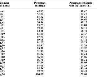
Table 7.5(b) Cumulative Percentage Distribution of Time to Maturity of Bonds Used in Bootstrapping for Zero-Coupon Yield Curve

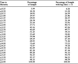
Table 7.5(c) Cumulative Percentage Distribution of CDSs by Range of Spreads

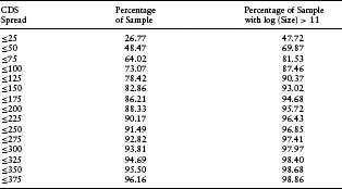
Table 7.6(a) Comparison of Different Models’ Ability to Explain Cross-Sectional Variation (Measured by R-squared of Cross-Sectional Regression of Market CDS on Model CDS Prices) across Large and Small Firms, Controlling for Number of Bonds Available for Bootstrapping. The R-squareds were computed daily for a 3-year period. The different quartiles of the time series distribution of R-squareds are reported here. The asterisk indicates that the cross-sectional correlation between market and model CDS prices is actually negative; there are a large number because R-squared is the square of the correlation here

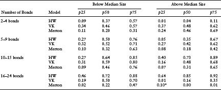
The VK model performs fairly consistently across the different subsamples. The HW model performance is a little more varied. As the number of bonds outstanding increases, the HW model performs progressively better. The classic Merton model consistently underperforms the other models in almost every subsample. One interesting pattern is the HW outperformance for large profilic issuers. We suspect these results reflect the extent to which default risk is not a primary determinant of spreads for large, low-risk, prolific issuers of long-term debt. The performance of the structural models relies on the sensitivity of CDS spreads to changes in the equity-based default probability measures. The standard Merton model reflects primarily equity price movement, which may not be a primary determinant of CDS spreads for large firms. The VK model, on the other hand, includes modifications to the specification of the default point, the estimation of asset volatility, and the interaction of firm asset value and the default model in such a way as to capture more of the determinants of CDS spreads for all firms, regardless of size. As a result, its performance is consistent across subsamples. For the most prolific issuers (i.e., outstanding bonds greater than 16), we should interpret the results with care given the small number in this subsample.

Table 7.6(b) Summary Statistics of CDS Spreads across Firms with Different Numbers of Bond Issues. All statistics were based on daily observations in the period 2000/10 to 2004/06, and the numbers reported here are the medians across the daily time series of summary statistics

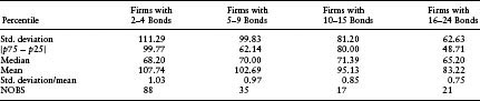
Table 7.6(b) reports some of the characteristics of the cross-sectional distribution of the CDS spreads in this sample, categorized by firms with different numbers of bond issues available. As we move to firms with a larger number of bonds, the CDS spreads are less diverse, as indicated by the standard deviation and the interquartile range (|p75 – p25|) of the spreads. There is also a substantial reduction in the number of CDS observations available on a daily basis (as seen by the median number of observations each day). R-squared is not a reliable statistic when the variation in the dependent variable (in this case, the CDS spreads) is low, or the number of observations is low. Our prolific-issuer subsamples suffer from both of these inadequacies. For example, upon breaking the sample of firms with more than 15 bonds into two halves according to size (as in Table 7.6a), the median daily number of observations in each half is about nine. This, along with the lowest coefficient of variation (standard deviation/mean) leads to an unreliable R-squared measure. The subsamples for firms with fewer numbers of bonds outstanding do not suffer from this particular difficulty. All results should be considered with these characteristics in mind.

In summary, the testing demonstrates that for the vast majority of firms, a structural model such as the VK model developed at MKMV, calibrated on a time series of equity data, works better in measuring credit risk relative to an HW reduced-form model calibrated on a cross section of corporate bonds. The VK model substantially outperforms a simple implementation of the standard Merton model. For practitioners looking across the broad cross section of traded credit instruments, the data requirements for robust reduced-form modeling and the availability of robust equity-based measures should inform discussions of which modeling approach to use. Moreover, users of reduced-form models looking to price other credit-risky securities such as CDSs should bear in mind the potential impact on bond spreads of other risks resulting from interest rate movements and changes in liquidity. These effects can differ across size and spread levels, thereby distorting the performance of these models. A model such as VK is relatively more stable in its performance across various categories by size and spreads. The model’s strength is partially due to its structural framework that uses equity data, which are less contaminated by other risks, and partially due to its more sophisticated implementation.

5. CONCLUSION

In this chapter, we empirically test the success of three models in their ability to measure credit risk. These models are the Merton model, the Vasicek–Kealhofer model, and the Hull–White model. These three models were chosen because they represent three key stages in the development of the theoretical literature in credit risk. These models also represent two main approaches for credit-risk modeling: the structural approach and the reduced-form approach.

This research is the first attempt at comparing these types of models in their ability to discriminate defaulted firms from nondefaulted firms, and to predict the levels and explain the cross-sectional variation of CDS spreads. The advantage of these data is that they are not used in the calibration of any of the models, thereby facilitating a true out-of-sample test.

The VK model marginally outperformed the HW model in terms of its default predictive power. Both of these models consistently outperformed the Merton model in their default predictive power. Despite the advantages stated by proponents of reduced-form models, the HW model largely under-performs a sophisticated structural model (as implemented by MKMV) in its ability to predict levels and explain cross-sectional variation of CDS spreads. Interestingly enough, the HW model outperforms the simple Merton model when a given firm issues a large number of bonds. In these cases of firms issuing more than 10 bonds at any given time, the HW model can also outperform (in terms of explaining the cross-sectional variation of CDS spreads) the more sophisticated VK structural model for some subsets of low-risk corporate issuers. At this time, the number of such firms is small. In our sample, the HW model was more effective in its ability to explain the cross-sectional variation of the CDS spreads only for the largest 5% of the firms, in terms of the number of issues outstanding on which data were available. Even for this sample, the error in terms of the difference between actual and predicted levels of spreads was much larger for the HW model when compared to the VK model. The performance of the VK model is consistent across large and small firms. Surprisingly, the performance of the HW model worsens as it is applied to larger firms that issue few bonds. The performance of the HW model could have been impacted due to the sensitivity of the model calibration to the underlying bond data at various tenors coupled with the propensity of bond data to be “noisier” at shorter terms. In order to improve a reduced-form model’s performance using bond data, better filters will need to be devised to eliminate noisy data, thus facilitating more efficient calibration. We leave this type of investigation to future research. The overall results emphasize the importance of empirical evaluation when assessing the strengths and weaknesses of different types of credit risk models.

ACKNOWLEDGMENTS

The authors would like to thank Deepak Agrawal, Ittiphan Jearkjirm, Stephen Kealhofer, Hans Mikkelsen, Martha Sellers, Roger Stein, Shisheng Qu, Bin Zeng, and seminar participants at MKMV and the Prague Fixed Income Workshop (2004) for invaluable suggestions and advice. We also thank an anonymous referee whose suggestions helped improve the chapter substantially. We are grateful to Jong Park for providing the code involving the implementation of the Merton model. All errors are ours.

NOTES

1. Giesecke and Goldberg (2004) show that it is possible to develop a structural model in which the modeler also has incomplete information about the default point, making the time to default inaccessible even in a structural model. Duffie and Lando (2001) propose a “hybrid” model that assumes accounting information is noisy, thereby making the default time inaccessible in the context of a structural model.

2. Because indicative prices do not always reflect all the information in the market, a researcher may mistakenly conclude that a particular model predicts price changes when, in fact, an actual trade would have reflected an immediate price change, eliminating any predictive power of the model. See Duffie (1999) for more discussion on this problem of stale bond prices.

3. See, for example, Ericsson and Reneby (2004).

4. The three models take different sources of data as inputs. While the Merton and VK models mostly rely on equity data, the HW model is calibrated with bond data. Therefore, any result in this test is a reflection of the framework as well as the quality of data available to the models as input. One of the strengths of a model, especially from a practitioner’s point of view, is that it should yield accurate results based on data that are easily available and accessible. A conceptually powerful framework, while intellectually stimulating, can be fairly meaningless if any application of it relies on data that are either unavailable or of poor quality.

5. Note that Helwege and Turner (1999) find evidence of upward-sloping term structures of spreads for risky corporate bonds. When we look at the behavior of distance-to-default (DD) for firms, the downward-sloping term structures of default probabilities for high-risk issuers appear to be more typical. In other research completed by Agrawal and Bohn (2005), these contradictory findings are reconciled by investigating the differences in par spreads and zero-coupon spreads as well as the differences in spreads calculated from new bond issues and bond issues traded in the secondary market. While Helwege and Turner see upward-sloping term structures in par spreads for new bond issues, the more recent research finds that zero-coupon spreads from the secondary market for high-yield bonds reflect the downward-sloping term structures predicted in the theory and reflected in the DD data. Agrawal and Bohn (2005) also show that under certain conditions zero-coupon spreads can be downward sloping when par spreads are not.

6. The normal and abnormal inverse functions act as translators of the default probability estimate without requiring that the default probability estimate, itself, be generated from a normal distribution. In this case, the CEDF_T represents the physical cumulative default probability and was calculated from the empirical distribution estimated at MKMV. A detailed derivation of this expression can be found in Agrawal et al. (2004).

7. This step helps improve performance of modeled bond spreads against market bond spreads.

8. A zero rate is the implicit interest on a zero-coupon bond of a given maturity.

9. Median R–squareds of 0.09, 0.48, and 0.26 correspond to median correlations of approximately 30%, 70%, and 51%.

10. See Longstaff et al. (2004), for example.

11. We thank an anonymous referee for suggesting most of the ideas in this subsection.

12. The number of bonds represents the number available for bootstrapping after using all the filters described above—not the actual number of bonds outstanding.

13. We measure the size of a firm by its book asset value. A large firm is considered to have book assets in excess of about $60 billion [log (60,000) is approximately 11; our data are reported in millions of dollars].

REFERENCES

Agrawal, D., Arora, N. and Bohn, J. (2004). “Parsimony in Practice: An EDF-Based Model of Credit Spreads.” White Paper, Moody’s KMV.

Agrawal, D. and Bohn, J. (2005). “Humpbacks in Credit Spreads.” White Paper, Moody’s KMV.

Black, F. and Cox, J. (1976). “Valuing Corporate Securities: Some Effects of Bond Indenture Provisions.” Journal of Finance 31, 351–367.

Black, F. and Scholes, M. (1973). “The Pricing of Options and Corporate Liabilities.” Journal of Political Economy 81, 637–659.

Bohn, J. (2000a). “A Survey of Contingent-Claims Approaches to Risky Debt Valuation.” Journal of Risk Finance 1(3), 53–78.

Bohn, J. (2000b). “An Empirical Assessment of a Simple Contingent-Claims Model for the Valuation of Risky Debt.” Journal of Risk Finance 1(4), 55–77.

Collin-Dufresne, P. and Goldstein, R. (2001). “Do Credit Spreads Reflect Stationary Leverage Ratios?” Journal of Finance 56, 1929–1957.

Collin-Dufresne, P., Goldstein, R. and Martin, S. (2001). “The Determinants of Credit Spread Changes.” Journal of Finance 56, 2177–2208.

Crosbie, P. and Bohn, J. (2003). “Modeling Default Risk.” White Paper, Moody’s KMV.

Duffie, G. (1999). “Estimating the Price of Default Risk.” Review of Financial Studies 12(1), 1997–2026.

Duffie, D. and Lando, D. (2001). “Term Structures of Credit Spreads with Incomplete Accounting Information.” Econometrica 69, 633–664.

Duffie, D. and Singleton, K. (1999). “Modeling the Term Structure of Defaultable Bonds.” Review of Financial Studies 12, 687–720.

Eom, Y., Helwege, J. and Huang, J. (2003). “Structural Models of Corporate Bond Pricing: An Empirical Analysis.” Review of Financial Studies.

Ericsson, J. and Reneby, J. (2004). “An Empirical Study of Structural Credit Risk Models Using Stock and Bond Prices.” Institutional Investors Inc., pp. 38–49.

Friedman, M. (1953). The Methodology of Positive Economics. Essay in Essays on Positive Economics, University of Chicago Press.

Geske, R. (1977). “The Valuation of Corporate Liabilities as Compound Options.” Journal of Financial and Quantitative Analysis pp. 541–552.

Giesecke, K. and Goldberg, L. (2004). “Forecasting Default in the Face of Uncertainty.” Journal of Derivatives 12(1), 11–25.

Helwege, J. and Turner, C. (1999). “The Slope of the Credit Yield Curve for Speculative Grade Issuers.” Journal of Finance 54(5), 1869–1884.

Hull, J. and White, A. (2000). “Valuing Credit Default Swaps: No Counterparty Default Risk.” Working Paper, University of Toronto.

Hull, J. (1999). Options, Futures and Other Derivatives, 4th edn. Englewood Cliffs, NJ: Prentice Hall Publications.

Jarrow, R. (2001). “Default Parameter Estimation Using Market Prices.” Financial Analysts Journal 57, 75–92.

Jarrow, R. and Protter, P. (2004). “Structural versus Reduced Form Models: A New Information-Based Perspective.” Working Paper, Cornell University.

Jarrow, R. and Turnbull, S. (1995). “Pricing Derivatives on Financial Securities Subject to Default Risk.” Journal of Finance 50, 53–86.

Kealhofer, S. (2003a). “Quantifying Credit Risk I: Default Prediction.” Financial Analysts Journal, 59(1), 30–44.

Kealhofer, S. (2003b). “Quantifying Credit Risk II: Debt Valuation.” Financial Analysts Journal, 59(3), 78–92.

Kim, J., Ramaswamy, K. and Sunderasan, S. (1993). “Does Default Risk in Coupons Affect the Valuation of Corporate Bonds? A Contingent Claims Model.” Financial Management 22, 117–131.

Leland, H. and Toft, K. (1996). “Optimal Capital Structure, Endogeneous Bankruptcy, and the Term Structure of Credit Spreads.” Journal of Finance 51, 987–1019.

Longstaff, F. and Schwartz, E. (1995). “Valuing Risky Debt: A New Approach.” Journal of Finance 50, 789–820.

Longstaff, F., Mithal, S. and Neis, E. (2004). “Corporate Yield Spreads: Default Risk or Liquidity? New Evidence from the Credit-Default Swap Market.” Working Paper, Anderson School of Management, UCLA.

Lyden, S. and Saraniti, D. (2000). “An Empirical Examination of the Classical Theory of Corporate Security Valuation.” Research Paper, Barclays Global Investors.

Merton, R. (1974). “On the Pricing of Corporate Debt: The Risk Structure of Interest Rates.” Journal of Finance 29, 449–470.

Ogden, J. (1987). “Determinants of the Ratings and Yields on Corporate Bonds: Tests of the Contingent Claim Model.” The Journal of Financial Research 10, 329–339.

Stein, R. (2002). “Benchmarking Default Prediction Models: Pitfalls and Remedies in Model Validation.” White Paper, Moody’s KMV.

Stein, R. (2003). “Are the Probabilities Right? A First Approximation to the Lower Bound on the Number of Observations Required to Test for Default Rate Accuracy.” White Paper, Moody’s KMV.

Vasicek, O. (1984). “Credit Valuation.” White Paper, Moody’s KMV.

Keywords: Credit risk; default risk; default probability; structural mode; reduced-form model; Merton model; equity; corporate bonds; credit default swaps (CDS); power curves; credit spreads

---

^a Research Group, Moody’s KMV, 1620 Montgomery Street, San Francisco, CA 94111, USA.

^*Corresponding author. E-mail: [email protected].