CHAPTER 8

Implications of Correlated Default for Portfolio Allocation to Corporate Bonds

Mark B. Wise^a,* and Vineer Bhansali^b

1. INTRODUCTION

Investors routinely look to the corporate bond market in particular, and to spread markets in general, to enhance the performance of their portfolios. However, for every source of excess return over the risk-free rate, there is a source of excess risk. When sources of risk are correlated, the allocation decision to the risky sectors, as well as allocation to particular securities in that sector, can be substantially different from the uncorrelated case. Since the joint probability distribution of returns of a set of defaultable bonds varies with the joint probabilities of default, recovery fraction for each bond, and number of defaultable bonds, a direct approach to the allocation problem that incorporates all these factors completely can only be attempted numerically within the context of a default model. This approach can have the shortcoming of hiding the intuition behind the asset allocation process in practice, which leans very heavily on the quantification of the first few moments, such as the mean, variance, and skewness. In this chapter, we take the practical approach of characterizing the portfolio default loss distribution in terms of its moment expansion. Focusing on allocation to corporate bonds (the analysis in this chapter can be generalized to any risky sector which has securities with discrete payoffs) we will answer the following questions:

• In the presence of correlated defaults, how well does retaining the first few moments of the portfolio default loss distribution do, for the portfolio allocation problem, as compared to the more intensive full numerical solution?
• For different choices of correlations, probabilities of default, number of bonds in the portfolio, and investment time horizon, how does the optimal allocation to the risky bonds vary?

In this chapter we consider portfolios consisting of risk-free assets at a return y and corporate zero-coupon bonds with return c_i for firm i, and study how correlations between defaults affect the optimal allocation to corporate assets in the portfolio over some time horizon T. We assume that if company i defaults at time t, a fraction R_i (the recovery fraction) of the value of its bonds is recovered and reinvested at the risk-free rate. We quantify the impact of risk associated with losses from corporate defaults¹ on portfolio allocation. To compensate the investor for default risk, the corporate bond's return c_i is greater than that of the risk-free assets in the portfolio. The excess return, or spread of investment in bonds, of firm i can be decomposed into two parts. The first part of the spread, which we call λ_i, arises as the actuarially fair value of assuming the risk of default. The second part, which we call μ_i, is the excess risk premium that compensates the corporate bond investor above and beyond the probabilistically fair value. In practice, μ_i can arise due to a number of features not directly related to defaults. For example, traders will partition μ_i into two pieces, one for liquidity and one for event risk, μ_i = l_i+e_i. Most low-grade bonds may have a full percentage point arising simply from liquidity premiums, and μ_i can fluctuate to large values in periods of credit stress. Liquidity l_i is systematic and one would expect it to be roughly equal for a similar class of bonds. Event risk e_i contributes to μ_i due to the firm's specific vulnerability to factors that affect it (e.g., negative press). In periods of stress, the default probabilities l_i and e_i all increase simultaneously, and the recovery rate expectations R_i fall, leading to a spike in the overall spread. Since these variables can be highly volatile, the reason behind the portfolio approach to managing credit is to minimize the impact of nonsystematic event risk in the portfolio.² The excess risk premium itself is not very stable over time. Empirical research shows that the excess risk premium may vary from tens of basis points to hundreds of basis points. For instance, in the BB asset class, if we assume a recovery rate of 50% and default probability of 2%, the actuarially fair value of the spread is 100 basis points (bp). However, it is not uncommon to find actual spreads of the BB class to be 300 bp over Treasuries (Altman, 1989). The excess 200 bp of risk premium can be decomposed in any combination of liquidity premium and event risk premium, and is best left to the judgment of the market. When the liquidity premium component is small compared to event risk premium, we would expect the portfolio diversification and methods of this chapter to be valuable.

One other factor must be kept in mind when comparing historical spreads to current levels. In the late 80s and early 90s, the spread was routinely quoted in terms of a Treasury benchmark curve. However, the market itself has developed to a point where spreads are quoted over both the LIBOR swap rate and the Treasury rate, and the swap rate has gradually substituted the Treasury rate as the risk-free benchmark curve. This has two impacts. First, since the swap spread (swap rate minus Treasury rate for a given maturity) in the US is significant (of the order of 50 bp as of this writing), the excess spread must be computed as a difference to the swap yield curve. Second, the swap spread itself has been very volatile during the last few years, which leads to an added source of non-default-related risk in the spread of corporate bonds when computed against the Treasury curve. Thus, the 200 bp of residual spread is effectively 150 bp over the swap rate in the BB example, of which, for lack of better knowledge, equal amounts may be assumed to arise from liquidity and event risk premium over the long term. The allocation decision to risky bonds strongly depends on the level of risk aversion in the investor's utility function, and the required spread for a given allocation will go up nonlinearly as risk aversion increases.

The value of the optimal fraction of the portfolio in corporate bonds, here called α_opt, cannot be determined without knowing the excess risk premium part of the corporate returns. They provide the incentive for a risk-averse investor to choose corporate securities over risk-free assets. In this chapter we explore the convergence of the moment expansion for α_opt, using utility functions with constant relative risk aversion. Our work indicates that (for α_opt less than unity) α_opt is usually determined by the mean, variance, and skewness of the portfolio default loss probability distribution. The sensitivity to higher moments increases as α_opt does. Some measures of default risk, for example, a VAR analysis,³ may be more sensitive to the tail of the default loss distribution. We also examine how the optimal portfolio allocation scales with the number of firms, time horizon, and recovery fractions.

Historical evidence suggests that on average, default correlations increase with the time horizon.⁴ For example, Lucas(1995) estimates that over 1-year, 2-year, and 5-year time horizons, default correlations between Ba-rated firms are 2%, 6%, and 15%, respectively. However, the errors in extracting default correlations from historical data are likely to be large since defaults are rare. Also, these historical analyses neglect firm-specific effects that may be very important for portfolios weighted toward a particular economic sector. Furthermore, in periods of market stress, default probabilities and their correlations increase dramatically (Das et al., 2001).

There are other sources of risk associated with corporate securities. For example, the market's perception of firm i's probability of default could increase over the time horizon T, resulting in a reduction in the value of its bonds. For a recent discussion on portfolio risk due to downgrade fluctuations, see Dynkin et al., 2002. Here we do not address the issue of risk associated with fluctuations in the credit spread, but rather focus on the risk associated with losses from actual defaults.

In the next section a simple model for default is introduced. The model assumes a multivariate normal copula function for the joint default probabilities. In Section 3 we set up the portfolio problem. Moments of the fractional corporate default loss probability distribution are expressed in terms of joint default probabilities and it is shown how these can be used to determine α_opt. In Section 4 the impact of correlations on the portfolio allocation problem is studied using sample portfolios where all the firms have the same probabilities of default and the correlations between firms are all the same. The recovery fractions are assumed to be zero for the portfolios in Section 4. The impact of nonzero recovery fractions on the convergence of the moment expansion is studied in Section 5. Concluding remarks are given in Section 6.

This work is based on Wise and Bhansali (2002). It extends the results presented in that chapter to arbitrary time horizons(allowing default to occur at any time) and makes more realistic assumptions for the consequences of default.

2. A MODEL FOR DEFAULT

It is convenient for discussions of default risk to introduce the random variables (t_i). (t_i) takes the value 1 if firm i defaults in the time horizon t_i and zero otherwise. The joint default probabilities are expectations of products of these random variables:

when i₁ ≠ i₂ … ≠ i_m.

P_i(t_i) is the probability that firm i defaults in the time period t_i and P_i1,…,i_m (t_i1,…,t_im) is the joint probability that the m firms i₁,…, i_m default in the time periods t_i1,…, t_im.

We assume that the joint default probabilities are given by a multivariate normal copula function (see, for example, Li, 2000). Explicitly,

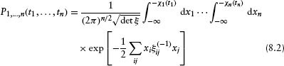
where the sum goes over i, j = 1,…, n, and ξ_ij^(–1) is the inverse of the n × n correlation matrix ξ_ij. For n not too large the integrals in equation 8.2 can be done numerically or, since defaults are rare, analytic results can be obtained using the leading terms in an asymptotic expansion of the integrals. The choice of a multivariate normal copula function is common but somewhat arbitrary. In principle, the copula function should be chosen based on a comparison with data. For recent work along these lines, see Das and Geng (2002).

In equation 8.2, the n × n correlation matrix ξ_ij is usually taken to be the asset correlation matrix. This has the advantage of allowing a connection to stock prices (Merton, 1974). However, this assumption is not necessary. For example, the assets, â_i could be functions of normal random variables, â_i = g_i(). Suppose default occurs if the assets â_i cross the thresholds T_i. Then, the condition for default on the normal production factor variables is that they cross the thresholds g_i^(–1) (T_i). In such a model it is natural to interpret ξ_ij as the correlation matrix for the normal production factor variables . If the functions g_i are linear, then the assets are also normal and their correlation matrix is also given by ξ_ij. However, if the functions g_i are not linear, the joint probability distribution for the assets is not multivariate normal and can have fat tails. Unless the g_i are specified, it is not possible to connect stock prices to the correlation matrix ξ_ij and the default thresholds χ_i. However, even when the functions g_i are not known, the default thresholds or “equivalent distances to default” χ_i(t_i) and the correlation matrix ξ_ij are determined by the default probabilities P_i(t_i) and the default correlations d_ij(t), and so have a direct connection to measures that investors use in quantifying security risk. In our work we assume that the correlation matrix is time-independent.

Equation 8.2 in the case n = 1 gives

Hence, for an explicit choice for the time dependence of the default probabilities, the default thresholds are known. A simple (and frequently used) choice for the default probabilities is

where the hazard rates h_i are independent of time.

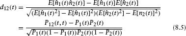
Since (t_i)² = (t_i) it follows that the correlation of defaults between two different firms(which we choose to label as 1 and 2) is

The default model we are adopting is not as well motivated as a first passagetime default model (Black and Cox, 1976; Longstaff and Schwartz, 1995; Leland and Toft, 1996, etc.) where the assets undergo a random walk, and default is associated with the first time the assets fall below the liabilities. However, it is very convenient to work with.

We will evaluate the integrals in equation 8.2 by numerical integration. For this we need the inverse and determinant of the correlation matrix. It is very important that the correlation matrix ξ_ij be positive semi-definite. If it has negative eigenvalues the integrals in equation 8.2 are not well defined. Typically, a correlation matrix that is forecast using qualitative methods will not be mathematically consistent and will have some negative eigenvalues. A practical method for constructing the consistent correlation matrix that is closest to a forecast one is given in Rebonato and Jäckel (2000). For the portfolios discussed in Sections 4 and 5, the n × n correlation matrix ξ_ij is taken to have all of its off-diagonal elements the same, that is, ξ_ij = ξ for i ≠ j. Such a correlation matrix has one eigenvalue equal to 1 + (n – 1)ξ and the others equal to 1 – ξ. Consequently, its determinant is

Its inverse has diagonal elements,

and off-diagonal elements(i ≠ j),

In the next section we consider the problem of portfolio allocation for portfolios consisting of corporate bonds subject to default risk and risk-free assets. The implications of default risk are addressed using the model discussed in this section. Other sources of risk—for example, systematic risk associated with the liquidity part of the excess risk premium—are neglected.

3. THE PORTFOLIO PROBLEM

Assume a zero-coupon bond from company i grows in value (if it does not default) at the (short) corporate rate c_i(t) and that if the company defaults, a fraction R_i of the value of that bond at the time of default is reinvested at the risk-free (short) rate y(t). Then, the random variable for the value of this bond at some time T in the future is

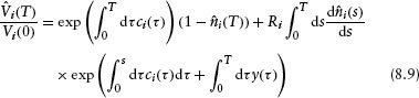
where V_i(0) is the initial value of the zero-coupon bond. In equation 8.9 we have continuously compounded the returns and we have assumed that T is less than or equal to the maturity date of the bond.⁵ Note that the random variable d(t)/dt is equal to the Dirac delta function, δ(t – t_i), if company i defaults at the time t_i and is zero if it does not default. The first term in equation 8.9 gives the value if the company does not default before time T and the second term (proportional to R_i) gives the value if the company defaults before time T. The corresponding formula for a risk-free asset is

Note that we are not treating the (short) risk-free rate y(τ) as a random variable, although it is certainly possible to generalize this formalism to do that. The (short) corporate rate is decomposed as

where μ_i is the excess risk premium and λ_i is the part of the corporate short rate that compensates the investor in an actuarially fair way for the fact that the value of the investment can be reduced through corporate default. In other words,

Taking the expected value, equation 8.12 implies that

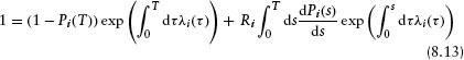
Differentiation with respect to T gives

Using equation 8.4 for the time dependence of the probabilities of default, equation 8.14 implies the familiar relation

The above results imply that the total wealth, after time T, in a portfolio consisting of risk-free assets and zero-coupon corporate bonds that are subject to default risk is (assuming the bonds mature at dates greater than or equal to T)

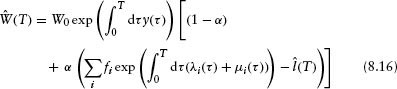
where W₀ is the initial wealth, α the fraction of corporate assets in the portfolio, (T) the random variable for the fractional default loss over the time period T, R_i the recovery fraction, and f_i denotes the initial fraction of corporate assets in the portfolio that are in firm i (Σ_i f_i = 1). In equation 8.16 the sum over i goes over all N firms in the portfolio and the default loss random variable is given by

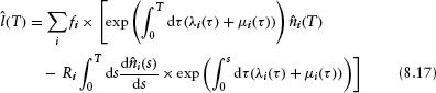
Integrating by parts,

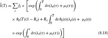
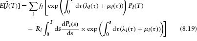
The expected value of (T) is

Fluctuations of the fractional loss (T) about its average value are described by the variable

The mean of δ is zero and the probability distribution for δ determines the default risk of the portfolio associated with fluctuations of the random variables (t). The moments of this probability distribution are

Using equation 8.1 and the property (t₁)(t₂) = (min[t₁,t₂]), the moments v^(m)(T) can be expressed in terms of the joint default probabilities.

The random variable for the portfolio wealth at time T is

where

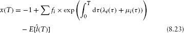
Using equations 8.13 and 8.19 we find that

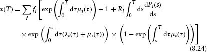
Note that x(T) vanishes if the excess risk premiums μ_i do.

To find out what value of α is optimal for some time horizon T, a utility function is introduced that characterizes the investor's level of risk aversion. Here, we use utility functions of the type U_γ (W) = W^γ/γ that have constant relative risk aversion,⁶ 1 – γ. The optimal fraction of corporates, α_opt, maximizes the expected utility of wealth E[U_γ((T))]. Expanding the utility of wealth in a power series in δ and taking the expected value gives

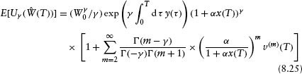
where Γ is the Euler Gamma function. The approximate optimal value of α obtained from truncating the sum in equation 8.25 at the mth moment is denoted by α_m. The focus of this chapter is on portfolios that are not leveraged and have α_opt less than unity. We will later see that typically for such portfolios, the α_m converge very quickly to α_opt so that for practical purposes only a few of the moments v^(m) need to be calculated. Note that the value of α_opt is independent of the risk-free rate y(t).

The expressions for (T) and x(T) are complicated but they do simplify for short times T or if all the recovery fractions are zero. For example, if T is small

and

On the other hand, if all the recovery fractions vanish (i.e., R_i = 0), then,

and

If x(T) is zero, then α_opt is also zero. It is x(T) that contains the dependence on the excess risk premiums that provide the incentive for a risk-adverse investor to choose corporate bonds over risk-free assets. An approximate formula for α_opt can be derived by expanding it in x(T):

The coefficients s_i(T) can be expressed in terms of the moments, v^(m)(T). Explicitly, for the first two coeffcients,

and

For γ < 1, including the third moment reduces the optimal fraction of corporates when v⁽³⁾(T) is positive.

4. SAMPLE PORTFOLIOS WITH ZERO RECOVERY FRACTIONS

Here, we consider very simple sample portfolios where the correlations, default thresholds, and excess risk premiums are the same for all N firms in the portfolio, that is, ξ_ij = ξ, χi(t) = χ(t) and μ_i(t) = μ⁷. Then, all the probabilities of default are the same, P_i(t) = P(t), and the joint default probabilities are also independent of which firms are being considered, P_i1,…,i_m(t₁,…, t_m) = P₁₂,…,m(t₁,…, t_m). The time dependence of the default probabilities is taken to be given by equation 8.4. Given our assumptions, the hazard rates are then also independent of firm, h_i = h. We also take the portfolios to contain equal assets in the firms so that f_i = 1/N, for all i, and assume all the recovery fractions are zero. Since the portfolio allocation problem does not depend on the risk-free rate y or the initial wealth, we set y = 0 and W₀ = 1.

With these assumptions the expressions for (T) and x(T) become

and

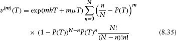
For random defaults, the probability of a fractional loss of = exp(hT + μT)n/N in the time horizon T is (1 – P(T))^N–nP(T)ⁿN!/(N – n)!n! and so the mth moment of the default loss distribution is

The expected utility of wealth is

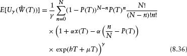
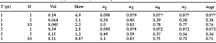
Having the explicit expression for the utility of wealth in equation 8.36, let us compare results of the moment expansion for the optimal fraction of corporates α_m with the all-orders result, α_opt. These are presented in Table 8.1 in the case h = 0.02, μ = 100 bp, and γ = −4. Results for different values of the number of firms N and different time horizons T are shown in Table 8.1. We also give in columns three and four of Table 8.1 the volatility

Table 8.1 Optimal Fraction of Corporates for Sample Portfolios with Random (ξ = 0) Defaults. Other Parameters Used Are h = 0.02, γ = −4, and μ = 100 bp

and skewness

of the portfolio default loss probability distribution.

Increasing N gives a larger value for the optimal fraction of corporates because diversification reduces risk. This occurs very rapidly with N. For N = 1, μ = 100 bp, T = 1yr, and γ = −4 the optimal fraction of corporates is only 7.7%. By N = 10, increasing the number of firms has reduced the portfolio default risk so much that the 100 bp excess risk premium causes a portfolio that is 76% corporates to be preferred.

For all the entries in Table 8.1 the moment expansion converges very rapidly, although for low N it is the small value of α_opt that is driving the convergence. Since in equation 8.25 the term proportional to v^(m) has a factor of α^m accompanying it, we expect good convergence of the moment expansion at small α.

The focus of this chapter is on portfolios that are not leveraged and have α_opt < 1. But a value α_opt > 1 is not forbidden when finding the maximum of the expected utility of wealth. This occurs at lowest order in the moment expansion in the last row of Table 8.1.

Next we consider the more typical case where there are correlations, ξ ≠ 0. Table 8.2 gives values of α₂-α₅ for T = 1yr, μ = 100 bp, h = 0.02, and γ = −4. Portfolios with N = 10, 50, and 100 are considered and values for ξ between 0.5 and 0.25 are used.

Again, the convergence of the moment expansion is quite good. Although just including the variance (i.e., α₂) can be off by a factor of almost two, α₃ is usually a reasonable approximation to the true optimal fraction of corporates. The convergence is worse, the larger the value of α_opt; for values of α_opt less than 40% we find that α₃ is within about 10% of α_opt.

In the last row of Table 8.2 the value of α₅ is equal to unity. However, we know that the true value of α_opt must be less than unity. For α = 1 there is some finite (but tiny) chance of investors losing all their wealth and for γ < 0, the utility of zero wealth is –∞.

Table 8.2 Moment Expansion for Optimal Portfolio with Correlated Defaults for T = 1 Yr, μ = 100 bp, h = 0.02, and γ = −4

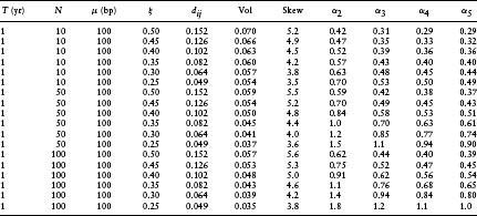
Correlations dramatically affect the dependence of the optimal portfolio allocation on the total number of firms. For the ξ = 0.5 entries in Table 8.2, the optimal fraction of corporates is 0.29, 0.37, and 0.39 for N = 10, 50, and 100, respectively. For N = 10,000 we find that α₅ = 0.40. Increasing the number of firms beyond 100 only results in a small increase in the optimal fraction of corporates. When defaults are random the moments of the portfolio default loss distribution go to zero as N → ∞. For example, with ξ = 0, the variance of the default loss distribution is

and the skewness of the default loss distribution is

For random defaults, as N → ∞, the distribution for δ approaches the trivial one where δ = 0 occurs with unit probability. However, for ξ < 0 the moments v^(m) go to nonzero values in the limit N → ∞ and the default loss distribution remains nontrivial and non-normal.

In Table 8.3 the time horizon is changed to T = 5 yr but the other parameters are the same as in Table 8.2. The value of α_opt is always smaller than in Table 8.2, indicating that the compounding of the excess risk premium does not completely compensate for the added risk associated with the greater probability of default. The convergence of the moment expansion and the

Table 8.3 Moment Expansion for Optimal Portfolio with Correlated Defaults for T = 5 Yr, μ = 100 bp, h = 0.02, and γ = −4

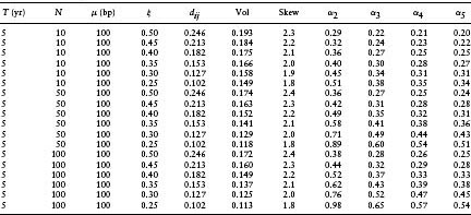
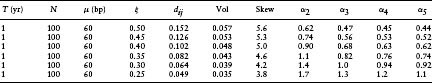
Table 8.4 Moment Expansion for Optimal Portfolio with Correlated Defaults for T = 1Yr, N = 100, μ = 60 bp, h = 0.02, and γ = −2

dependence of the optimal fraction of corporates on the number of bonds is similar to that in Table 8.2.

Table 8.3 indicates that the volatility of the portfolio default loss probability distribution increases as the time horizon increases, and the skewness decreases as the time horizon increases. The same behavior occurs for random defaults and this can be seen from equations 8.39 and 8.40 with the small probability of default P increasing with time.

Next we consider the effect of changing the utility function to one with a lower level of risk aversion. In Table 8.4, γ = −2 is used. Equation 8.31 suggests that an excess risk premium of 60 bp would yield roughly the same portfolio allocation as the excess risk premium of 100 bp used in Tables 8.2 and 8.3. In Table 8.4 we consider portfolios with 100 firms and take the same parameters as in Table 8.2 apart from the lower level of risk aversion, γ = −2, and the lower excess risk premium, μ = 60 bp.

It is not surprising that the values of α₂ in Table 8.4 are close to those in Table 8.2. However, α₅ is typically about 10% larger than in Table 8.2. The convergence of the moment expansion is better in Table 8.4 than in Table 8.2.

Table 8.5 Probability of Default and Convergence of the Moment Expansion for T = 1 Yr, ξ = 0.50, N = 100, and γ = −4

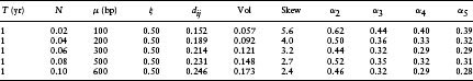
The examples in this section have all used an annualized hazard rate of 2%; however, the convergence of the moment expansion is similar for significantly larger default probabilities. In Table 8.5 the convergence of the moment expansion is examined for portfolios with 100 corporate bonds and hazard rates of 2, 4, 6, 8, and 10%. The value of ξ is fixed at 0.50 and the time horizon is 1 year. The convergence of the moment expansion is good for all the values of h used in Table 8.5.

For longer time horizons the increased default risk is not compensated for by the compounding of the excess risk premium. For example, if we take the parameters of the last row of Table 8.5 but increase the time horizon to T = 5 years, then α₂ = 0.25, α₃ = 0.21, α₄ = 0.18, and α₅ = 0.17.

5. SAMPLE PORTFOLIOS WITH NONZERO RECOVERY FRACTIONS

In this section we consider portfolios like those in Section 4 but allow the recovery fractions R_i = R to be nonzero. Here, we focus on short time horizons using the approximate formulas,

and

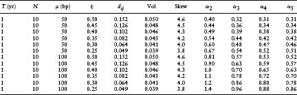
appropriate to that regime. Recall that if R is not zero the actuarially fair corporate spread is λ = h(1 – R). Table 8.6 shows the impact of nonzero recovery on α_opt. The parameters used are γ = −4, T = 1year, N = 10, R = 0.5, h = 0.04, and μ = 50 and 100 bp. Doubling the hazard rate to 0.04 gives an actuarially fair corporate spread of 200 bp, which is the same as in Tables 8.2 and 8.3. Note that even though the actuarially fair spread in Table 8.6 is the same as in Table 8.2, nonzero recovery reduces the default risk and so the excess risk premium must be reduced by a factor of 2 to get values of α_opt close to those in Table 8.2.

Table 8.6 Recovery and Moment Expansion for Optimal Portfolio with Correlated Defaults Using T = 1 Yr, N = 10, h = 0.04, R = 0.5, and γ = −4

For random defaults one can easily see why recovery reduces portfolio default risk. Taking the hazard rate to be small, the time horizon to be short, and the defaults to be random,

and

where λ is the actuarially fair spread. Hence, with λ held fixed, the variance and skewness of the portfolio default loss probability distribution decrease as R increases

Since we are using the approximate formulas in equations 8.41 and 8.42, we would not get exact agreement with Table 8.2 even if R = 0. For example, with T = 1 year, N = 10, γ = −4, μ = 100 bp, h = 0.02, ξ= 0.5, and R = 0, using equations 8.41 and 8.42 yields α₂ = 0.44, α₃ = 0.33, α₄ = 0.31, and α₅ = 0.30. On the other hand, the first row of Table 8.2 is α₂ = 0.42, α₃ = 0.31, α₄ = 0.29, and α₅ = 0.29.

6. CONCLUDING REMARKS

Default correlations have an important impact on portfolio default risk. Given a default model, the tail of the default loss probability distribution is difficult to compute, often involving numerical simulation⁸ of rare events. The first few moments of the default loss distribution are easier to calculate, and in the default model we used, this computation involved some simple numerical integration. More significantly, the first few terms in the moment expansion have a familiar meaning. Investors are used to working with the classic mean, variance, and skewness measures and have developed intuition for them and confidence in them. In this chapter, we studied the utility of the first few moments of the default loss probability distribution for the portfolio allocation problem.

The default model we use assumes a multivariate normal copula function. However, the corporate assets themselves are not necessarily normal or lognormal and their probability distribution can have fat tails. When there are correlations, the portfolio default loss distribution does not approach a trivial⁹ or normal probability distribution as the number of firms in the portfolio goes to infinity. Correlations dramatically decrease the effectiveness of increasing the number of firms, N, in the portfolio to reduce portfolio default risk.

We explored the convergence of the moment expansion for the optimal fraction of corporate assets α_opt. Our work indicates that, for α_opt less than unity, the convergence of the moment expansion is quite good. The convergence of the moment expansion gets poorer as α_opt gets larger. We also examined how α_opt depends on the level of risk aversion, the recovery fraction, and investment time horizon.

The value of α_opt depends on the utility function used. In this chapter, we used utility functions with constant relative risk aversion, 1 – γ. It is possible to make other choices and whereas the quantitative results will be different for most practical purposes, we expect that the general qualitative results should continue to hold.

Our main conclusions from the examples in Sections 4 and 5 are as follows:

• In the presence of correlated defaults, the default loss distribution is not normal. Nevertheless, we find that retaining just the first few moments of the default loss probability distribution yields a good estimate of the optimal fraction of corporates. As α_opt gets smaller, the convergence of the moment expansion improves. For the examples in Sections 4 and 5 with α_opt near 40%, retaining just the mean, variance, and skewness of the default loss probability distribution determined α_opt with a precision better than about 15%.
• For small numbers of corporate bonds, increasing the number of firms decreases portfolio default risk. However, correlations cause this effect to saturate as the number of bonds increases. For the examples in Sections 4 and 5 (with production factor or asset correlations 0.50 ≥ ξ ≥ 0.25), the optimal fraction of corporates does not increase significantly if N is increased beyond 100 firms.
• Increasing the recovery fractions decreases portfolio risk and this is true even when the probabilities of default increase so that the actuarially fair spreads remain constant.
• With probabilities of default given by P_i(T) = 1 – exp(–h_iT) and the hazard rates h_i constant, continuous compounding of a constant excess risk premium does not exactly compensate for the increase in the default probability with time. The optimal fraction of corporates decreased in going from a T = 1-year to a T = 5-year investment horizon.

ACKNOWLEDGMENTS

The authors would like to thank their colleagues at PIMCO for enlightening discussions. Mark B. Wise was supported in part by the Department of Energy under contract DE-FG03-92-ER40701.

NOTES

1. In this chapter, we use annualized units, so quoted default probabilities, hazard rates, and corporate rates are annualized ones.

2. The authors would like to thank David Hinman of PIMCO for enlightening discussions on this topic.

3. See, for example, Jorion (2001).

4. Zhou (2001) derives an analytic formula for default correlations in a first passage-time default model and finds a similar increase with time horizon.

5. Assuming that after maturity the value of a zero-coupon corporate bond is reinvested at the risk-free rate. It is straightforward to generalize the analysis of this chapter to portfolios containing zero-coupon bonds with different maturities, some of which are less than the investment horizon. Similarly, default risk for portfolios containing coupon-paying bonds can be studied since each coupon payment can be viewed as a zero-coupon bond.

6. See, for example, Ingersoll (1987).

7. We also assume that μ is independent of time.

8. See, for example, Duffie and Singleton (1999) and Das et al. (2001).

9. The trivial distribution has δ = 0 occuring with unit probability.

REFERENCES

Altman, E. I. (1989). “Measuring Corporate Bond Mortality and Performance.” Journal of Finance 44(4), 909–921.

Black, F. and Cox, J. (1976). “Valuing Corporate Securities: Some Effects of Bond Indenture Provisions.” Journal of Finance 31, 351–367.

Das, S., Fong, G. and Geng, G. (2001). “The Impact of Correlated Default Risk on Credit Portfolios.” Working Paper, Department of Finance, Santa Clara University and Gifford Fong Associates.

Das, S., Freed, L., Geng, G. and Kapadia, N. (2001). “Correlated Default Risk.” Working Paper, Department of Finance, Santa Clara University and Gifford Fong Associates.

Das, S. and Geng, G. (2002). “Modeling the Process of Correlated Default.” Working Paper, Department of Finance, Santa Clara University and Gifford Fong Associates.

Duffie, D. and Singleton, K. (1999). “Simulating Correlated Defaults.” Working Paper, Stanford University Graduate School of Business.

Dynkin, L., Hyman, J. and Konstantinovsky, V. (2002). “Sufficient Diversification in Credit Portfolios.” Lehman Brothers Fixed Income Research (working paper).

Ingersoll, J. (1987). Theory of Financial Decision Making. Lanham, MD: Rowman and Littlefield Publishers Inc.

Jorion, P. (2001). Value at Risk, 2nd edn. New York: McGraw-Hill Inc.

Li, D. (2000). “On Default Correlation: A Copula Function Approach.” Working Paper 99–07, The Risk Metrics Group.

Leland, H. and Toft, K. (1996). “Optimal Capital Structure, Endogenous Bankruptcy and the Term Structure of Credit Spreads.” Journal of Finance 51, 987–1019.

Longstaff, F. and Schwartz, E. (1995). “A Simple Approach to Valuing Risky Floating Rate Debt.” Journal of Finance 50, 789–819.

Lucas, D. (1995). “Default Correlation and Credit Analysis.” Journal of Fixed Income, 4(4), 76–87.

Merton, R. (1974). “On Pricing of Corporate Debt: The Risk Structure of Interest Rates.” Journal of Finance 29, 449–470.

Rebonato, R. and Jackel, P. (2000). “The Most General Methodology for Creating a Valid Correlation Matrix for Risk Management and Option Pricing Purposes.” The Journal of Risk 2(2), 17–26.

Wise, M. and Bhansali, V. (2002). “Portfolio Allocation to Corporate Bonds with Correlated Defaults.” Journal of Risk 5(1), Fall.

Zhou, C. (2001). “An Analysis of Default Correlations and Multiple Defaults.” The Review of Financial Studies 12(2), 555–576.

Keywords: Asset correlations; default; corporate bonds; portfolio allocation

---

^aCalifornia Institute of Technology, Pasadena CA 91125, USA.

^bPIMCO, 840 Newport Center Drive, Suite 300, Newport Beach, CA 92660, USA.

^*Corresponding author. California Institute of Technology, Pasadena CA 91125, USA. E-mail: [email protected].