There is a tongue-in-cheek statement attributed to an unknown Twitter user: “If a MongoDB query runs for longer than 0ms, then something is wrong.” This is typical of the kind of buzz that surrounded the product when it first burst onto the scene in 2009.

The reality is that MongoDB is extraordinarily fast. But if you give it the wrong data structures, or you don’t set up collections with the right indexes, MongoDB can slow down dramatically, like any data storage system. MongoDB also contains advanced features, which require some tuning to get them running with optimal efficiency.

The design of your data schemas can also have a big impact on performance; in this chapter, we will look at some techniques to shape your data into a form that makes maximum use of MongoDB’s strengths and minimizes its weaknesses.

Before we look at improving the performance of the queries being run on the server or the ways of optimizing the structure of the data, we’ll begin with a look at how MongoDB interacts with the hardware it runs on and the factors that affect performance. We then look at indexes and how they can be used to improve the performance of your queries and how to profile your MongoDB instance to determine which, if any, of your queries are not performing well.

Optimizing Your Server Hardware for Performance

Often the quickest and least expensive optimizations you can make to a database server is to right-size the hardware it runs on. If a database server has too little memory or uses slow drives, it can impact database performance significantly. And while some of these constraints may be acceptable for a development environment, where the server may be running on a developer’s local workstation, they may not be acceptable for production applications, where care must be used in calculating the correct hardware configuration to achieve the best performance.

Understanding MongoDB’s Storage Engines

By far the largest change in recent history to MongoDB is the addition of the new storage engine’s API. With this API there have also been several storage engines released, and among these, the headliner is the much talked about WiredTiger. As of MongoDB 3.0, you can specify which storage engine you wish to use with the –storageEngine command-line option or the storage.engine YAML option. The original (and prior to MongoDB 3.0, only) storage engine was called MMAPv1. The WiredTiger storage engine, first available as part of the 3.0 release, is now the default storage engine as of MongoDB 3.2.

Probably the most important thing to be aware of when thinking about storage engines is that once you first start a MongoDB instance, the storage engine is fixed. It is possible to change storage engines by dumping all of the data in your system, deleting the database content, and reimporting the data once more, but as you can imagine, this is a tiring and long process. This makes selecting up front the right storage engine for the job important. For the most part you will be best served by using the default storage engine in MongoDB 3.2, which is WiredTiger.

WiredTiger offers a number of improvements over the previous MMAPv1 storage engine. WiredTiger has an internal MVCC (multi-version concurrency control) model that allows MongoDB to fully support document-level locking, which is a big improvement over the collection-level locking found in MMAPv1. WiredTiger also takes responsibility for all memory management involved with your data, rather than delegating to the operating system’s kernel as MMAPv1 did. Various benchmarks from both the MongoDB team and other users of MongoDB on the Internet have shown that under most circumstances WiredTiger is the better choice of storage engine. In addition to this, WiredTiger provides the ability to compress all your data automatically using one of several compression algorithms. These provide a large savings to the amount of storage space needed for your data.

Understanding MongoDB Memory Use Under MMAPv1

MongoDB’s MMAPv1 storage engine used memory-mapped file I/O to access its underlying data storage. This method of file I/O has some characteristics that you should be aware of, because they can affect both the type of operating system (OS) you run it under and the amount of memory you install.

The first notable characteristic of memory-mapped files is that, on modern 64-bit operating systems, the maximum file size that can be managed is around 128TB on Linux (the Linux virtual memory address limit) or 8TB (4TB with Journaling enabled) on Windows because of its limitation for memory-mapped files. On 32-bit operating systems, you are limited to only 2GB worth of data, so it is not recommended that you use a 32-bit OS unless you are running a small development environment.

The second notable characteristic is that memory-mapped files use the operating system’s virtual memory system to map the required parts of the database files into RAM as needed. This can result in the slightly alarming impression that MongoDB is using up all your system’s RAM. That is not really the case, because MongoDB will share the virtual address space with other applications. And the OS will release memory to the other processes as it is needed. Using the free memory total as an indicator of excessive memory consumption is not a good practice, because a good OS will ensure that there is little or no “free” memory. All of your expensive memory is pressed into good use through caching or buffering disk I/O. Free memory is wasted memory.

By providing a suitable amount of memory, MongoDB can keep more of the data it needs mapped into memory, which reduces the need for expensive disk I/O.

In general, the more memory you give to MongoDB, the faster it will run. However, if you have a 2GB database, then adding more than 2 to 3GB of memory will not make much difference, because the whole database will sit in RAM anyway.

Understanding Working Set Size in MMAPv1

We also need to explain one of the more complex things involved with performance tuning your MongoDB MMAPv1 instance: working set size. This size represents the amount of data stored in your MongoDB instance that will be accessed “in the course of regular usage.” That phrase alone should tell you that this is a subjective measure and something that is hard to get an exact value for.

Despite being hard to quantify, understanding the impact of working set size will help you better optimize your MongoDB instance. The main precept is that for most installations, only a portion of the data will need to be accessed as part of regular operations. Understanding what portion of your data you will be working with regularly allows you to size your hardware correctly and thus improves your performance.

Understanding MongoDB Memory Use Under WiredTiger

As mentioned earlier, WiredTiger uses a memory model that works to keep as much of the “relevant” data in memory at a given time. Relevant in this context is the data that are needed right now in order to fulfill the operations that are being worked on within your system currently. In MongoDB terms, this memory space where documents are stored in memory is called the cache. By default, MongoDB will reserve roughly half of the available system memory for use in storing these documents. This value can be tuned with the wiredTigerCacheSizeGB command-line option or the storage.wiredTiger.engineConfig.cacheSizeGB YAML configuration option.

In almost all cases the default cache size is more than adequate for most systems, and changes to this value are normally found to be detrimental; however, if you have a dedicated server with plenty of memory, you can test (and test thoroughly) running with a higher cache size. But be warned, this is only the amount of memory that will be used for storing documents; all of the memory used in maintaining connections, running database internals, and performing user operations are counted elsewhere, so you should never look to allocate 100% of your system memory to MongoDB or else you will begin to see the database process being killed by your OS!

Compression in WiredTiger

WiredTiger supports compression of your data on disk. There are three places within your data storage that WiredTiger can compress your data and there are two compression algorithms you can use with your data that have slightly different trade-offs:

• The first and default compression algorithm is the snappy compression algorithm. This compression algorithm provides good compression and has really low overhead in terms of CPU usage.
• The second algorithm is the zlib compression algorithm. This algorithm provides very high compression but costs significantly more in terms of CPU and time.
• The third and final compression available within MongoDB is the none compression algorithm, which simply disables compression.

Now that we have covered the compression algorithms, we can look at which MongoDB data you can compress:

• Data in your collections.
• Index data, which are the data in your indexes.
• Journal data, which is that used to ensure your data are redundant and recoverable while they are being written into your long-term data storage.

Finally, armed with a sense of understanding of what compression can be used on which data, let’s look at how you can compress things. It’s important to note that these options are set in your MongoDB configs when you boot up your instance and will affect only new data objects when created. Any existing objects will continue to use the compression they were created with. For example, if you create a collection with the default snappy compression algorithm and then decide you wish to use the zlib compression algorithm for your collections, your existing collections will not switch to snappy but any new collections will be made with zlib. The setting of compression algorithms is done with three different YAML configuration settings that take either snappy, zlib, or none as the values:

• For Journal compression you use the storage.wiredTiger.engineConfig.journalCompressor YAML configuration option, which takes a value of the name of the compression lib you wish to use.
• For Index compression you use the storage.wiredTiger.indexConfig.prefixCompression YAML configuration option, which takes a true or false value to say if index prefix compression should be on or off. This is on by default.
• For Collection compression you use the storage.wiredTiger.collectionConfig.blockCompressor YAML configuration option, which takes a value of the name of the compression lib you wish to use.

With these options you should be able to configure the compression in your system to best suit your needs.

Choosing the Right Database Server Hardware

There is often an overall pressure to move to lower-power (energy) systems for hosting services. However, many of the lower-power servers use laptop or notebook components to achieve the lower-power consumption. Unfortunately, lower-quality server hardware often uses less-expensive disk drives in particular. Such drives are not suited for heavy-duty server applications because of their disks’ low rotation speed, which slows the rate at which data can be transferred to and from the drive. Also, make sure you use a reputable supplier, one you trust to assemble a system that has been optimized for server operation. It’s also worth mentioning that faster and more modern drives such as SSDs are available, which will provide a significant performance boost. If you can arrange it, the MongoDB, Inc. team recommends the use of RAID10 for both performance and redundancy. For those of you in the cloud, getting something like Provisioned IOPS from Amazon is a great way to improve the performance and reliability of your disks.

If you plan to use replication or any kind of frequent backup system that would have to read across the network connections, you should consider putting in an extra network card and forming a separate network so the servers can talk with each other. This reduces the amount of data being transmitted and received on the network interface used to connect the application to the server, which also affects an application’s performance.

Probably the biggest thing to be aware of when purchasing hardware is RAM. Having sufficient space to keep necessary data somewhere that it can be accessed quickly is a great way to ensure high performance. Having an idea of how much memory you need to allocate for a given amount of data is the key when looking to purchase hardware. Finally, remember that you don’t need to buy 512GB of RAM and install it on one server; you can spread the data load out using sharding (discussed in Chapter 12).

Evaluating Query Performance

MongoDB has two main tools for optimizing query performance: explain() and the MongoDB Profiler (hereafter the profiler). The profiler is a good tool for locating the queries that are not performing well and selecting candidate queries for further inspection, while explain() is good for investigating a single query, so you can determine how well it is performing.

Those of you who are familiar with MySQL will probably also be familiar with the use of the slow query log, which helps you find queries that are consuming a lot of time. MongoDB uses the profiler to provide this capability. In addition to this, MongoDB will always write out queries that take longer than a certain time (by default 100ms) to the logfile. This 100ms default can be changed by setting the slowMS value, as we will cover below.

The MongoDB Profiler

The MongoDB profiler is a tool that records statistical information and execution plan details for every query that meets the current profiling level criteria. You can enable this tool separately on each database or for all databases by using the --profile and --slowms options to start your MongoDB process (more on what these values mean shortly). These options can also be added to your mongod.conf file, if that is how you are starting your MongoDB process.

Once the profiler is enabled, MongoDB inserts a document with information about the performance and execution details of each query submitted by your application into a special capped collection called system.profile. You can use this collection to inspect the details of each query logged using standard collection querying commands.

The system.profile collection is limited to a maximum of 1024KB of data, so that the profiler will not fill the disk with logging information. This limit should be enough to capture a few thousand profiles of even the most complex queries.

Enabling and Disabling the MongoDB Profiler

It’s a simple matter to turn on the MongoDB profiler:

$mongo
>use blog
>db.setProfilingLevel(1)

It is an equally simple matter to disable the profiler:

$mongo
>use blog
>db.setProfilingLevel(0)

MongoDB can also enable the profiler only for queries that exceed a specified execution time. The following example logs only queries that take more than half a second to execute:

$mongo
>use blog
>db.setProfilingLevel(1,500)

As shown here, for profiling level 1, you can supply a maximum query execution time value in milliseconds (ms). If the query runs for longer than this amount of time, it is profiled and logged; otherwise, it is ignored. This provides the same functionality seen in MySQL’s slow query log.

Finally, you can enable profiling for all queries by setting the profiler level to 2.

$mongo
>use blog
>db.setProfilingLevel(2)

Finding Slow Queries

A typical document in the system.profile collection looks like this:

> db.system.profile.find()
{
        "op" : "query",
        "ns" : "blog.blog.system.profile",
        "query" : {
                "find" : "blog.system.profile",
                "filter" : {

                }
        },
        "keysExamined" : 0,
        "docsExamined" : 0,
        "cursorExhausted" : true,
        "keyUpdates" : 0,
        "writeConflicts" : 0,
        "numYield" : 0,
        "locks" : {
                "Global" : {
                        "acquireCount" : {
                                "r" : NumberLong(2)
                        }
                },
                "Database" : {
                        "acquireCount" : {
                                "r" : NumberLong(1)
                        }
                },
                "Collection" : {
                        "acquireCount" : {
                                "r" : NumberLong(1)
                        }
                }
        },
        "nreturned" : 0,
        "responseLength" : 115,
        "protocol" : "op_command",
        "millis" : 12,
        "execStats" : {
                "stage" : "EOF",
                "nReturned" : 0,
                "executionTimeMillisEstimate" : 0,
                "works" : 0,
                "advanced" : 0,
                "needTime" : 0,
                "needYield" : 0,
                "saveState" : 0,
                "restoreState" : 0,
                "isEOF" : 1,
                "invalidates" : 0
        },
        "ts" : ISODate("2015-10-20T09:52:26.477Z"),
        "client" : "127.0.0.1",
        "allUsers" : [ ],
        "user" : ""
}

Each document contains fields, and the following list outlines what they are and what they do:

• op: Displays the type of operation; it can be either query, insert, update, command, or delete.
• query: The query being run.
• ns: The full namespace this query was run against.
• ntoreturn: The number of documents to return.
• nscanned: The number of index entries scanned to return this document.
• ntoskip: The number of documents skipped.
• keyUpdates: The number of index keys updated by this query.
• numYields: The number of times this query yielded its lock to another query.
• lockStats: The number of microseconds spent acquiring or in the read and write locks for this database.
• nreturned: The number of documents returned.
• responseLength: The length in bytes of the response.
• millis: The number of milliseconds it took to execute the query.
• ts: Displays a timestamp in UTC that indicates when the query was executed.
• client: The connection details of the client who ran this query.
• user: The user who ran this operation.

Because the system.profile collection is just a normal collection, you can use MongoDB’s query tools to zero in quickly on problematic queries.

The next example finds all the queries that are taking longer than 10ms to execute. In this case, you can just query for cases where millis >10 in the system.profile collection, and then sort the results by the execution time in descending order:

> db.system.profile.find({millis:{$gt:10}}).sort({millis:-1})
{ "op" : "query", "ns" : "blog.blog.system.profile", "query" : { "find" : "blog.system.profile", "filter" : {  } }, "keysExamined" : 0, "docsExamined" : 0, "cursorExhausted" : true, "keyUpdates" : 0, "writeConflicts" : 0, "numYield" : 0, "locks" : { "Global" : { "acquireCount" : { "r" : NumberLong(2) } }, "Database" : { "acquireCount" : { "r" : NumberLong(1) } }, "Collection" : { "acquireCount" : { "r" : NumberLong(1) } } }, "nreturned" : 0, "responseLength" : 115, "protocol" : "op_command", "millis" : 12, "execStats" : { "stage" : "EOF", "nReturned" : 0, "executionTimeMillisEstimate" : 0, "works" : 0, "advanced" : 0, "needTime" : 0, "needYield" : 0, "saveState" : 0, "restoreState" : 0, "isEOF" : 1, "invalidates" : 0 }, "ts" : ISODate("2015-10-20T09:52:26.477Z"), "client" : "127.0.0.1", "allUsers" : [ ], "user" : "" }

If you also know your problem occurred during a specific time range, then you can use the ts field to add query terms that restrict the range to the required slice.

Increase the Size of Your Profile Collection

If you find that for whatever reason your profile collection is just too small, you can increase its size.

First, you need to disable profiling on the database whose profile collection size you wish to increase, to ensure that nothing writes to it while you are doing this operation:

$mongo
>use blog
>db.setProfilingLevel(0)

Next, you need to delete the existing system.profile collection:

>db.system.profile.drop()

With the collection dropped, you can now create your new profiler collection with the createCollection command and specify the desired size in bytes. The following example creates a collection capped at 50MB. It uses notation that converts 50 bytes into kilobytes and then into megabytes by multiplying it by 1024 for each increase in scale:

>db.createCollection( "system.profile", { capped: true, size: 50 * 1024 * 1024 } )
{ "ok" : 1 }

With your new larger capped collection in place, you can now re-enable profiling:

>db.setProfilingLevel(2)

Analyzing a Specific Query with explain()

If you suspect a query is not performing as well as expected, you can use the explain() modifier to see exactly how MongoDB is executing the query.

When you add the explain() modifier to a query, on execution MongoDB returns a document that describes how the query was handled, rather than a cursor to the results. The following query runs against a database of blog posts and indicates that the query had to scan 13,325 documents to form a cursor to return all the posts:

$mongo
>use blog
> db.posts.find().explain(true)
{
        "waitedMS" : NumberLong(0),
        "queryPlanner" : {
                "plannerVersion" : 1,
                "namespace" : "test.posts",
                "indexFilterSet" : false,
                "parsedQuery" : {
                        "$and" : [ ]
                },
                "winningPlan" : {
                        "stage" : "COLLSCAN",
                        "filter" : {
                                "$and" : [ ]
                        },
                        "direction" : "forward"
                },
                "rejectedPlans" : [ ]
        },
        "executionStats" : {
                "executionSuccess" : true,
                "nReturned" : 13325,
                "executionTimeMillis" : 3,
                "totalKeysExamined" : 0,
                "totalDocsExamined" : 13325,
                "executionStages" : {
                        "stage" : "COLLSCAN",
                        "filter" : {
                                "$and" : [ ]
                        },
                        "nReturned" : 13325,
                        "executionTimeMillisEstimate" : 10,
                        "works" : 13327,
                        "advanced" : 13325,
                        "needTime" : 1,
                        "needYield" : 0,
                        "saveState" : 104,
                        "restoreState" : 104,
                        "isEOF" : 1,
                        "invalidates" : 0,
                        "direction" : "forward",
                        "docsExamined" : 13325
                },
                "allPlansExecution" : [ ]
        },
        "serverInfo" : {
                "host" : "voxl",
                "port" : 27017,
                "version" : "3.2.0-rc1-75-gfb6ebe7",
                "gitVersion" : "fb6ebe75207c3221314ed318595489a838ef1db0"
        },
        "ok" : 1
}

You can see the fields returned by explain() listed in Table 10-1.

Using the Profiler and explain() to Optimize a Query

Now let’s walk through a real-world optimization scenario and look at how we can use MongoDB’s profiler and explain() tools to fix a problem with a real application.

The example discussed in this chapter is based on a small sample blog application. This database has a function to get the posts associated with a particular tag; in this case it’s the even tag. Let’s assume you have noticed that this function runs slowly, so you want to determine whether there is a problem.

Let’s begin by writing a little program to fill the aforementioned database with data so that you have something to run queries against to demonstrate the optimization process:

<?php

// Get a connection to the database

$mongo = new MongoClient();
$db=$mongo->blog;

// First let’s get the first AuthorsID
// We are going to use this to fake a author

$author = $db->authors->findOne();

if(!$author){
        die("There are no authors in the database");
}

for( $i = 1; $i < 10000; $i++){
        $blogpost=array();
        $blogpost[’author’] = $author[’_id’];
        $blogpost[’Title’]  = "Completely fake blogpost number {$i}";
        $blogpost[’Message’] = "Some fake text to create a database of blog posts";
        $blogpost[’Tags’] = array();
        if($i%2){
                // Odd numbered blogs
                $blogpost[’Tags’] = array("blog", "post", "odd", "tag{$i}");
        } else {
                // Even numbered blogs
                $blogpost[’Tags’] = array("blog", "post", "even", "tag{$i}");
        }
        $db->posts->insert($blogpost);
}
?>

This program finds the first author in the blog database’s authors collection, and then pretends that the author has been extraordinarily productive. It creates 10,000 fake blog postings in the author’s name, all in the blink of an eye. The posts are not very interesting to read; nevertheless, they are alternatively assigned odd and even tags. These tags will serve to demonstrate how to optimize a simple query.

The next step is to save the program as fastblogger.php and then run it using the command-line PHP tool:

$php fastblogger.php

Next, you need to enable the database profiler, which you will use to determine whether you can improve the example’s queries:

$ mongo
> use blog
switched to db blog
> show collections
authors
posts
...
system.profile
tagcloud
...
users
> db.setProfilingLevel(2)
{ "was" : 0, "slowms" : 100, "ok" : 1 }

Now wait a few moments for the command to take effect, open the required collections, and then perform its other tasks. Next, you want to simulate having the blog website access all of the blog posts with the even tag. Do so by executing a query that the site can use to implement this function:

$Mongo
use blog
$db.posts.find({Tags:"even"})
...

If you query the profiler collection for results that exceed 5ms, you should see something like this:

>db.system.profile.find({millis:{$gt:5}}).sort({millis:-1})
{ "op" : "query", "ns" : "blog.posts", "query" : { "tags" : "even" }, "ntoreturn" : 0, "ntoskip" : 0, "nscanned" : 19998, "keyUpdates" : 0, "numYield" : 0, "lockStats" : { "timeLockedMicros" : { "r" : NumberLong(12869), "w" : NumberLong(0) }, "timeAcquiringMicros" : { "r" : NumberLong(5), "w" : NumberLong(3) } }, "nreturned" : 0, "responseLength" : 20, "millis" : 12, "ts" : ISODate("2013-05-18T09:04:32.974Z"), "client" : "127.0.0.1", "allUsers" : [ ], "user" : "" }...

The results returned here show that some queries are taking longer than 0ms (remember the quote at the beginning of the chapter).

Next, you want to reconstruct the query for the first (and worst-performing) query, so you can see what is being returned. The preceding output indicates that the poorly performing query is querying blog.posts and that the query term is {Tags:"even"}. Finally, you can see that this query is taking a whopping 15ms to execute.

The reconstructed query looks like this:

>db.posts.find({Tags:"even"})
{ "_id" : ObjectId("4c727cbd91a01b2a14010000"), "author" : ObjectId("4c637ec8b8642fea02000000"), "Title" : "Completly fake blogpost number 2", "Message" : "Some fake text to create a database of blog posts", "Tags" : [ "blog", "post", "even", "tag2" ] }
{ "_id" : ObjectId("4c727cbd91a01b2a14030000"), "author" : ObjectId("4c637ec8b8642fea02000000"), "Title" : "Completly fake blogpost number 4", "Message" : "Some fake text to create a database of blog posts", "Tags" : [ "blog", "post", "even", "tag4" ] }
{ "_id" : ObjectId("4c727cbd91a01b2a14050000"), "author" : ObjectId("4c637ec8b8642fea02000000"), "Title" : "Completly fake blogpost number 6", "Message" : "Some fake text to create a database of blog posts", "Tags" : [ "blog", "post", "even", "tag6" ] }
...

This output should come as no surprise; this query was created for the express purpose of demonstrating how to find and fix a slow query.

The goal is to figure out how to make the query run faster, so use the explain() function to determine how MongoDB is performing this query:

> db.posts.find({Tags:"even"}).explain(true)
db.posts.find({Tags:"even"}).explain(true)
{
        "waitedMS" : NumberLong(0),
        "queryPlanner" : {
                "plannerVersion" : 1,
                "namespace" : "test.posts",
                "indexFilterSet" : false,
                "parsedQuery" : {
                        "Tags" : {
                                "$eq" : "even"
                        }
                },
                "winningPlan" : {
                        "stage" : "COLLSCAN",
                        "filter" : {
                                "Tags" : {
                                        "$eq" : "even"
                                }
                        },
                        "direction" : "forward"
                },
                "rejectedPlans" : [ ]
        },
        "executionStats" : {
                "executionSuccess" : true,
                "nReturned" : 14998,
                "executionTimeMillis" : 12,
                "totalKeysExamined" : 0,
                "totalDocsExamined" : 29997,
                "executionStages" : {
                        "stage" : "COLLSCAN",
                        "filter" : {
                                "Tags" : {
                                        "$eq" : "even"
                                }
                        },
                        "nReturned" : 14998,
                        "executionTimeMillisEstimate" : 10,
                        "works" : 29999,
                        "advanced" : 14998,
                        "needTime" : 15000,
                        "needYield" : 0,
                        "saveState" : 234,
                        "restoreState" : 234,
                        "isEOF" : 1,
                        "invalidates" : 0,
                        "direction" : "forward",
                        "docsExamined" : 29997
                },
                "allPlansExecution" : [ ]
        },
        "serverInfo" : {
                "host" : "voxl",
                "port" : 27017,
                "version" : "3.2.0-rc1-75-gfb6ebe7",
                "gitVersion" : "fb6ebe75207c3221314ed318595489a838ef1db0"
        },
        "ok" : 1
}

You can see from the output here, the query is not using any indexes as given by the winningPlan being COLLSCAN. Specifically, it’s scanning all the documents in the database one by one to find the tags (all 29997 of them); this process takes 10ms. That may not sound like a long time, but if you were to use this query on a popular page of your website, it would cause additional load to the disk I/O, as well as tremendous stress on the web server. Consequently, this query would cause the connection to the web browser to remain open longer while the page is being created.

The next step is to determine whether adding an index on the Tags field improves the query’s performance:

> db.posts.createIndex({Tags:1})

Now run the explain() function again to see the effect of adding the index:

> db.posts.find({Tags:"even"}).explain(true)
{
        "waitedMS" : NumberLong(0),
        "queryPlanner" : {
                "plannerVersion" : 1,
                "namespace" : "test.posts",
                "indexFilterSet" : false,
                "parsedQuery" : {
                        "Tags" : {
                                "$eq" : "even"
                        }
                },
                "winningPlan" : {
                        "stage" : "FETCH",
                        "inputStage" : {
                                "stage" : "IXSCAN",
                                "keyPattern" : {
                                        "Tags" : 1
                                },
                                "indexName" : "Tags_1",
                                "isMultiKey" : false,
                                "isUnique" : false,
                                "isSparse" : false,
                                "isPartial" : false,
                                "indexVersion" : 1,
                                "direction" : "forward",
                                "indexBounds" : {
                                        "Tags" : [
                                                "["even", "even"]"
                                        ]
                                }
                        }
                },
                "rejectedPlans" : [ ]
        },
        "executionStats" : {
                "executionSuccess" : true,
                "nReturned" : 14998,
                "executionTimeMillis" : 19,
                "totalKeysExamined" : 14998,
                "totalDocsExamined" : 14998,
                "executionStages" : {
                        "stage" : "FETCH",
                        "nReturned" : 14998,
                        "executionTimeMillisEstimate" : 10,
                        "works" : 14999,
                        "advanced" : 14998,
                        "needTime" : 0,
                        "needYield" : 0,
                        "saveState" : 117,
                        "restoreState" : 117,
                        "isEOF" : 1,
                        "invalidates" : 0,
                        "docsExamined" : 14998,
                        "alreadyHasObj" : 0,
                        "inputStage" : {
                                "stage" : "IXSCAN",
                                "nReturned" : 14998,
                                "executionTimeMillisEstimate" : 10,
                                "works" : 14999,
                                "advanced" : 14998,
                                "needTime" : 0,
                                "needYield" : 0,
                                "saveState" : 117,
                                "restoreState" : 117,
                                "isEOF" : 1,
                                "invalidates" : 0,
                                "keyPattern" : {
                                        "Tags" : 1
                                },
                                "indexName" : "Tags_1",
                                "isMultiKey" : false,
                                "isUnique" : false,
                                "isSparse" : false,
                                "isPartial" : false,
                                "indexVersion" : 1,
                                "direction" : "forward",
                                "indexBounds" : {
                                        "Tags" : [
                                                "["even", "even"]"
                                        ]
                                },
                                "keysExamined" : 14998,
                                "dupsTested" : 0,
                                "dupsDropped" : 0,
                                "seenInvalidated" : 0
                        }
                },
                "allPlansExecution" : [ ]
        },
        "serverInfo" : {
                "host" : "voxl",
                "port" : 27017,
                "version" : "3.2.0-rc1-75-gfb6ebe7",
                "gitVersion" : "fb6ebe75207c3221314ed318595489a838ef1db0"
        },
        "ok" : 1
}

The performance of the query has improved significantly. You can see that the query is now using a IXSCAN (index scan) and FETCH plan, driven by the { Tags : 1} index. The number of scanned documents has been reduced from 29,997 documents to the same 14,998 documents you expect the query to return, and the execution time has dropped to 4ms.

Managing Indexes

You’ve now seen how much impact the introduction of carefully selected indexes can have.

As you learned in Chapter 3, MongoDB’s indexes are used for both queries (find, findOne) and sorts. If you intend to use a lot of sorts on your collection, then you should add indexes that correspond to your sort specifications. If you use sort() on a collection where there are no indexes for the fields in the sort specification, then you may get an error message if you exceed the maximum size of the internal sort buffer. So it is a good idea to create indexes for sorts (or in a pinch to use a small .limit()). In the following sections, we’ll touch again on the basics, but also add some details that relate to how to manage and manipulate the indexes in your system. We will also cover how such indexes relate to some of the samples.

When you add an index to a collection, MongoDB must maintain it and update it every time you perform any write operation (for example, updates, inserts, or deletes). If you have too many indexes on a collection, it can cause a negative impact on write performance.

Indexes are best used on collections where the majority of access is read access. For write-heavy collections, such as those used in logging systems, introducing unnecessary indexes would reduce the peak documents per second that could be streamed into the collection.

Listing Indexes

MongoDB has a shell helper function, getIndexes(), to list the indexes for a given collection. When executed, it will print a JSON array that contains the details of each index on the given collection, including which fields or elements they refer to and any options you may have set on that index:

$mongo
>use blog
>db.posts.getIndexes()
[
         {
                "v" : 1,
                "key" : {
                        "_id" : 1
                },
                "ns" : "blog.posts",
                "name" : "_id_"
          }
]

The posts collection does not have any user-defined indexes, but you can see an automatically created _id index exists on this collection. You don’t have to do anything to create or delete this identity index; MongoDB creates and drops an _id index whenever a collection is created or removed.

When you define an index on an element, MongoDB will construct a btree index, which it will use to locate documents efficiently. If no suitable index can be found to support a query, MongoDB will scan all the documents in the collection to find those that satisfy the query.

Creating a Simple Index

MongoDB provides the createIndex() function for adding new indexes to a collection. This function begins by checking whether an index has already been created with the same specification. If it has, then createIndex() just returns that index. This means you can call createIndex() as many times as you like, but it won’t result in a lot of extra indexes being created for your collection.

The following example defines a simple index:

$mongo
>use blog
>db.posts.createIndex({Tags:1})

This example creates a simple ascending btree index on the Tags field. Creating a descending index instead would require only one small change:

>db.posts.createIndex({Tags:-1})

To index a field in an embedded document, you can use the normal dot notation addressing scheme; that is, if you have a count field that is inside a comments subdocument, you can use the following syntax to index it:

>db.posts.createIndex({"comments.count":1})

If you specify a document field that is an array type, then the index will include all the elements of the array as separate index terms. This is known as a multikey index, and each document is linked to multiple values in the index. If you look back and examine the explain() output for our queries earlier, you can see mention of this there.

MongoDB has a special operator, $all, for performing queries where you wish to select only documents that have all of the terms you supply. In the blog database example, you have a posts collection with an element called Tags. This element has all the tags associated with the posting inside it. The following query finds all articles that have both the sailor and moon tags:

>db.posts.find({Tags:{$all: [’sailor’, ’moon’]}})

Without a multikey index on the Tags field, the query engine would have to scan each document in the collection to see whether either term existed and, if so, to check whether both terms were present.

Creating a Compound Index

It may be tempting to simply create a separate index for each field mentioned in any of your queries. While this may speed up queries without requiring too much thought, it would unfortunately have a significant impact on adding and removing data from your database, as these indexes need to be updated each time. It’s also important to note that under just about all circumstances only one index will ever be used to fulfill the results of a query, so adding a number of small indexes will not normally help query execution.

Compound indexes provide a good way to keep down the number of indexes you have on a collection, allowing you to combine multiple fields into a single index, so you should try to use compound indexes wherever possible.

There are two main types of compound indexes: subdocument indexes and manually defined compound indexes. MongoDB has some rules that allow it to use compound indexes for queries that do not use all of the component keys. Understanding these rules will enable you to construct a set of compound indexes that cover all of the queries you wish to perform against the collection, without having to individually index each element (thereby avoiding the attendant impact on insert/update performance, as mentioned earlier).

One area where compound indexes may not be useful is when using the index in a sort. Sorting is not good at using the compound index unless the list of terms and sort directions exactly matches the index structure.

When you use a subdocument as an index key, the order of the elements used to build the multikey index matches the order in which they appear in the subdocument’s internal BSON representation. In many cases, this does not give you sufficient control over the process of creating the index.

To get around this limitation while guaranteeing that the query uses an index constructed in the desired fashion, you need to make sure you use the same subdocument structure to create the index that you used when forming the query, as in the following example:

>db.articles.find({author:{name: ’joe’, email: ’[email protected]’}))

You can also create a compound index explicitly by naming all the fields you want to combine in the index and then specifying the order in which to combine them. The following example illustrates how to construct a compound index manually:

>db.posts.createIndex({"author.name":1, "author.email":1})

Three-Step Compound Indexes By A. Jesse Jiryu Davis

The content in this section is provided by a guest author from MongoDB Inc., A. Jesse Jiryu Davis. It aims to explain methodologically how you can think about index selection and provides a simple three-step method for how to create optimal indexes for your queries. (This section is re-created from Jesse’s blog, which you can read in full at http://emptysqua.re/blog/optimizing-mongodb-compound-indexes/.)

This blog was written using pre-3.0 output, so it is a little outdated; however, you can apply some simple changes to the output in your head to understand the outcomes. nScanned is now totalKeysScanned, nScannedObjects is now totalDocsScanned. Any references to a cursor can be seen as references to the various stage entries of the winningPlan output. The general advice here around comparing BasicCursors (now COLLSCAN plans) and BtreeCursors for a given index (now IXSCAN plans) is still valid. Moreover, the methodology suggested for building indexes is extremely robust and is shared regularly by engineers at MongoDB as it is well thought out and very well presented.

The Setup

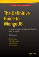
Let’s pretend I’m building a comments system like Disqus on MongoDB. (They actually use Postgres, but I’m asking you to use your imagination.) I plan to store millions of comments, but I’ll begin with four. Each has a timestamp and a quality rating, and one was posted by an anonymous coward:

{ timestamp: 1, anonymous: false, rating: 3 }
{ timestamp: 2, anonymous: false, rating: 5 }
{ timestamp: 3, anonymous:  true, rating: 1 }
{ timestamp: 4, anonymous: false, rating: 2 }

I want to query for non-anonymous comments with timestamps from 2 to 4, and order them by rating. We’ll build up the query in three stages and examine the best index for each using MongoDB’s explain().

Range Query

We’ll start with a simple range query for comments with timestamps from 2 to 4:

> db.comments.find( { timestamp: { $gte: 2, $lte: 4 } } )

There are three, obviously. explain() shows how Mongo found them:

> db.comments.find( { timestamp: { $gte: 2, $lte: 4 } } ).explain()
{
    "cursor" : "BasicCursor",
    "n" : 3,
    "nscannedObjects" : 4,
    "nscanned" : 4,
    "scanAndOrder" : false
    // ... snipped output ...
}

Here’s how to read a MongoDB query plan: First look at the cursor type. “BasicCursor” is a warning sign: it means MongoDB had to do a full collection scan. That won’t work once I have millions of comments, so I add an index on timestamp:

> db.comments.createIndex( { timestamp: 1 } )

The explain() output is now:

> db.comments.find( { timestamp: { $gte: 2, $lte: 4 } } ).explain()
{
    "cursor" : "BtreeCursor timestamp_1",
    "n" : 3,
    "nscannedObjects" : 3,
    "nscanned" : 3,
    "scanAndOrder" : false
}

Now the cursor type is “BtreeCursor” plus the name of the index I made. “nscanned” fell from 4 to 3, because Mongo used an index to go directly to the documents it needed, skipping the one whose timestamp is out of range.

For indexed queries, nscanned is the number of index keys in the range that Mongo scanned, and nscannedObjects is the number of documents it looked at to get to the final result. nscannedObjects includes at least all the documents returned, even if Mongo could tell just by looking at the index that the document was definitely a match. Thus, you can see that nscanned >= nscannedObjects >= n always. For simple queries you want the three numbers to be equal. It means you’ve created the ideal index and Mongo is using it.

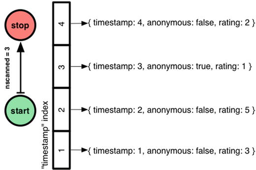
Equality Plus Range Query

When would nscanned be greater than n? It’s when Mongo had to examine some index keys pointing to documents that don’t match the query. For example, I’ll filter out anonymous comments:

> db.comments.find(
...     { timestamp: { $gte: 2, $lte: 4 }, anonymous: false }
... ).explain()
{
    "cursor" : "BtreeCursor timestamp_1",
    "n" : 2,
    "nscannedObjects" : 3,
    "nscanned" : 3,
    "scanAndOrder" : false
}

Although n has fallen to 2, nscanned and nscannedObjects are still 3. Mongo scanned the timestamp index from 2 to 4, which includes both the signed comments and the cowardly one, and it couldn’t filter out the latter until it had examined the document itself.

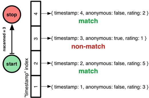
How do I get my ideal query plan back, where nscanned = nscannedObjects = n? I could try a compound index on timestamp and anonymous:

> db.comments.createIndex( { timestamp:1, anonymous:1 } )
> db.comments.find(
...     { timestamp: { $gte: 2, $lte: 4 }, anonymous: false }
... ).explain()
{
    "cursor" : "BtreeCursor timestamp_1_anonymous_1",
    "n" : 2,
    "nscannedObjects" : 2,
    "nscanned" : 3,
    "scanAndOrder" : false
}

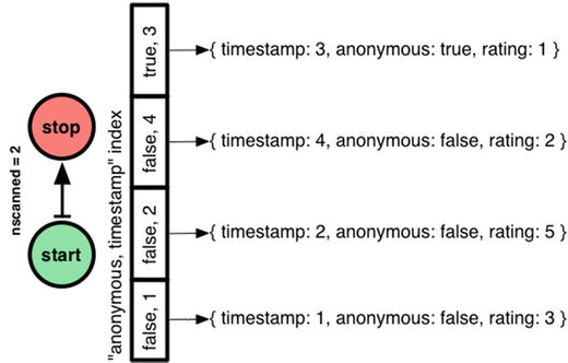
This is better: nscannedObjects has dropped from 3 to 2. But nscanned is still 3! Mongo had to scan the range of the index from (timestamp 2, anonymous false) to (timestamp 4, anonymous false), including the entry (timestamp 3, anonymous true). When it scanned that middle entry, Mongo saw it pointed to an anonymous comment and skipped it, without inspecting the document itself. Thus the incognito comment is charged against nscanned but not against nscannedObjects, and nscannedObjects is only 2.

Can I improve this plan? Can I get nscanned down to 2, also? You probably know this: the order I declared the fields in my compound index was wrong. It shouldn’t be “timestamp, anonymous” but “anonymous, timestamp”:

> db.comments.createIndex( { anonymous:1, timestamp:1 } )
> db.comments.find(
...     { timestamp: { $gte: 2, $lte: 4 }, anonymous: false }
... ).explain()
{
    "cursor" : "BtreeCursor anonymous_1_timestamp_1",
    "n" : 2,
    "nscannedObjects" : 2,
    "nscanned" : 2,
    "scanAndOrder" : false
}

Order matters in MongoDB compound indexes, as with any database. If I make an index with “anonymous” first, Mongo can jump straight to the section of the index with signed comments, then do a range-scan from timestamp 2 to 4.

So I’ve shown the first part of my heuristic: equality tests before range filters!

Let’s consider whether including “anonymous” in the index was worth it. In a system with millions of comments and millions of queries per day, reducing nscanned might seriously improve throughput. Plus, if the anonymous section of the index is rarely used, it can be paged out to disk and make room for hotter sections. On the other hand, a two-field index is larger than a one-field index and takes more RAM, so the win could be outweighed by the costs. Most likely, the compound index is a win if a significant proportion of comments are anonymous, otherwise not.

Digression: How MongoDB Chooses an Index

Let’s not skip an interesting question. In the previous example I first created an index on “timestamp”, then on “timestamp, anonymous”, and finally on “anonymous, timestamp”. MongoDB chose the final, superior index for my query. How?

MongoDB’s optimizer chooses an index for a query in two phases. First it looks for a prima facie “optimal index” for the query. Second, if no such index exists it runs an experiment to see which index actually performs best. The optimizer remembers its choice for all similar queries.

What does the optimizer consider an “optimal index” for a query? The optimal index must include all the query’s filtered fields and sort fields. Additionally, any range-filtered or sort fields in the query must come after equality fields. (If there are multiple optimal indexes for the current query criteria, MongoDB will use a previously successful plan until it performs poorly compared to a different plan.) In my example, the “anonymous, timestamp” index is clearly optimal, so MongoDB chooses it immediately.

This isn’t a terrifically exciting explanation, so I’ll describe how the second phase would work. When the optimizer needs to choose an index and none is obviously optimal, it gathers all the indexes relevant to the query and pits them against each other in a race to see who finishes, or finds 101 documents, first.

Here’s my query again:

db.comments.find({ timestamp: { $gte: 2, $lte: 4 }, anonymous: false })

All three indexes are relevant, so MongoDB lines them up in an arbitrary order and advances each index one entry in turn:

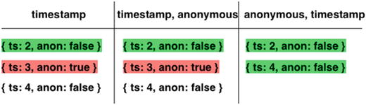
(I omitted the ratings for brevity; I’m just showing the documents’ timestamps and anonymosity.)

All the indexes return

{ timestamp: 2, anonymous: false, rating: 5 }

first. On the second pass through the indexes, the left and middle return

{ timestamp: 3, anonymous:  true, rating: 1 }

which isn’t a match, and our champion index on the right returns

{ timestamp: 4, anonymous: false, rating: 2 }

which is a match. Now the index on the right is finished before the others, so it’s declared the winner and used until the next race.

In short: if there are several useful indexes, MongoDB chooses the one that gives the lowest nscanned.

Equality, Range Query, and Sort

Now I have the perfect index to find signed comments with timestamps between 2 and 4. The last step is to sort them, top-rated first:

> db.comments.find(
...     { timestamp: { $gte: 2, $lte: 4 }, anonymous: false }
... ).sort( { rating: -1 } ).explain()
{
    "cursor" : "BtreeCursor anonymous_1_timestamp_1",
    "n" : 2,
    "nscannedObjects" : 2,
    "nscanned" : 2,
    "scanAndOrder" : true
}

This is the same access plan as before, and it’s still good: nscanned = nscannedObjects = n. But now “scanAndOrder” is true. This means MongoDB had to batch up all the results in memory, sort them, and then return them. Infelicities abound. First, it costs RAM and CPU on the server. Also, instead of streaming my results in batches, MongoDB just dumps them all onto the network at once, taxing the RAM on my app servers. And finally, MongoDB enforces a 32MB limit on data it will sort in memory. We’re only dealing with four comments now, but we’re designing a system to handle millions!

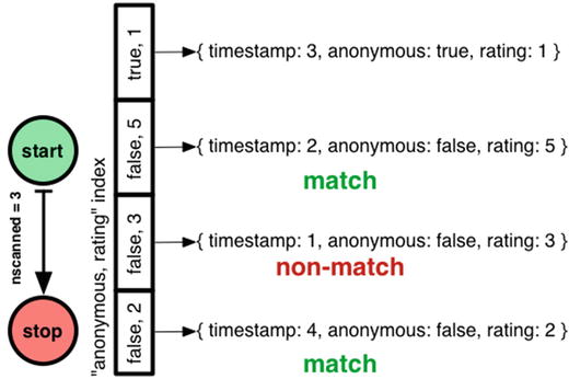
How can I avoid scanAndOrder? I want an index where MongoDB can jump to the non-anonymous section, and scan that section in order from top-rated to bottom-rated:

> db.comments.createIndex( { anonymous: 1, rating: 1 } )

Will MongoDB use this index? No, because it doesn’t win the race to the lowest nscanned. The optimizer does not consider whether the index helps with sorting.¹

I’ll use a hint to force MongoDB’s choice:

> db.comments.find(
...     { timestamp: { $gte: 2, $lte: 4 }, anonymous: false }
... ).sort( { rating: -1 }
... ).hint( { anonymous: 1, rating: 1 } ).explain()
{
    "cursor" : "BtreeCursor anonymous_1_rating_1 reverse",
    "n" : 2,
    "nscannedObjects" : 3,
    "nscanned" : 3,
    "scanAndOrder" : false
}

The argument to hint is the same as createIndex. Now nscanned has risen to 3 but scanAndOrder is false. MongoDB walks through the “anonymous, rating” index in reverse, getting comments in the correct order, and then checks each document to see if its timestamp is in range.

This is why the optimizer won’t choose this index, but prefers to go with the old “anonymous, timestamp” index which requires an in-memory sort but has a lower nscanned.

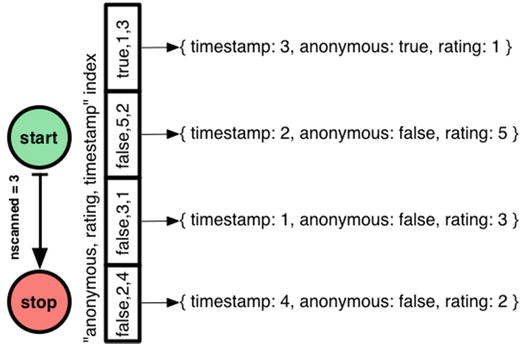
So I’ve solved the scanAndOrder problem, at the cost of a higher nscanned. I can’t reduce nscanned, but can I reduce nscannedObjects? I’ll put the timestamp in the index so MongoDB doesn’t have to get it from each document:

> db.comments.createIndex( { anonymous: 1, rating: 1, timestamp: 1 } )

Again, the optimizer won’t prefer this index so I have to force it:

> db.comments.find(
...     { timestamp: { $gte: 2, $lte: 4 }, anonymous: false }
... ).sort( { rating: -1 }
... ).hint( { anonymous: 1, rating: 1, timestamp: 1 } ).explain()
{
    "cursor" : "BtreeCursor anonymous_1_rating_1_timestamp_1 reverse",
    "n" : 2,
    "nscannedObjects" : 2,
    "nscanned" : 3,
    "scanAndOrder" : false,
}

This is as good as it gets. MongoDB follows a similar plan as before, moonwalking across the “anonymous, rating, timestamp” index so it finds comments in the right order. But now, nscannedObjects is only 2, because MongoDB can tell from the index entry alone that the comment with timestamp 1 isn’t a match.

If my range filter on timestamp is selective, adding timestamp to the index is worthwhile; if it’s not selective then the additional size of the index won’t be worth the price.

Final Method

So here’s my method for creating a compound index for a query combining equality tests, sort fields, and range filters:

1. Equality Tests—Add all equality-tested fields to the compound index, in any order
2. Sort Fields (ascending / descending only matters if there are multiple sort fields)—Add sort fields to the index in the same order and direction as your query’s sort
3. Range Filters—First, add the range filter for the field with the lowest cardinality (fewest distinct values in the collection), then the next lowest-cardinality range filter, and so on to the highest-cardinality

You can omit some equality-test fields or range-filter fields if they are not selective, to decrease the index size—a rule of thumb is, if the field doesn’t filter out at least 90% of the possible documents in your collection, it’s probably better to omit it from the index. Remember that if you have several indexes on a collection, you may need to hint Mongo to use the right index.

That’s it! For complex queries on several fields, there’s a heap of possible indexes to consider. If you use this method you’ll narrow your choices radically and go straight to a good index.

Specifying Index Options

You can specify several interesting options when creating an index, such as creating unique indexes or enabling background indexing; you’ll learn more about these options in the upcoming sections. You specify these options as additional parameters to the ensureIndex() function, as in the following example:

>db.posts.ensureIndex({author:1}, {option1:true, option2:true, ..... })

Creating an Index in the Background with {background:true}

When you instruct MongoDB to create an index by using the createIndex() function for the first time, the server must read all the data in the collection and create the specified index. By default, initial index builds are done in the foreground, and all operations on the collection’s database are blocked until the index operation completes.

MongoDB also includes a feature that allows this initial build of indexes to be performed in the background. Operations by other connections on that database are not blocked while that index is being built. No queries will use the index until it has been built, but the server will allow read and write operations to continue. Once the index operation has been completed, all queries that require the index will immediately start using it. It’s worth noting that when an index is built in the background, it will take longer to complete. Therefore, you may wish to look at other strategies for building your indexes.

Creating an Index with a Unique Key {unique:true}

When you specify the unique option, MongoDB creates an index in which all the keys must be different. This means that MongoDB will return an error if you try to insert a document in which the index key matches the key of an existing document. This is useful for a field where you want to ensure that no two people can have the same identity (that is, the same userid).

However, if you want to add a unique index to an existing collection that is already populated with data, you must make sure that you have deduped the key(s). In this case, your attempt to create the index will fail if any two keys are not unique.

The unique option works for simple and compound indexes, but not for multikey value indexes, where they wouldn’t make much sense.

If a document is inserted with a field missing that is specified as a unique key, then MongoDB will automatically insert the field, but will set its value to null. This means that you can only insert one document with a missing key field into such a collection; any additional null values would mean the key is not unique, as required.

Creating Sparse Indexes with {sparse:true}

Sometimes it can be worthwhile to create an index of only documents that contain an entry for a given field. For example, let’s say you want to index e-mails, and you know that not all e-mails will have a CC (carbon copy) or a BCC (blind carbon copy) field. If you create an index on CC or BCC, then all documents would be added with a null value, unless you specify a sparse index. This can be a space-saving mechanism as you only index on valid documents rather than all documents. Of course, this has an impact on any queries that are run and use the sparse index, as there may be documents that are not evaluated in the query.

Creating Partial Indexes

As of version 3.2, MongoDB can now create partial indexes. These are indexes that, like sparse indexes, only contain documents that match a given criteria. The criteria in these cases can take the form of a query specification for a document range. Let’s say you have a collection of foods that contains the name, SKU, and price of the foods. If you wanted to index the “expensive” foods by name, you would want to index only those foods that cost more than $10.00. To do this, you would can create an index as follows:

db.restaurants.createIndex(
   { name: 1 },
   { partialFilterExpression: { cost: { $gt: 10 } } } )

TTL Indexes

In computing terms, TTL (time to live) is a way of giving a particular piece of data or a request a lifespan by specifying a point at which it becomes invalid. This can be useful for data stored within your MongoDB instance, too, as often it is nice to have old data automatically deleted. In order to create a TTL index you must add the expireAfterSeconds flag and a seconds value to a single (noncompound) index. This will indicate that any document that has the indexed field greater than the given TTL value will be deleted when the TTL deletion task next executes. As the deletion task is run once every 60 seconds, there can be some delay before your old documents are removed.

Suppose for example that you want to automatically delete anything from the blog’s comments collection that has a created timestamp over a certain age. Take this example document from the comments collection:

>db.comments.find();
{
     "_id" : ObjectId("519859b32fee8059a95eeace"),
     "author" : "david",
     "body" : "foo",
     "ts" : ISODate("2013-05-19T04:48:51.540Z"),
     "tags" : [ ]
}

Let’s say you want to have any comment older than 28 days deleted. You work out that 28 days is 2,419,200 seconds long. Then you would create the index as follows:

>db.comments.createIndex({ts:1},{ expireAfterSeconds: 2419200})

When this document is more than 2,419,200 seconds older than the current system time, it will be deleted. You could test this by creating a document more than 2,419,200 seconds old using the following syntax:

date = new Date(new Date().getTime()-2419200000);
db.comments.insert({ "author" : test", "body" : "foo", "ts" : date, "tags" : [] });

Now simply wait a minute and the document should be deleted.

Text Search Indexes

MongoDB 2.4 introduced a new type of index—text indexes, which allow you to perform full text searches! Chapter 8 discussed the text index feature in detail, but it’s worth a quick summary here as we look at optimization. Text search has long been a desired feature in MongoDB, as it allows you to search for specific words or text within a large text block. The best example of how text search is relevant is a search feature on the body text of blog posts. This kind of search would allow you to look for words or phrases within one text field (like the body) or more (like body and comments) text fields of a document. So to create a text index, run the following command:

>db.posts.createIndex( { body: "text" } )

Now you can search using our text index with the text command. To do this, use the runCommand syntax to use the text command and provide it a value to search:

>db.posts.find({ "$text" : { $search: "MongoDB" } })

The results of your text search will be returned to you in order of relevance. You can make this search case-sensitive with the following:

>db.posts.find({ "$text" : { $search: "MongoDB", $caseSensitive : true } })

Dropping an Index

You can elect to drop all indexes or just one specific index from a collection. Use the following function to remove all indexes from a collection:

>db.posts.dropIndexes()

To remove a single index from a collection, you use syntax that mirrors the syntax used to create the index with ensureIndex():

>db.posts.dropIndex({"author.name":1, "author.email":1});

Reindexing a Collection

If you suspect that the indexes in a collection are damaged—for example, if you’re getting inconsistent results to your queries—then you can force a reindexing of the affected collection.

This will force MongoDB to drop and re-create all the indexes on the specified collection (see Chapter 9 for more information on how to detect and solve problems with your indexes), as in the following example:

> db.posts.reIndex()
{
     "nIndexesWas" : 2,
     "msg" : "indexes dropped for collection",
     "nIndexes" : 2,
     "indexes" : [
          {
               "key" : {
                    "_id" : 1
               },
               "ns" : "blog.posts",
               "name" : "_id_"
          },
          {
               "key" : {
                    "Tags" : 1
               },
               "ns" : "blog.posts",
               "name" : "Tags_1"
          }
     ],
     "ok" : 1
}

The output lists all the indexes the command has rebuilt, including the keys. Also, the nIndexWas: field shows how many indexes existed before running the command, while the nIndex: field gives the total number of indexes after the command has completed. If the two values are not the same, the implication is that there was a problem re-creating some of the indexes in the collection.

Using hint( ) to Force Using a Specific Index

The query optimizer in MongoDB selects the best index from the set of candidate indexes for a query. It uses the methods just outlined to try to match the best index or set of indexes to a given query. There may be cases, however, where the query optimizer does not make the correct choice, in which case it may be necessary to give the component a helping hand.

You can provide a hint to the query optimizer in such cases, nudging the component into making a different choice. For example, if you have used explain() to show which indexes are being used by your query, and you think you would like it to use a different index for a given query, then you can force the query optimizer to do so.

Let’s look at an example. Assume that you have an index on a subdocument called author with name and email fields inside it. Also assume that you have the following defined index:

>db.posts.createIndex({author.name:1, author.email:1})

You can use the following hint to force the query optimizer to use the defined index:

>db.posts.find({author:{name:’joe’, email: ’[email protected]’}}).hint({author.name:1, author.email:1})

If for some reason you want to force a query to use no indexes (such as wanting to prewarm your data), that is, if you want to use collection document scanning as the means of selecting records, you can use the following hint to do this:

>db.posts.find({author:{name: ’joe’, email: ’[email protected]’}}).hint({$natural:1})

Using Index Filters

As discussed earlier when we explained why you should use hint, there are occasions where you as the end user may have a better idea of which index to use for a given query. We looked at how to use the hint operator from the client side as a method of telling the system which index should be used. While this method is a good solution in many situations, there are some situations where modifying things from the client side may not be suitable, especially as each new index may mean a change to your hints. It is for this reason that the MongoDB team has introduced index filters. Index filters provide a temporary way for you to tell MongoDB that a particular “type” of query should use a particular index.

The first step in this process is to have a method to isolate a given type of query. This is done by finding a “Query Shape,” which consists of the query itself, any sort criteria, and any projection criteria. At this point, it’s best to leave abstraction and start working through this with a highly contrived and very simplified example of what a query shape would look like; so with that in mind, consider the following documents in a collection called “stuff”:

{ letter : "A", number : "1", food : "cheese", shape : "square" }
{ letter : "B", number : "2", food : "potato", shape : "square" }
{ letter : "C", number : "1", food : "ham", shape : "triangle" }
{ letter : "D", number : "2", food : "potato", shape : " triangle" }
{ letter : "E", number : "1", food : " ham", shape : "square" }
{ letter : "F", number : "2", food : "corn", shape : "circle" }
{ letter : "G", number : "1", food : "potato", shape : " circle" }

And assume that the following indexes exist:

{ letter : 1, shape : 1 }
{ letter : 1, number : 1 }

With this in mind, let’s say that you want to find all the letters greater than “B,” which contain “circle” sorted by their number using the following query:

> db.stuff.find({letter : {$gt : "B"}, shape : "circle"}).sort({number:1})

If you set the log level to 1, you can see the log output of this command with:

> db.adminCommand({setParameter:1, logLevel:1})

You can execute the query and get the output from the log file. This output shows the query execution stats so you can see what the chosen plan to run this query is:

2015-10-12T21:12:04.006+1100 I COMMAND  [conn1] command test.stuff command: find { find: "stuff", filter: { letter: { $gt: "B" }, shape: "circle" }, sort: { number: 1.0 } } planSummary: IXSCAN { letter: 1.0, number: 1.0 } keysExamined:7 docsExamined:7 hasSortStage:1 cursorExhausted:1 keyUpdates:0 writeConflicts:0 numYields:0 nreturned:2 reslen:275 locks:{ Global: { acquireCount: { r: 2 } }, Database: { acquireCount: { r: 1 } }, Collection: { acquireCount: { r: 1 } } } protocol:op_command 0ms

If you look at the output, you will see that the method for solving this query is an IndexScan (denoted by IXSCAN) of the {letter : 1, number : 1} index. Now, for the sake of understanding how to set an index filter, let’s say that hypothetically you want to enforce the use of the index {letter : 1, shape : 1} with our query.

Armed with these basic parts together, let’s assemble the command to set an index filter. The command in question is planCacheSetFilter and could be invoked as follows:

> db.runCommand(
   {
      planCacheSetFilter: "stuff",
      query: {letter : {$gt : "B"}, shape : "circle"},
      sort: {number:1},
      projection: { },
      indexes: [ { letter:1, shape:1} ]
   }
)
{ "ok" : 1 }

You can see that the projection is marked as an empty document. If you remember from earlier, a projection is the name in MongoDB for a query which returns only some part of document. If, for example, you wanted only to return the letter and shape, you would have a projection of {_id:0, letter:1, shape:1}. Remember, that the _id field is enabled in a projection by default. With the index filter set, run the query again and see the results:

> db.stuff.find({letter : {$gt : "B"}, shape : "circle"}).sort({number:1})

This results in the following output:

2015-10-12T21:19:02.894+1100 I COMMAND  [conn1] command test.stuff command: find { find: "stuff", filter: { letter: { $gt: "B" }, shape: "circle" }, sort: { number: 1.0 } } planSummary: IXSCAN { letter: 1.0, shape: 1.0 } keysExamined:7 docsExamined:2 hasSortStage:1 cursorExhausted:1 keyUpdates:0 writeConflicts:0 numYields:0 nreturned:2 reslen:275 locks:{ Global: { acquireCount: { r: 2 } }, Database: { acquireCount: { r: 1 } }, Collection: { acquireCount: { r: 1 } } } protocol:op_command 0ms

As you can see, you are now using the “desired” index. Another important thing to note is that the $gt in that query is significant, but the “B” value or “circle” value is not. If you run a query that looks for just {letter: "B", shape: "circle"}, it will default back to the {letter : 1, number : 1} index. However, if you were to query for {letter : {$gt : "C"}, shape : "square"}, then the index filter would kick in and function as desired.

Now that you have set an index filter, there are two other corollary functions of which you need to be aware. First is the planCacheListFilters function, which lists the current filters on a given collection. It is invoked and outputs as follows:

> db.runCommand( { planCacheListFilters:"stuff"})
{
        "filters" : [
                {
                        "query" : {
                                "letter" : {
                                        "$gt" : "B"
                                },
                                "shape" : "circle"
                        },
                        "sort" : {
                                "number" : 1
                        },
                        "projection" : {

                        },
                        "indexes" : [
                                {
                                        "letter" : 1,
                                        "shape" : 1
                                }
                        ]
                }
        ],
        "ok" : 1
}

The second is a function to remove any index filters, planCacheClearFilters. It is invoked almost identically to planCacheSetFilter:

> db.runCommand(
   {
      planCacheSetFilter : "stuff",
      query: {letter : {$gt : "B"}, shape : "circle"},
      sort: {number:1},
      projection: { },
      indexes: [ { letter:1, shape:1} ]
   }
)

This results in no longer having any filter set! As you have probably gathered, index filters are highly powerful in the right hands. They are also a little finicky to set up and need a bit of finesse to get going, a perfect tool for us as power users looking to optimize our MongoDB experience.

Optimizing the Storage of Small Objects

Indexes are the key to speeding up data queries. But another factor that can affect the performance of your application is the size of the data it accesses. Unlike database systems with fixed schemas, MongoDB stores all the schema data for each record inside the record itself. Thus, for large records with large data contents per field, the ratio of schema data to record data is low; however, for small records with small data values, this ratio can grow surprisingly large.

Consider a common problem in one of the application types that MongoDB is well suited for: logging. MongoDB’s extraordinary write rate makes streaming events as small documents into a collection very efficient. However, if you want to optimize further the speed at which you can perform this functionality, you can do a couple of things.

First, you can consider batching your inserts. MongoDB has a BulkWrite API that allows you to do large group inserts. You can use this to place several documents into a collection at the same time. This results in fewer round trips through the database interface API and thus higher throughput.

Second (and more importantly), you can reduce the size of your field names. If you have smaller field names, MongoDB can pack more event records into memory before it has to flush them out to disk. This makes the whole system more efficient.

For example, assume you have a collection that is used to log three fields: a time stamp, a counter, and a four-character string used to indicate the source of the data. The total storage size of your data is shown in Table 10-2.

If you use ts, n, and src for the field names, then the total size of the field names is 6 bytes, you can also use Object.bsonsize() from within the Mongo shell to get the size of an object. This is a relatively small value compared to the data size. But now assume you decided to name the fields WhenTheEventHappened, NumberOfEvents, and SourceOfEvents. In this case, the total size of the field names is 48 bytes, or three times the size of the data themselves. If you wrote 1TB of data into a collection, then you would be storing 750GB of field names, but only 250GB of actual data.

This does more than waste disk space. It also affects all other aspects of the system’s performance, including the index size, data transfer time, and (probably more importantly) the use of precious system RAM to cache the data files.

In logging applications you also need to avoid adding unnecessary indexes on your collections when writing records; as explained earlier, indexes take time and resources to maintain. Instead, you should add the index immediately before you start analyzing the data.

Finally, you should consider using a schema that splits the event stream into multiple collections. For example, you might write each day’s events into a separate collection. Smaller collections take less time to index and analyze.

Summary

In this chapter, we looked at some tools for tracking down slow performance in MongoDB queries, as well as potential solutions for speeding up the slow queries that surface as a result. We also looked at some of the ways to optimize data storage. For example, we looked at ways to ensure that we are making full use of the resources available to the MongoDB server. Finally, we reviewed MongoDB’s new storage engine WiredTiger and how you can use WiredTiger to drive further performance within your MongoDB instances.

The specific techniques described in this chapter enable you to optimize your data and tune the MongoDB system it is stored in. The best approach to take will vary from application to application, and it will depend on many factors, including the application type, data access patterns, read/write ratios, and so on.

¹Gory details: the scanAndOrder query plan “anonymous, timestamp” wins over the pre-ordered plan “anonymous, rating,” because it gets to the end of my small result set first. But if I had a larger result set, then the pre-ordered plan might win. First, because it returns data in the right order, so it crosses the finish line when it finds 101 documents, while a scanAndOrder query plan isn’t declared finished until it’s found all the results. Second, because a scanAndOrder plan quits the race if it reaches 32MB of data, leaving the pre-ordered plans to finish. I told you these details would be gory.