Chapter 4

Overview of the Most Important Renewable Energy Technologies

4.1 Basics About the Potential of Various Renewable Technologies

In the preceding chapters the finiteness of traditional exhaustible energy sources including their harm to the environment and mankind was discussed. If we just compare the reserves for the various exhaustible energies with the annual primary energy consumption, we can see in Figure 4.1 that with the exception of coal these reserves will only last for a few decades (see also [2-7]). However, if we compare this to the annual solar energy radiation we can easily see that even a substantial increase in exhaustible energies could never reach the input of the annual solar radiation. Taking a look at the various renewable technologies as seen in Figure 4.1 like wind, biomass, geothermal, wave and tidal as well as hydro energy, we realize when comparing their annual energy delivery to that of solar radiation on the continents that solar has by far the biggest contribution to offer [2-7]. It is therefore no surprise that solar will also have the most pronounced place within the portfolio of the future scenarios discussed in later chapters. Figure 4.1 shows the total annual renewable Energy input for each energy form. The technical potential given in Figure 4.1 for the various renewables has also been analyzed by WBGU [2-7]. The numbers they arrived at for the technical potential can be seen in Table 4.1. In addition this group also worked on a so-called “sustainable potential” which takes into account important restrictions. These are described in more detail in [2-7] by going from the “technical potential” to the “sustainable potential” and can be highlighted as follows for the individual renewable resources:

• Biomass should not compete with food production and biodiversity should be preserved
• Geothermal for electricity production is restricted to those regions which supply high temperature steam
• Hydro should take into account the methane emissions from flooded areas, the siltation of large reservoirs and the impact on biodiversity
• Wind is restricted by noise emissions near to buildings for on-shore farms
• Solar has limitations when solar farms are competing with food production

Table 4.1 Global potentials for renewable energy sources (for comparison: global primary (secondary) energy consumption in 2010 ~140 (90) PWh).

	Technical potential [PWh/year]	Sustainable potential [PWh/year]
Biomass	224	28.0
Geothermal	202	6.2
Hydro	45	3.4
Solar	78,400	2,800.0
Wind	476	280.0
total	79,347	3,117.6

Source: WBGU Flagship Report [2-7]

As a reminder, the split between the major renewable sources for the sustainable potential can be summarized as follows: 90% solar, 9% wind and 1% all other renewables (including hydro). We will later discuss a model where for the future secondary energy needs the fraction of solar is reduced to only 60%, that of wind increased to 20% and that of all other renewables substantially increased also to 20%.

It is often argued that land use for renewables may not allow to generate enough energy. Figure 4.2 demonstrates that this argument is wrong. If we used solar modules as of today we could produce the annual electricity of the world (~20,000 TWh) or the EU (~3,000TWh) as indicated by the two red areas. This already results from a simple calculation with conservative assumptions:

• 15% module efficiency (today even higher)
• With realistic solar insolation for the Sahara desert we have 1.8 kWh/W_{PV installed}
• Installation area = 2 x module area

The necessary area to cover the global electricity consumption can then be calculated as:

Similarly, the area needed to cover the annual European electricity consumption would be 150 × 150 km².

When I am showing such a relatively small area in lectures and discussions I mostly encounter disbelief – but check it out yourself! This little calculation should only demonstrate the small area coverage needed for the global electricity needs. The nice thing is that in many cases we can use areas already in use where there are buildings, parking lots and many other areas that could be covered with PV modules.

Similar examples could also be given for other renewable technologies.

4.2 Wind Energy

There are many excellent books and journals describing this renewable Energy form. A good overview is given by Darrell Dodge [4-1] and up-to-date market and technology information can be researched on the website of the European Wind Energy Association EWEA [4-2].

The history of wind power dates back more than 1,000 years ago. A vertical axis system was developed in Persia about 500–900 A.D. We know that similar vertical axis windmills were developed in China with one piece of documentation dating back to 1219 A.D. although it is believed that the windmill was invented in China as long ago as 2,000 years. The windmills were most commonly used for water pumping and grain grinding. The first illustrations of European windmills on the Mediterranean coast (1270 A.D.) show a four bladed mill with a horizontal axis. This type has a higher structural efficiency compared to the vertical axis due to less shielding of the rotor collection area. In the late 14^th century, the Dutch started to refine the tower mill design. An important improvement to the European mills was the introduction of sails. These could be formed to generate a higher aerodynamic lift and they provided increased rotor efficiency compared to the vertical axis mills. The next 500 years saw a continuous development and by the 19^th century the windmill sails had all the main features that we see today in the modern wind turbine blades. Famous windmills are the thousands of sail-wing windmills on the Lassithi plateau of Crete, which were built in the late 1800s and are indispensable for local farmers to pump water with many of them still in use today. The development of the multi steel-bladed water pumping windmill was perfected in the US during the 19^th century starting with four paddle-like wooden blades, followed by an increase in the number of thin wooden slats. Steel was used from 1870 onwards because it could be made lighter and worked into more efficient shapes. Between 1850 and 1970, over six million such small windmills were installed in the US alone.

The first large windmill to produce electricity was built as early as 1888 by Charles F. Brush in Cleveland, Ohio. The machine had a multiple-bladed rotor which was 17 meters in diameter and astonishingly operated 20 years long. The output was 12 kW which can be compared to the approximately 100 kW produced by today’s machines of the same diameter. Only a few years later, in 1891, the Dane Poul La Cour developed the first electrical output wind machine incorporating aerodynamic design principles. The use of 25 kW windmills had spread throughout Denmark by the end of World War I but came to an end due to cheaper and larger fossil-fuel steam plants. Also worth mentioning is the development of modern vertical axis rotors in France by G.J.M. Darrieus in the 1920s, further development of which had to wait until the concept had been reinvented in the late 1960s by two Canadian researchers.

A first utility-scale wind energy conversion system was developed in Russia in 1931 with the 100 kW Balaclava windmill. This system operated for about two years on the shore of the Caspian Sea, generating 200,000 kWh of electricity. The largest system was built in the US and was a 1.25 MW machine, installed in 1941(!) in Vermont. After only a few hundred hours of operation, one of the blades broke off, apparently as a result of metal fatigue. Obviously, the jump in scale was too big for the materials available. German engineers should have learned from this finding 40 years later, when they decided to build the 3 MW “GROWIAN” wind mill.

After the oil crisis in 1973, a government funded program was started in the US to test a variety of different small, medium and large wind turbine designs. Up to 3.2 MW horizontal axis and several vertical axis Darrieus machines were tested. In Canada there was even the installation of a 4 MW Darrieus machine within the Hydro-Quebec project Eole. This wind turbine operated from 1988 to 1993, generating about 12,000 MWh electricity [4-3]. Also in Germany a big technology program was initiated with substantial support from the government, the Great Wind Mill (GROWIAN = GROsse WIndenergie ANlage) with 3 MW power which was installed in 1983. Similar to the problems in Vermont (see above), the up-scaling was too dramatic and the windmill was decommissioned in 1987 after only a few hundred operational hours.

It is interesting to analyze why in the 1980s it was not possible to translate this technology driven program in the US into a commercial success with GWs of installed windmills. The major reasons for this were: too great an interference of political factors, too early a withdrawal of financial support and – most important in my point of view - technology push rather than market pull support. We will also be looking at more examples for other renewable technologies.

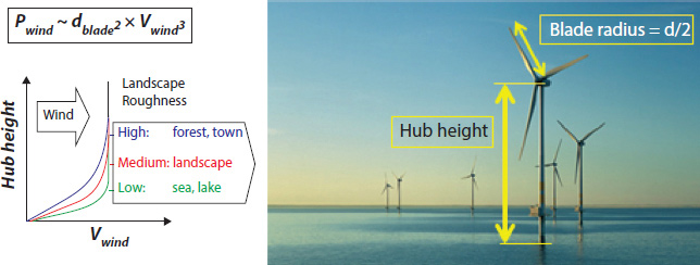
Let us now take a look at which factors will drive the further technology development in the future. In Figure 4.3 the windmill picture on the right shows a typical windmill with a tower and the electric generator at the top together with three blades, defining the radius of the rotor. It is important to understand that the power output of a given windmill is proportional to the third (!) power of the wind velocity. This means that an increase by only 20% (30, 50 or 100%) will increase the power output by a factor of 1.7 (2.2, 3.4 or 8). This is important for two reasons: one is that at a given site the wind velocity increases from ground to higher levels as seen in the left hand graphic of Figure 4.3 – very quickly at sea or on large lakes and much less in forests or towns, where the landscape roughness at lower levels degrades the wind velocity. This is the reason why windmills get higher and higher with their hub height. The other reason is that the annual output of a windmill at a given site varies quite significantly from year to year as the average wind velocity changes. Another important factor which determines the power output is the radius of the blade (or diameter of the spinning rotor). This dependence is proportional to the square of the blade size.

The continuous development over the last 20 years driven by market pull programs like the feed-in tariff developed in Germany (and explained in more detail in the next chapter) is illustrated in Figure 4.4.

As can be seen nicely, the factor of up-scaling in terms of power output or rotor diameter is only ever in the range of two to three and not – like in the case of the GROWIAN an up-scaling factor of 100 (30 kW to 3 MW). Unsurprisingly we now have 5 MW windmills in operation and the further development towards 10 and even 15 MW per machine is underway by further increase of hub height and rotor diameter. Another impressive increase due to the above mentioned dependencies is the power output at a given site for a single windmill increasing from 35 MWh to 1,250 MWh and 17,000 MWh for the 30 kW, the 600 kW and the 5 MW machine, respectively. For each doubling of installed power capacity there is an increase by almost a factor of 3 in energy output.

For a new industry, it is important not only to develop the respective product – in our case the windmill – but additionally the infrastructure and auxiliary systems also need to become large scale. In the case of windmills, this can be impressively seen by looking at Figure 4.5, which shows the installation of a 5 MW machine. The large cranes are now available in sizes and quantities which make it possible to install many big windmills in a short period of time.

The next big challenge is the development for off-shore windmills. One of the driving factors is the high wind velocity as previously explained. But even more important is the fact that unlike on-shore, where the wind only blows 1,500 full load hours, this increases greatly with off-shore to 3,000 up to 4,000 full load hours. This becomes important in view of the future of our 100% renewable goal. But before this can be utilized we have to overcome some technical hurdles. Firstly, the harsh environment – waves, strong wind and corrosion due to salt – and again the infrastructure to transport the big components and install them with specially constructed ships.

But not only the building of GW off-shore wind parks is an important piece of additional work that needs to be done. All the TWh of electricity that are produced at an off-shore park then have to be transported to the millions of electricity users, which means electricity transportation firstly to land and then distribution via High Voltage grids to the metropolises for usage.

While the generation cost for large on-shore windmills today are in the range of 5 €ct/kWh, the cost is much higher for off-shore production. It is not known today what the real lifetime for off-shore windmills will be in the future, especially taking into account the harsh environment. In order to account for this uncertainty, the feed-in tariff paid in Germany for such projects is in the range of about 18 €ct/kWh – well above even small roof-top PV systems. This does not include the connection from the off-shore plant to the coast, which adds another one to two Euro cents per kWh.

How did I calculate this connection cost number? I listened a lecture by Prof. Breitner from the University of Hannover, in which he reported on three specific investment numbers for currently installed wind-parks in the North and Baltic Sea: for a 580 MW (85 km subsea cable), 1,200 MW (125 km subsea cable) and a 800 MW (75 km subsea cable) off-shore wind-park the investment by the company Tennet was €700 million, €1,200 million and €850 million, respectively. If we simplify this to make it easy to remember, we can say that in all three cases the connection cost was about €1 billion per GW or €1/W_{wind power installed}. Knowing that in Germany a PV system in 2011 had a generation cost of about 20 €ct/kWh at a 2.5 €/W installed system price, 20 years of depreciation and 1,000 full load hours, we can easily calculate the following:

The result depends on whether we assume the same depreciation of 20 years or a 40 year depreciation for the electricity grid.

In Table 4.2, the cumulative installed wind power at the end of 2012 for the Top 10 countries together with their respective share as well as the ranking for the installations in the year 2012 are summarized [4-4].

Table 4.2 Cumulative (2012) and annual wind power installations for the Top 10 countries in 2012 and 2006 for comparison.

When comparing the annual installations in 2006 and 2012, we see that the global installations went up by a factor of 3 (which corresponds to an annual growth rate of 20%). It is impressive to see how particularly China has increased its wind power installations. China went from No. 5 to No. 1 in only 6 years by increasing the installations by a factor of 10(!). In the US, the factor of increase is merely 5, Great Britain and Italy increased their installations by a factor of 3, India, Germany and Canada increased theirs only slightly by a factor 1 to 1.5 while in Spain a decrease of 20% can be observed. This overview of annual installations in the different countries is even better reflected in the cumulative installations. From 2006 until 2012, China went up from only 2.6GW to 75GW (almost a factor of 30), the US figures increased from 6.3GW to 60GW (a factor of ~10), France’s numbers went from 1.6GW to 7.6GW (a factor of 5), cumulative installations in Italy and the UK only quadrupled, in Portugal and India it tripled, Spain doubled their cumulative installations, while Germany only increased them by a factor of 1.5. Denmark, which was not among the top 10 in 2006 and 2012 in terms of annual installations, is remarkable in that at the end of 2011 the cumulative installations in this rather small country contributed almost 26% to the annual electricity consumption in Denmark. This is the highest share of wind power penetration in one single country. Even if we add the installations in all EU countries together in 2012, we obtain about 8 GW [4-5]. This places the EU before the US but is still only 1/2 of the Chinese market. Only a few years ago, it was mainly European companies together with GE Wind Energy from the US that exported windmills to these countries. This has drastically changed in only a few years. The increased installations, especially in China, have been utilized for the creation of companies producing windmills including all necessary components (blades, transformers etc.) as seen in Table 4.3 [4-6,7].

Table 4.3 Top 10 manufacturers in 2010 and 2012 together with comparison in 2005.

Comparing the 2010 and 2005 data, only the market leader Vestas could maintain the pole position, although this was accompanied by bisecting its market share. Similarly, the big ones in 2005 from the US and Europe also bisected their market share (GE Wind energy, Enercon and Gamesa), only Siemens Wind Power and the Indish Suzlon Group could maintain their (small) market share. The Chinese manufacturers took advantage of their strongly increased home market by impressively increasing their capacities: Sinovel, the new No. 2, overtook GE Wind Power (which became No. 3) by increasing their capacity by a factor 15. Goldwind even increased their capacity 25 fold, making them No. 4. Dongfang and United Power from China were not visible in 2005 but could gain market positions 6 and 10, respectively. Other Chinese companies like Mingyang, Sewind and Hara XEMC, listed as No. 11, 14 and 15 in the world, respectively, are emerging to increasingly challenge the positions of the traditional market leaders from Europe and the US. In summary, in just five years the Chinese manufacturers increased their global market share from about only 3% in 2005 to an impressive 35% in 2010. The picture in 2012 changed due to a decrease in the Chinese market share within the Top 10 to 26%. This change was mainly caused by a market share doubling of the European company Siemens Wind Power and a significant drop in market share of the Chinese companies Sinovel and Goldwind.

The ever increasing appetite for energy in China paired with huge amounts of money to boost investments for capacity increase makes this country unique in the world. Many studies conclude that China will become the biggest economy after 2030. However, if the growth of the Chinese industry continues at a similar pace in the coming years with European and US growth being significantly lower and renewables being a fast growing sector worldwide, it will not take another 20 years and China could well overtake the US as the biggest worldwide economy much sooner. Especially the growth of installed systems has a very positive effect: as will be shown in a later chapter the increased global cumulative volume – to which China makes a large contribution – will be a solid basis to further drive down the price for wind energy machines thereby making wind power economically favorable to conventional fossil and nuclear power generating systems.

4.3 Solar Thermal Collectors and Concentrators

4.3.1 Historical Development

The power of concentrated sunlight is already described in an ancient Greek tale, where the famous Archimedes is said to have defeated the Roman fleet in 213 BC by using glasses to concentrate solar rays and to set the Roman ships on fire. However, this did not help him and a year later he was killed by a Roman soldier before Syracuse was conquered by the Romans.

In 1767 the Swiss scientist Horace de Saussure developed the first cone shaped solar collector for cooking purposes. This was a glass covered “hot box” design which made use of the discovery that sunlight passes through glass, gets absorbed at surfaces painted black inside the box and the resulting heat cannot escape through the glass, thereby warming up the box to more than 100°C. This is more or less the principle of solar thermal collectors today.

In 1816 Robert Stirling developed a hot air engine, the principle of which is still elaborated today in the Stirling cycle engine. The air contained in a cylinder makes four cycles utilizing the energy provided by an external heat source: heating, expansion, cooling and compression to produce rotational motion. There may be a revival of this technology in the coming years together with solar dish systems which I will describe later.

Almost 100 years after the hot box experiments, Augustin Bernard Mouchot continued with this development and in 1872 he presented a solar powered steam engine using a truncated cone reflector (inverted lamp shade) with ½ horse power (hp). A few years later, in 1878 he used a 4m diameter mirror and 80l boiler to make ice using solar power, which was quite a sensation in those days in France during the Paris exhibition. Other developments during this time occurred in Egypt where John Ericsson developed a parabolic trough in 1883 for pumping water, which was very similar to today’s Solar Thermal Concentrators. In 1878 in Bombay, William Adams built a central receiver which contained most of the features of modern prototypes in this technology.

Unfortunately, these efforts did not lead to commercialization although the underlying ideas of why more solar should be used were quite similar to today’s considerations. In the Victorian 18^th century some concerns were raised about the availability of coal to power the energy needs for the industrial revolution which were very similar to today’s fears about peak oil and gas. The fundamental reason why solar thermal did not make it in the past but will be able to take over today is that in the early 20^th century, oil became a much easier to handle secondary energy form especially to satisfy the needs that would arise in the upcoming First World War. Today, we can build on a portfolio of already proven renewable technologies with very competitive prices with the prospect of further price decrease compared to the increasing prices for conventional energy sources. A nice overview of this historic development is given by Magdi Ragheb [4-8].

The use of solar thermal today is split into two fundamentally different applications: firstly, domestic hot water and heat generation through flat plate collectors or vacuum tube collectors and secondly, solar thermal concentrating systems for electricity generation. The first category uses heated water at temperatures in the range 80 – 120°C for domestic use and 120 – 300°C for process heat for industry, while the second one heats special fluids to temperatures of 300°C to 600°C and a connected heat exchanger produces steam for electricity generation. Both categories can be combined with heat storage systems ranging from daily cycles up to seasonal storage of heat.

4.3.2 Solar Thermal Collectors

Two different designs for solar thermal collectors have evolved today: flat plate and tube collectors. The first category uses about 2m² of specially coated metal sheets as an absorber. The coating should have a high absorbance for the solar spectrum and at the same time a low emissivity in the infra-red (heat radiation). The coating can be applied via vacuum deposition processes (e.g. sputtering) or via electro-chemical coating. Until recently the metal sheets were made of copper. To transfer the heat from the coated metal sheet, a metal coil is welded to the absorber where a fluid circulates which consists of water plus e.g. glycol to prevent freezing of the heat exchange medium at low temperatures – especially at times without sunshine. The absorber is normally placed in a box covered by a glass sheet.

The second category uses glass tubes (typically 2m long with a diameter of 50–100mm), where absorption again occurs via a coated metal stripe situated in the glass tube or through a second coated glass tube with a smaller diameter through which the heat exchange medium is circulated. For better insulation, the volume between the outer and inner glass tube is evacuated (“vacuum solar thermal collectors”). Several glass tubes are mounted in a box and interconnected.

The system topography is also divided into two different categories: thermosyphon and external storage tank systems. The first system has the storage tank integrated and mounted just above the box containing the absorber. This simple approach utilizes the fact that hot water climbs up into the tank and then flows down through gravity when needed in the household. The disadvantage is the ugly look as there is no chance to integrate these tanks nicely and homogeneously into or onto roofs. If used on flat roofs which are common in many southern countries this concern is of less importance. The second system, where the tank is normally situated in the basement of houses must integrate an electrically operated pump which circulates the heat exchange medium.

Warm water for a household: Typical parameters for the supply of hot water during spring, summer and autumn in a typical single or multi-family house are as follows: collector area about 6m² and a 3001 storage tank. Prices in 2012 were about €4,000 for flat plate and €7,000 for tube collectors. A typical cost split is 50% for the collectors, 25% for the storage tank and 25% for the pumping system and installation. It is important to note that the efficiency for a traditional oil or gas fired hot water supply is typically at its lowest in summer times where (almost) all warm water can be supplied by the solar system.

Solar thermal collectors for warm water and heating support: In cases where a household would also like to use the solar water heating as a heating support especially in spring and autumn but also partially in winter, the system must be bigger in size. Typically 15m² collector area together with an 8001 storage tank should be installed. Prices are in the range of about €10,000 for a flat plate system. In order to make best use of the solar heated water for heating purposes it is desirable to have under-floor heating instead of radiators.

Technology: the major cost component for the flat plate collector is the absorber with ~50%. This used to be copper (Cu) in the past, but with the substantial Cu metal price increase (€3/kg to €7/kg from 2005 to 2011 at the London Metal Stock exchange, LME) the coated 0.2mm Cu sheet will be replaced by a coated 0.5mm Aluminium (Al) sheet, which should result in a 35% cost reduction for the absorber. The next step will be the replacement of the Cu piping with Al pipes. In the latter case, appropriate corrosion protection must be implemented. It is important to note that R&D is important for further cost decrease despite the general belief that flat plate collectors are low-tech products.

Thermal power instead of collector area: in public debates the measuring of solar thermal systems in m² collector area does not reflect the “real power” of such devices. Therefore an attempt was made by the IEA [4-9] to convert the collector area into the corresponding power at peak sunshine. The proportionality factor was determined at 0.7 kW_th for every m² of collector area. For the conversion of thermal power into the energy produced within a year as a mean average, the bank Sarasin assumed an energy output of 700 kWh for 1kW_th (more in the South, less in the North, proportional to the average global solar irradiation). A more general conversion function for various collector types and irradiation levels is given in [4-10].

The future of solar heating: While it is important to highlight the immense energy saving potential in today’s times where almost half of the secondary energy of countries is used for heating purposes, one must remember that in future there will be an interesting competition between alternatives in serving a specific energy need cost effectively and energy efficiency measures. In the case of solar thermal needs, even today in most houses, we have the situation that due to insufficient wall and window insulation most of the annual secondary energy is used for heating. As long as this situation continues, it makes a lot of economic and environmental sense to invest in solar thermal systems. For new future houses (well insulated with less than a tenth of the heating requirements of the old generation, it may be useful to consider a different approach from a total cost of ownership point of view. For instance, the complete piping and central heating boiler assisted by the thermal collector system could be avoided by providing the small amount of residual heat through electrical heating – but only if this electricity originates from renewables, including the electricity for heat pumps. As today’s investments in solar thermal systems will pay off in less than 10 years and since the replacement of existing houses with new ones is not likely to occur soon, one should encourage every home owner to invest in solar thermal systems for the time being. However, when looking at the longer time frame towards 2030 or even 2050, the dramatic decrease in required energy for heating and cooling due to proper insulation and the possibility of having water heated by electricity (resistance heating or via heat pump) should be taken into account and a simple extrapolation of today’s thermal energy needs to the future may result in fundamental errors and the total of installed areas for thermal collectors would be much too high.

Regional installations: it is interesting to see how the use of solar thermal systems developed in different regions in the world in the past and where the biggest momentum can be observed. As summarized in Table 4.4 it is again China which has installed most systems in the past with almost 200 million m² (corresponding to 136 GW_th). Almost ten times fewer installations were realized in the EU27 and Turkey, which both have a similar volume. The next group of 7 regions has an additional factor of between 3 and 10 times less, although there could be many more installations based on population and heat requirements: the US should have at least the same as the EU27 and India and Australia could also have a much higher installation base. Similarly, the annual installations in 2010 show China as the clear front runner with almost 50 million m² (34 GW_th), followed by the EU27 with 3.1 million and Turkey with 1.7 million m², with the other regions showing much less. When using an average of 700 kWh/kW_th there was a remarkable heat production of 133 TWh in 2010 with an annual addition of 28 TWh.

Table 4.4 Cumulative and annual solar thermal installations for the TOP 10 countries worldwide in 2010 [4-11].

Unlike in the wind sector, in the PV and solar thermal concentrator industry there are not just a few big, mostly market-listed production companies but a huge number of small and medium enterprises, most of them – unsurprisingly – in China, but also in Europe. It is interesting to remember that the glass tube absorber technology which dominates the Chinese market was originally a development by Dornier in Germany many years ago. As there was no interest in this technology in Europe in those days, they licensed their technology to China.

4.3.3 Solar Thermal Concentrating Systems for Electricity Production

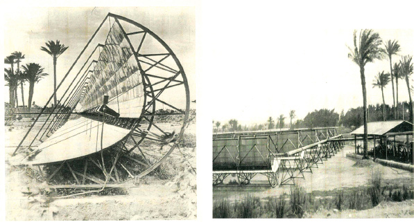
The first Concentrated Solar Power (CSP) plant, very similar in design to today’s systems was the “Solar Engine One”. It was originally developed by the USA inventor Frank Shuman by using a series of hot boxes which were replaced by parabolic mirror concentrators as suggested by Charles Vernon Boys. The system was built in 1912 in Al Maedi near Cairo, Egypt, and started operation in 1913. It is shown in Figure 4.6. It consisted of five parabolic concentrating reflectors, each 62m in length and 4m in width, oriented in a north-south direction together with a mechanical tracker system which kept the mirrors facing towards the sun throughout the day. The steam engine was shipped from the USA and had an equivalent of 55 hp, enough to pump ~27,000 liters of water per minute from the river Nile onto desert land. It was the First World War in 1914 which abruptly put an end to this technological success story: all system engineers left Al Maedi and a British army contingent dismantled the system to use the raw materials for war efforts.

The tremendous development of the internal combustion machine in the first half of the 20^th century, based on burning oil, was driven by the needs of all transportation purposes – cars, trucks and buses, ships and planes. The increased findings of oil fields in these times led people to believe that besides oil for transportation and coal for electricity production nothing else was needed for energy supply. The introduction of nuclear power after World War II (“Atoms for Peace”) empowered the belief that fossil and nuclear could power the world for the foreseeable future. It is no surprise that the renewable technologies, like Solar Thermal Electricity, were forgotten.

It was notably the first oil price shock in 1973 that people realized that oil – and also the other exhaustible primary energy sources – were finite and, additionally, may cause problems to our climate by warming the atmosphere due to CO₂. This initiated a huge R&D effort, especially in the USA where national laboratories, like SANDIA, were given large amounts of money to look for “alternatives” – which was the preferred name for “renewables” in these days. A major effort was undertaken in the field of Photovoltaics, wind power and also Solar Thermal Concentrators. Europe also developed different forms of Solar Thermal Concentrating Systems. The block diagram for Solar Thermal Concentrators is shown in Figure 4.7 and basically consists of the Concentrating Solar Thermal Field and a more conventional power block.

As an option, one could add a conventional gas or oil heated steam production and/or a thermal energy storage to prolong the time of electricity production after sunset.

The different technologies for the Concentrating Solar Thermal Field can be seen in Figure 4.8 which shows the state of the art parabolic trough as well as dish and solar tower systems.

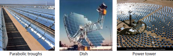
Technology: The most matured solar thermal power technology is the parabolic trough system. The rough cost split for such systems is 45% for the solar field, 20% for the power block and Heat Transfer Fluid, 25% for the Balance of Plant and others, 10% for services and site work. Obviously there is room for technological improvement for the solar field in both directions, which could reduce the cost of the running meter of the absorber and concentrating network as well as the cost per power unit by working at higher temperatures because of increasing efficiency in the power block. For the remaining 55% of the cost, there can unfortunately only be a cost decrease through increasing efficiency due to matured technology in the components used (turbine and associated components for producing electricity).

For the solar field there are two major components which can be optimized: the concentrating mirror and the receiver, which determines the efficiency of the system together with the heat transfer fluid.

Today the mirrors consist of 4-5 mm glass with sputtered silver to form the mirrors. These have a weight of ~ 10 kg/m². In the future, UV stabilized mirror film (ReflecTech^TM) laminated on aluminium may be used with a much lower weight of ~ 3.5 kg/m², thereby minimizing the structure cost. An additional cost decrease could come about through the use of small stripes of Fresnel lenses below the receiver which would further decrease the structure and tracking cost.

The heart of a STC system is the receiver. The state of the art today is produced by the company SCHOTT. With their PTR^TM70 receiver the following characteristics are obtained: solar selective coating on stainless steel (diameter 70mm) with high solar absorbance (>95%) and low thermal emittance (<10% at 400°C), surrounded by vacuum sealed glass (diameter 125mm) with glass transmittance > 96%, aperture length >96%. The bond between the glass and the steel tube at the interconnections between receiver tubes is important, as this may cause cracks due to temperature change from minus degrees Celsius at night to ~400°C at working conditions. SCHOTT was able to match the expansion coefficient of these two materials within the needed temperature range, thereby decreasing this defect. The great achievements of the receiver technology also present the problem of this technology: when looking at the technical numbers it can be concluded that the scope for a further increase in performance is only limited. There is no major technology development foreseen that would substantially decrease the specific system cost – mainly economy of scale and some material optimization can further decrease the cost per meter, including the interconnection.

Another limitation to the reduction of the specific system cost is the power block which is well developed – not only for this application. Hence the specific price ($/W) for this item will not decrease when increasing the volume of STC installations, but will develop in line with the world price for turbines in general.

After a quick decrease of the LCOE (levelized cost of electricity) in times when SEGS (Solar Electricity Generating System) I to IX were installed in the USA which added cumulative volume, further development has reached a point of saturation for reasons described above and lies today in the range of €ct18/kWh. This is about two to three times as high as for PV systems installed in similar locations. For the large green-field – or better yellow desert – PV systems, an important competitor to CSP, besides flat-plate PV, is the concentrated PV (CPV) system, which is well suited in large centralized systems in areas with high direct sunlight. Another advantage of PV systems is the absence of water needs which, however, is necessary for the cooling towers for CSP systems. Dry cooling towers can also be used with the disadvantage of substantially lower efficiency leading to a higher cost.

Another added value of STC systems is the storage of heat in phase change materials like molten salt to continue producing electricity after sunset. This enables a continuous production of electricity with stored heat from the sunshine hours during the night. The cost for storing heat per kWh electricity produced afterwards is substantially lower than the storage of electricity in electrochemical batteries. Depending on the price development for future batteries, this advantage may be an important added value for STC’s with integrated heat storage.

A major decrease in specific cost could be envisaged if one could substantially increase the temperature of the Heat Transfer Fluid (HTF). Today’s heat transfer oil limits this temperature to about 400°C thereby limiting the Carnot efficiency of the system (see also Table 4.8). If this could be replaced, either with water as a HTF for the production of steam directly, or with a still to be developed oil alternative, this temperature could be increased to 500°C or maybe 600°C thereby increasing the Carnot efficiency of the power block. This level of efficiency increase – if all other specific cost components could be kept at the same level – would then proportionally decrease the LCOE of STC produced kWh. This is the main reason why I personally still see a great future for this technology but only if this temperature increase of the HTF can be achieved. It will be interesting to see the performance of a recently started parabolic trough system (“Archimede” in Sicily) where water is no longer used to be heated in the receiver but instead a special molten salt is used. This enables an increase in the inlet temperature to above 500°C, thereby increasing the efficiency of the system. In addition, the same hot molten salt may also be used to store the heat in tanks for later electricity production at times when the sun is no longer shining. If these projects are not able to demonstrate this increase of efficiency it could well be that the parabolic trough technology may come to an end. This could then be the driving force to push the solar tower and dish technology as there will be higher temperatures anyway and this offers the potential to increase efficiency and in parallel to decrease the cost.

4.4 Bioenergy: Biomass and Fuel

An excellent overview of this subject can be found in WBGU [4-12]. Until recently (2005) bioenergy contributed ~60% to the 13% renewables share of primary energy. The breakdown of the ~14 PWh bioenergy is summarized in Table 4.5.

Table 4.5 Categories for bioenergy (~2005).

Category	% of total bioenergy	Energy [TWh]
Traditional (firewood for cooking & heating)	86.0	11,954
Modern bioheat	7.5	1,043
Biopower (corresponding to 45 GW)	4.3	598
Biofuel
# bioethanol	1.8	250
# biodiesel	0.4	56
Total	100.0	13,900

Although most discussions in our Western hemisphere are centered around the topic of biofuel, it is often forgotten that this is only a very small part (2.2%) and that the vast majority of bioenergy (86%) is used in form of wood for cooking and heating in developing countries. These ~12 PWh mainly from firewood could be replaced much more comfortably and environmentally friendly with new renewable sources like PV, wind and solar thermal. Biofuel only makes up a share of 16% of the rest of 1.9 PWh.

• For biopower there are many discussions on the topic of how to split the land use between agriculture for food production and plants for energy production (electricity, heat and transportation). There are many detailed studies which try to demonstrate that there is sufficient arable area for agriculture and also enough room for the production of biofuel and biomass for electricity production [4-13]. There are also many discussions derived from the problems with 1^st generation biofuels and the introduction of a 2^nd generation. This would use non-food lingo-cellulosic feed stock. While the 2^nd generation of bioenergy does make sense this is not the case for the 1^st generation as demonstrated below in a comparison between biomass production and state of the art renewable technology (PV and/or wind) on the same area of land: For electricity production from biomass we have numbers available [4-12] on how many MWh of electricity can be produced annually using the most advanced crops and technologies. These numbers are in the range of ~14, 17, 50 and up to 64 MWh per hectare for wheat, corn, sugar cane and best energy grass, respectively. Very often it is forgotten that the energy content per hectare (ha) is normally given as fuel energy. If we want to compare these numbers with electricity production from renewables, they must be divided by at least a factor of 2. In contrast we may compare this with the electricity production per hectare with today’s PV technologies. If we conservatively assume a mere 10% of module efficiency, the modest solar irradiation in Germany with 1,000 kWh/kW_installed and an area coverage of 50%, we obtain 1,000 kWh/kW_installed x 1 kW_installed/10 m² x 10⁴ m²/ha x 0.5 = 500 MWh/ha which is more than 10 times the electricity produced from the best and fastest growing plants – and we did not even consider the water and fertilizer that would be needed for the biomass production. This factor 10 doubles if we calculate the production for sunny regions with twice as much sunshine as Germany, and doubles again to 40 if we install modules with 20% efficiency, which is already available today. Additionally, there is the possibility of a “double harvest” [4-14]: If one were to mount the modules high enough for a small tractor to pass below, one could even plant vegetables for local use below those modules (in regions like Germany, not in the desert, which would not have allowed crops to grow anyway).
• For biofuel a comparison between electric cars and combustion machines fueled by biofuel shows without any doubt that the (renewable) electricity pathway is by far superior. With the fastest growing plants we have 64 MWh/hectare or 64 kWh/(10 m²). Assuming 5 1/(100 km) (the energy content of 5 liter of petrol corresponds to 45 kWh) we can drive a traditional car for 140 km per year based on an area of 10 m². In contrast we have conservatively for a 10 m² roof mounted PV in Germany ~1,000 kWh (only 10% efficiency). With ~15 kWh/(100 km) for a 4 passenger electric car we can drive ~6,700 km with the same 10 m² – which is more than 100 times the distance with biofuel under optimal conditions! Using 20% modules the distance increases to 13,400 km which covers almost the annual needs for an average commuting car. In sunny regions with twice the output compared to Germany, the above numbers double again towards ~27,000 km/year which is more than 400 times the distance which can be covered with biofuel.

In summary, it can be stated that 1^st generation bioenergy would be the wrong way to go for future energy supplies, both for electricity production and transportation.

4.5 Photovoltaics

This technology will be described in detail in the next two Chapters 5 and 6. In the context of the various renewable technologies it is, however, important to emphasize some of the specific aspects of this fascinating technology. While at the end of the 1990s it was widely believed that this way of producing electricity is the most elegant one, there was also a general understanding that this technology, which was at the time the most expensive one, would still need some decades and technological breakthroughs in order to become competitive. Due to forward-looking market support programs notably Feed-in tariff programs in Switzerland and Germany this technology could benefit from the well-known learning effect which is well recognized in other industries (Price Experience Curves for mass produced high-tech products, to be discussed in chapter 7). In essence, there is a close relationship between the price and the cumulated volume of such mass produced goods and for a given product there is a specific price decrease with every doubling of this cumulated volume. In the case of PV modules and inverters there is a 20% price decrease – also expressed as Price Experience Factor (PEF) 0.8 – with a doubling of cumulative volume. Due to the above mentioned support programs the market growth in the first decade of this century was an unforeseeable 50+% per year which boosted cumulative volume from 1.4GW in 2000 to an unanticipated 40 GW in 2010 and 100 GW by 2012! This implies a doubling of the cumulative volume by 2010 (6 times by 2012) which with the above mentioned PEF results in an expected price decrease of (0.8)⁵ = 0.33, meaning that the price in 2010 is 1/3 of what it was in 2000 (~1/4 in 2012). While in 2010 the actual module prices were slightly above the expected number, we have seen an additional decrease in 2012. This is due to a very high production capacity increase, notably in China, resulting in severe overcapacity.

On the one hand this situation is very problematic for the manufacturers and there is a widespread belief that only a fraction of the biggest and strongest will survive. On the other hand, this gives system integrators the chance to compete against traditional electricity generating technologies in new applications and countries without support programs. An example is the addition of PV systems to an existing diesel gen(eration) set, thereby saving fuel resulting in overall cost reduction for the user (“fuel saver mode”). This will again boost the market growth and with new technologies for module production, as discussed in chapter 8, the production cost will allow for positive margins at today’s prices.

In 1999 I sketched the PV generation cost as a function of time as shown in Figure 4.9. I restricted myself to the growth which was experienced in the decade 1990 to 2000, which was ~15% per annum. With this annual growth the cumulated volume would only have increased twofold, resulting in a price of only 2/3 in 2010 compared to 2000 (~40 €ct/kWh in 2010 compared to 60 €ct/kWh in 2000). The above stated 1/3 or 20 €ct/kWh was indeed already observed in 2010 instead of 2020, because a much higher growth rate of more than 50% per year was experienced.

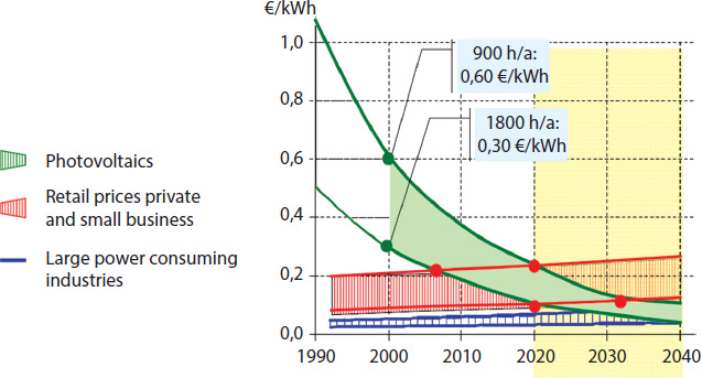
This Figure was also often used when discussing the so called “grid parity”. This is what occurs whenever the PV production cost in different locations (and for a given set of parameters, like WACC (weighted average cost of capital), etc.) becomes equal to the price the various customers have to pay to their electricity provider. As can be easily seen, there is no single point but rather four such intersection points (red dots) spanning an area of different times and locations when this grid parity occurs.

In terms of technology we will see in chapter 6 that there are many different technologies which will evolve for the different market applications, discussed in more detail in chapter 5. The important lesson for PV is that no known electricity generating technology has ever been able to demonstrate such a tremendous cost and price decrease in such a short period of time. This and the modularity of the components of a PV system from kW up to the GW in size will make PV one of the major pillars of the future electricity sector.

I have often heard, especially from economists, that market support programs are not necessary because the market forces will be the best regulator. These people have not understood first, the difference between strategic and consumer goods in a society, and second, the power of technological development associated with lowering the cost and price, if a well-tailored support program is able to provide the increasing cumulative volume of mass produced high-tech products. Both topics will be discussed in Chapter 5.

4.6 Other Renewable Technologies

This section deals with other renewable energy sources, important for the portfolio of a future 100% renewably powered world. We will not discuss these technologies in the same detail as solar, biomass and wind. This is based on the relative importance of the potential contribution within the various renewables as already described earlier in this chapter (compare with Figure 4.1). However, this should not be misunderstood as a dismissal of these technologies as not being important. They will play an important role in regional contributions which have boundary conditions that are very favorable to one of these technologies. But in the author’s understanding, they will not be able to contribute to the 150 PWh challenge as much as the other ones, as will be discussed in more quantitative detail in chapter 9.

4.6.1 Hydropower

There are a good number of countries where conditions are favorable for this type of technology with a well suited landscape and good climate conditions. This enabled them to base a considerable part of their energy needs on the use of hydropower. The Top 10 countries together with the 10 biggest individual hydro power stations are shown in Table 4.6. As can be seen in the case of Norway, up to 98% of a country’s electricity is supplied by hydropower. But also big countries such as Brazil and Canada satisfy a major part of their electricity needs through hydropower.

Table 4.6 Top 10 countries and individual hydro stations as of 2011.

The global historical development of the annual electricity production over the last 46 years was a steady increase, starting with 0.9 TWh in 1965 and growing to 3.5 PWh in 2011 [4-15]. Interestingly, the increase over time was almost linear with approximately 0.5 PWh of additional electricity every 10 years. Let us take an average value of ~4,000 hours of full operational hours per year (calculated from the two stated numbers above: 3,498 TWh/850 GW ~ 4,000 h as a global average). Although this number seems quite low, it takes into account that in many regions the hydro stations cannot operate continuously, especially not in summer time. Combining the numbers indicates an annual increase of ~12 GW new hydro stations. In a publication by Horlacher [4-16] an estimation of the economic, technical and theoretical potential for the global hydro power electricity production was undertaken. The respective numbers are 8.2 PWh, 14.4 PWh and 39 TWh. If we take the same capacity addition for the future as in the past 4 decades, it would take 94 or roughly 100 years to reach the volume given for the economic potential for hydro-electricity. Another estimate was given in terms of price and electricity generation cost, which is summarized in Table 4.7 [4-17].

Table 4.7 Investment and electricity generation cost for different sizes of hydro power stations.

System size	Investment per kW	Electricity generation cost
Up to MW	2.5 – 10 k€	5 – 19 €ct/kWh
Up to 100 MW	1.8 – 6.3 k€	4 – 11 €ct/kWh

The large existing dams and attached power stations contribute the most to today’s hydropower energy. This is normally called “old hydro” as most of these have already been in operation for quite a while. Although there are discussions on new very big hydro plants – for example in Brazil, Africa or Asia – there is growing concern related to the environmental and human damage this may cause. Additional projects like the “Three Gorges dam” in China will become more difficult in the future. It should, however, be remembered that only ~10% of the currently installed hydro power base is accounted for by the very big hydro power plants, as can be seen in Table 4.6. An important contribution to future energy can be made by the so-called “new hydro” which in most cases is a more decentralized power generation with smaller systems. In my understanding, the above stated economic potential of ~8 PWh is the upper limit for hydro energy.

Another important role which hydropower plays and will play in the future is the so-called “pumped hydro”. Many countries like Switzerland are using cheap excess electricity (e.g. base load at night from neighboring countries) to pump water upwards and produce electricity when expensive peak power is needed. As peak power becomes less expensive with more and more PV (and wind) power produced, especially at peak times this business model no longer runs as effectively as in the past. However, for longer term storage this may become an important contribution when excess renewable Energy is to be utilized. Future business models will decide which portion of electricity will be stored using pumped hydro – which does not have high losses – and what that may be compared to the “power to gas” concept, which will be explained later. The latter has high losses originating from hydrolysis (electricity used to produce hydrogen) and converting it back into electricity if needed (by using fuel cells) which amount to roughly 50% losses (assuming about 70% efficiency for both hydrolysis and fuel cell).

4.6.2 Ocean Energy (Wave and Tidal)

Another way of using hydro power is the exploitation of the energy contained in the up- and downward movement of the waves, undersea currents and tidal hubs.

At places with high tide (e.g. Normandy in France with ~8m tidal range, with the spring and neap range as high as 13.5m) there have been attempts for many years to utilize the associated energy streams. One well-known example is the “Rance Tidal Power Station” in Brittany (France) with a 240 MW peak capacity which was completed in 1966. It has a barrage, 750m in length and 13m in height. In practice, the average power is about 96 MW, producing ~ 600 GWh of electricity per year. Interestingly, if we take the total cost in today’s currency and divide it by the total amount of electricity produced, we obtain £3.3 billion / 27.6 TWh =~ 10 €ct/kWh [4-18]. Given the fact that this power station is situated at a very favorable location and all components are in a mature stage, this number shows that the difficulty with this technology is its relatively high generation cost. There is just one more tidal power plant of a similar size in operation today, which was opened in 2011 in South Korea. This plant is called Shihwaho, has a peak capacity of 256 MW and produces ~ 550GWh of electricity per year. Other running tidal plants are much smaller and located in Canada (20MW), China (4MW) and Russia (1.7 MW). There are dreams of a very large tidal power plant in the Bay of Fundy in Nova Scotia in Canada. If this plan could be realized in this place, which has the world’s strongest and highest tides of ~15m, it could generate up to ~2,000 TWh – however, there is no estimate of the cost and the associated electricity generation cost for such a big project.

Instead of building dams, one could also utilize the underwater currents induced by the incoming and outgoing tide. First prototypes are being built and tested and it remains to be seen how durable these turbines will be in the harsh and salty environment, which will ultimately determine the economic viability of such systems. One interesting combination could be the coupling on the same pylon of a slowly moving rotor underwater and a normal operating windmill rotor. This could potentially help to reduce auxiliary costs like mounting structures and electricity network to transport the generated electricity to land.

Pilot projects are also being conducted with systems exploiting the wave energy. Swimming structures are mechanically connected and induce hydraulic pressure by moving up and down with the waves. The size of these pilot projects demonstrates the early stage of this technology, which is in the range of a few MW (like the Agucadoura Wave Farm in Portugal with 2.25 MW which was the first wave farm, started in 2008 and stopped by now).

4.6.3 Geothermal Energy

Geothermal energy utilizes the use of the internal heat of the earth originating from the magma below the earth crust. Magma, which is molten rock, comes to the surface when volcanoes erupt and streams of lava pour out. The basis for this power is the radioactive decay in the Earth’s interior which is estimated to be in the range of 2×10¹³W or 20 TW. Only about 40 to 80 mW/m² reach the surface which is only a tiny fraction (<10⁻⁴) of the 1 kW/m² coming from the sun at normal incidence at peak solar radiation (or 100 to 250 W/m² continuous calculated average power). In some regions – Yellowstone Park, Iceland and many more places – hot water springs can be used to heat houses. The normal situation, however, is a constant temperature of between 10°C and 16°C in the shallow ground reaching the surface.

Table 4.8 Carnot efficiencies “Eta” for various inlet temperatures at fixed low temperature at 25°C (T measured in Kelvin = 273 + x°C).

Once a geothermal power plant is up and running it continuously produces electricity which can be used for base load applications. Although the running cost is rather low, there are, however, important restrictions.

• high cost of drilling
  Depending on the geological formation, the cost of drilling the necessary holes is rather high and a major component for the generation cost for this technology. In a German ministry (BMU) study [4-19] the cost for a 5km borehole was estimated at €4 million.
• Low Carnot efficiency
  As the inlet temperature to the turbine is generally low in the range 200°C, the Carnot efficiency is also rather low. This leads to the fact that the specific investment cost for the conventional part for this type of electricity generation – steam generation, turbine, cooling tower – is rather high. For comparison, the Carnot efficiencies for a range of inlet temperatures are summarized in Table 4.8. Note that an inlet temperature of 150°C has only half of the efficiency of a state of the art turbine fired by fossil or nuclear produced steam.

Combining the different input parameters leads (with an investment cost of ~(2.5 – 5) k€/kW and 8,000 full load hours per year) to an electricity generating cost of (7 – 15) €ct/kWh.

4.6.4 Heat Pump

The utilization of surrounding heat (air or soil) with heat pumps requires a considerable portion of external energy. According to a study by the German ministry BMU [4-20], heat pumps can be called hybrids between saving conventional energy usage and renewable Energy. To provide the same 100 kWh heat for a household, a comparison was made between a standard caloric value burner, an electricity driven heat pump, and a gas motor driven heat pump. While for the classical gas burner 112 kWh’s are needed, the corresponding numbers for the electricity (using primary energy numbers) and the gas motor driven heat pump are 78kWh and 66kWh, respectively. It is interesting to see that at the time the study was conducted in 2004 the examples given for various external energy inputs did not recognize that if electricity was provided by renewables then this device was no longer a hybrid but a 100% renewable device. If we only take into account the secondary energy, then the electricity driven heat pump needs only 26 kWh, making renewable electricity the most efficient way of powering a heat pump. There is also the misleading guideline as to which “coefficient of performance” (COP) for an electrical heat pump should be used. This COP is defined as “useful heat/work input”, which for our above example is 100/26 ~ 4 using secondary energy numbers for electricity, but only 100/78 ~ 1.3 when using primary energy data. For conventional electricity, the “work input” in form of primary energy is 3 times higher due to losses in the power station, therefore it is normally recommended that this COP for electrical heat pumps should be higher than 3, while for gas engine driven heat pumps it only has to be above 1.1. With renewable electricity, the same lower limitation should be applied.