CHAPTER 3

The Role of Machine Learning on Future of Work in Smart Cities

Ammar Rayes

Abstract

Digitization, or the Fourth Industrial Revolution,1 is driven by automation and information technology. It is causing massive market disruption in the job market regarding the future of work as machines are able to perform tasks better than human beings and are able to communicate with other machines to take the appropriate action. These machines are enabled by recent disrupted technologies including:

• Cloud Computing and Virtualization: Cloud computing allows companies to outsource their computing infrastructure fully or partially to public cloud and saves the cost of hosting all of their compute applications in a private data center. Recent data showed that the average network computing and storage infrastructure for a startup company in 2000 was $5 million. The cost in 2016 had dropped to $5000. This enormous 99% decline in cost was made possible by cloud computing [2].
• Internet of Things (IoT): IoT is defined as the intersection of things (e.g., sensors), data, Internet, and standardized processes across multiple industry verticals. It allows machines to sense information at any time and communicate with other machines inexpensively and in real time.
• Big Data: Big data refers to extremely large structured and unstructured data sets that are difficult to analyze in real time with traditional data processing or computing systems. It is referred to as data with three “high Vs”: high volume, high velocity, and high variety. Big data systems allow machines to analyze massive amounts of data and to produce intelligence in near real time. Companies are interested in big data applications to analyze extremely large data sets to reveal patterns, trends, and associations, especially relating to their customer behavior and buying patterns.
• Advanced Wireless Networks: Wireless networks are computer networks that use wireless data connections between network nodes. Wireless networks include licensed cellular network and unlicensed noncellular networks (e.g., WiFi, LoRa) allowing IoT and other devices to connect to the network and communicate.

At the top of the technology enablers are Artificial Intelligence (AI), Machine Learning (ML), and Deep Learning (DL). AI/ML/DL may be considered as the brain of the overall system, as shown in Figure 3.1, with a job to make intelligent decisions.

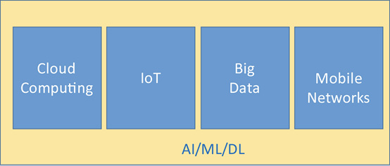
Figure 3.1 Relationship between AI/ML/DL and fourth industrial revolution technologies

Business leaders across the industry are convinced that AI/ML/DL can add significant value to their environment, bring efficiencies, lower their operating costs, and increase their market share. At the same time, the vast majority of such leaders are not sure where to start. One thing they’re keen on is hiring experts with AI/ML/DL background.

This chapter first introduces AI, ML, and DL, and then provides use cases for the IT industry.

Artificial Intelligence, Machine, and Deep Learning

Artificial Intelligence (AI)

Artificial Intelligence (AI) is the overall concept of machines being able to perform useful tasks that a human being typically does, i.e., “intelligence of human being reproduced by machine.”

AI was founded in the 1950s as an academic discipline and has experienced several waves of optimism since then. For instance, in the late 1960s, Marvin Minsky and Seymour Papert of the MIT AI Lab used AI in conjunction with various colors and blocks of various shapes and sizes to simplify the illustration of physics and sciences. They felt that physics and sciences were best understood by using simplified models like frictionless planes or perfectly rigid bodies [3]. In the early 1980s, Danny Hillis, a recent MIT graduate, enhanced AI by introducing the connection machine by utilizing parallel computing, a type of computation in which computation tasks are broken down into many smaller tasks and then carried out simultaneously [4]–[5]. The results are subsequently combined upon completion.

AI is used in object recognition, speech recognition, speech detection, natural language analysis, and painting creation, which are techniques for restoring or transforming parts of translations, missing parts from the whole.

Machine Learning (ML)

ML is a main application of AI and is based on the concept that “just give machines access to data and let them learn for themselves” for the purpose of predicting things correctly. ML can be defined as the ability for a machine to learn from data with data, without being explicitly programmed to perform a specific task.

ML involves teaching a computer to recognize patterns by examples, rather than programming it with specific rules. Hence, ML creates algorithms or rules from data and make predictions on them.

Deep Learning (DL)

DL is part of a broader family of ML methods based on learning data representations, as opposed to task-specific algorithms. Learning can be supervised, semisupervised, or unsupervised as we’ll show later in this chapter. Figure 3.2 illustrates the relationship between AI, ML, and DL.

Figure 3.2 Relationship between AI, ML and DL

It should be noted that the terms AI and ML are often used interchangeably especially by inexperienced users in generic industry.

ML Algorithm Categorization

This section breaks down ML algorithms into common categories and then lists the corresponding algorithms in each category. Specific examples will be provided in the next section. Given the large number of algorithms, we’ll not be able to explain the details of each algorithm. We’ll advise, therefore, that the reader reviews a basic technical ML book and/or takes a training course online if needed.

In general, ML can be divided into three main categories: supervised learning, unsupervised learning, and reinforcement learning as shown in Figure 3.3.

Figure 3.3 ML algorithm categorization

Supervised learning includes regression and classification techniques. Top examples of regression algorithms include: linear regression, support vector regression (SVR), Gaussian processes regression (GPR), ensemble methods, decision trees, and neural networks. Top examples of classification techniques include support vector machines, discriminant analysis, Naïve Bayes, nearest neighbor, and neural networks.

The main area of unsupervised learning is clustering. Top clustering techniques include: K-means, K-medoids, hierarchical, Gaussian mixture, Hidden Markov model, and neural networks. Both K-Means and K-medoids are partitioning clustering techniques that cluster the data set of n objects into k clusters with k known a priori. The K-medoids method is considered more robust to noise and outliers.

Reinforcement learning algorithms include Q-Learning, Sarsa2 (an On-Policy algorithm for Temporal Difference Learning), and Deep Q-Networks [13]. The major difference between Sarsa and Q-Learning is that the maximum reward for the next state is not necessarily used for updating the Q-values.

Some readers may be asking by now what are neural networks and why do they appear in every ML category? Well, neural networks are systems patterned after the operation of neurons in the human brain. They “learn” with examples, generally without task-specific programming. For example, “neural networks might learn to identify images that contain people by analyzing example images that have been manually labeled as “people” or “not people” and use the results to identify humans in other images. They do this analysis without any a priori knowledge about human, e.g., that they have two legs, two arms, a face with two eyes, two ears, a centered mouth, a nose, and human-like faces. Hence, neural networks evolve their own set of relevant characteristics from the learning material that they process [10].

Smart City Applications

Linear Regression

Linear regression is a simple approach for modeling the relationship between a scalar variable “y” and one or more explanatory variables “x”. Hence, “x” is regarded as the descriptive independent variable and “y” is the outcome or dependent variable.

To establish a relationship / hypothesis, we place the independent variable on the x-axis and the dependent variable on y-axis and then try to find the best relationship between “x” and “y” variables with a straight line. As the independent variable “x” changes, the behavior of the dependent variable “y” is tracked with a sufficient number of observations3 before the line is drawn.

Linear regression is often used in smart city applications to predict forecasting. For example, let’s assume that we are trying to predict traffic congestion levels (e.g., 0–100% where 0 indicates nil congestion and 100% indicates a complete traffic jam) in a smart city as temperature changes. The first step is collecting data (x = temperature and y = traffic congestion level) over an adequate4 period of time. Next, the collected data is divided randomly into two datasets: dataset 1 and dataset 2. Dataset 1 is used to plot the regression line (or hypothesis) and dataset 2 is used to verify that the regression line is placed correctly (or the hypothesis is correct), as shown in Figure 3.4. If the hypothesis is correct, then the regression line is assumed to be valid and may be used for future prediction. If not, then a new line should be drawn perhaps after collecting additional data.

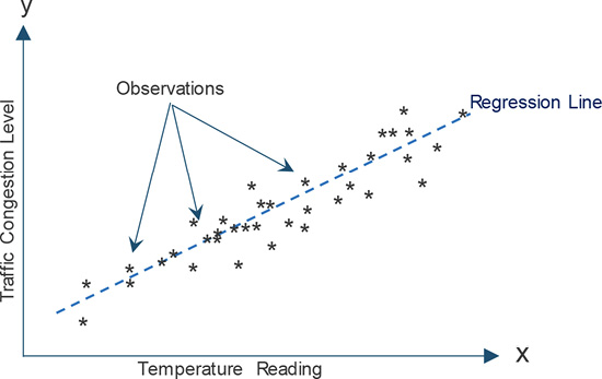
Figure 3.4 Liner regression example

It is important to note the following:

• Even if the model is correct for every point in dataset 2, there is no guarantee that the same model will always be correct for future data points. There are techniques in statistics to predict the predictability of certain events such as “entropy,” which measures the amount of uncertainty or randomness in data. For example, the entropy for a fair coin is quite high (e.g., there is no way of determining what the outcome of the next toss even if the last 10 tosses show 3 heads and 7 tails) whereas the entropy of a coin with two heads is zero (the outcome is certain). This example illustrates the importance of collecting sufficient data.
• As stated earlier, the observed data should be always divided into two parts. One part (i.e., the large part, denoted as dataset 1 previously) should be used to construct the regression line (hypothesis) and the other part (dataset 2) should be used to validate the hypothesis (why this is important).

Decision Tree

Decision trees are also common machine learning techniques that are relatively simple to use and illustrate. They are used to explicitly represent decisions using branches (each branch represents a decision or an outcome) and leaves (each leaf node holds a class label). A decision node has two or more branches.

Cities around the world have been deploying sensors to measure temperature, wind speed, pollution, noise level, etc. IoT sensors are considered constrained devices (i.e., they have limited power and data processing capabilities) and often are placed in the open within a rough weather environment. Hence, sensors may fail and start reporting wrong information over a period of time.

In this example, we would like to build a model that predicts if an abnormal value is an indication of a problem (e.g., air pollution is too high) or if it is a “faulty reading” of the sensor. From history, we know that sensors fail due to their age, quality/brand (we’ll track by the manufacturer and product identification (PID)), weather conditions (i.e., they may report wrong reading if the sensor is wet), wind conditions, and possibly other criteria.

Let’s assume we collect the following data for a sufficient period of time (e.g., one year):

• Date and time
• Sensor’s manufacturer: Vendor’s name, PID
• Sensor’s age in years
• Weather outlook: sunny, rainy, or overcast
• Wind conditions: strong or weak

Let’s also assume that we take the “Sensor Data” as the first main attribute. The two subattributes of interest are then the sensor’s PID (assuming that we have a list of faulty sensors based on PIDs) and the sensor’s age (assuming that collected data showed that the sensor’s quality degrades rapidly).

Now, assume that we observed a large number of faulty readings during high winds. Hence, we’ll take the Wind Condition as the second main attribute. Finally, we’ll take the Weather Outlook as the third and final attribute (Figure 3.5).

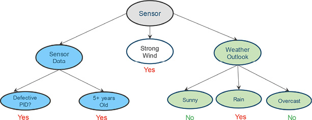
Figure 3.5 Decision tree: Prediction model for defective sensors

In general, attributes should be split further if the historical data did not provide confident answers with high probability. For example, we did not need to split the “Strong Wind” attribute further as the collected data consistently showed that sensors reported “faulty readings” during strong wind. On the other hand, if the historical data did not provide a confident answer, then additional subattributes should be added (e.g., “strong wind with rain” and “strong winds without rain” assuming the data is accurate when both “Strong Wind” and “Rain” conditions are tracked at the same time).

Based on the previous model, one can predict when a new sensor reading is wrong, that is, “Strong Wind” results in “fault reading” with very high probability (purely based on historical data).

Finally, in decision trees, it is a good idea to track the counts of positive and negative predictions at each node and use such data to build a confidence model. For example, assume that the data we collected so far consisted of 1000 measurements with 600 positives (i.e., correct faulty readings) and 400 negatives (incorrect fault readings) before any splitting. At this stage, 600/400 may be placed on the top of the “Sensor” node as shown in Figure 3.6 Now, let’s assume that 323 readings in total were captured during “Strong Winds” with 310 positive and only 13 negative readings. Further data is illustrated in the figure. It should be noted that the confidence numbers should be updated as more data is collected. The addition of more data will of course result in better confidence.

Figure 3.6 Decision tree with confidence—Prediction model for defective sensors

6.3 K-Means Clustering Unsupervised Learning

K-means clustering aims to partition n observations into k clusters in which each observation belongs to the cluster with the nearest mean. This example focuses on optimizing energy usage in smart city data centers using K-mean clustering.

Smart city (or government) data centers generally consist of a large number of servers (physical machines (PMs)) that are grouped into multiple clusters. Each cluster manages and controls a large number of PMs. The centers offer computing services for various branches of government and agencies (called clients) and may charge them based on their usage. Clients submit requests to the data centers, specifying the amount of resources they need to perform certain tasks. Upon receiving a client request, the data center’s cluster scheduler allocates the demanded resources to the client and assigns them to a PM. The virtualization technology allows the scheduler to assign multiple requests possibly coming from different clients to the same PM. Client requests are thus referred to as virtual machine (VM) requests.

With the “Green Initiative,” energy optimization is very important to smart city’s government and data center providers. It is important, therefore, to put servers to sleep when they are not in use. To do so, we have developed a novel technique to monitor PMs and effectively decide whether and when they need to be put in sleep mode. The solution framework has three major components: data clustering, workload prediction, and power management. A more detailed explanation of this solution is provided in the references [14]. In this example, however, we’ll focus on how data clustering is utilized.

K-means clustering is used to create a set of clusters by group VM requests of similar characteristics (in terms of their requested resources) into the same cluster. Each VM request is mapped into one, and only one, cluster. The solution is evaluated using real Google traces [15] collected over a 29-day period from a Google cluster containing over 12,500 PMs.

The K-means algorithm [16] assigns n data points to k different clusters, where k is the a priori specified parameter. The algorithm starts by an initialization step where the centers of the k clusters are chosen randomly, and then assigns each data point to the cluster with the nearest center (according to some distance measure). Next, these cluster centers are recalculated based on the current assignment. The algorithm repeats by assigning points to the closest newly calculated clusters and then recalculates the new centers until the algorithm converges [15].

Figure 3.7 shows the resulting clusters for k = 4 based on the training set, where each category is marked by a different color/shape and the centers of these clusters c1, c2, c3, and c4 are marked by “x.” Category 1 represents VM requests with a small amount of CPU and a small amount of memory; Category 2 represents VM requests with a medium amount of CPU and a small amount of memory; Category 3 represents VM requests with a large amount of memory (and any amount of requested CPU). Category 4 represents VM requests with a large amount of CPU (and any amount of requested memory.). Observe from the obtained clusters that requests with smaller amount of CPU and memory are denser than those with large amounts.

Figure 3.7 The resulting four categories for Google traces using K-means clustering [14]

Conclusion

We’d like to conclude this chapter by restating the definition of AI, ML, and DL. AI is the overall concept of machines being able to perform useful tasks which a human being typically does, that is, “intelligence of human being reproduced by machine.” ML is a main application of AI and can be defined as the ability for a machine to learn from data with data, without being explicitly programmed to perform a specific task. DL is part of a broader family of ML methods based on learning data representations, as opposed to task-specific algorithms. Learning can be supervised, semisupervised, or unsupervised.

This chapter introduced the main emerging technologies, namely cloud computing and virtualization, IoT, big data, and advanced wireless networks, coupled with AI/ML/DL. Next, the impact of the overall solutions on the future of work was shown. Three very specific smart city ML examples were provided in the areas of linear regression, decision tree, and K-means clustering unsupervised learning.

References

Schwab, K. 2016. “The Fourth Industrial Revolution: What it Means, How to Respond.” World Economic Forum Report, January 14, https://weforum.org/agenda/2016/01/the-fourth-industrial-revolution-what-it-means-and-how-to-respond/

Rayes, A., and S. Salam. December, 2018. IoT from Hype to Reality, the Road to Digitization, 2nd ed., Springer.

Artificial Intelligence and Machine Intelligence, Wikipedia, https://en.wikipedia.org/wiki/Artificial_intelligence#Probabilistic_methods_for_uncertain_reasoningc

Morgan, July 2018. “Machine Learning Is Changing the Rules.” O’Reilly Media, Inc, https://oreilly.com/library/view/machine-learning-is/9781492035367/

History of AI: https://en.wikipedia.org/wiki/History_of_artificial_intelligence

Kanter, R.M. November 2011. “How Great Companies Think Differently.” Harvard Business School, Issue: https://hbr.org/2011/11/how-great-companies-think-differently

Lemonlck, S. August 27, 2018. “Is Machine Learning Overhyped?” Computational Chemistry 96, no. 34, https://cen.acs.org/physical-chemistry/computational-chemistry/machine-learning-overhyped/96/i34

Chollet, F. December 22, 2017. Deep Learning with Python, 1st ed., Manning Publications, ISBN-13-078-16117294433

Harris, R. 2016. “More Data will be Created in 2017 than the Previous 5,000 Years of Humanity.” App Developer Magazine, December 23, 2016. https://appdevelopermagazine.com/more-data-will-be-created-in-2017-than-the-previous-5,000-years-of-humanity-/

AI Neural Network, Wikipedia: https://en.wikipedia.org/wiki/Artificial_neural_network

Tiwari, S. Face Recognition with Python, in Under 25 Lines of Code, https://realpython.com/face-recognition-with-python/

Time Eden, Anthony Knittel and Raphale V. Uffelen, Reinforcement Learning Tutorial Online.

Quoc V. Le. 2015. “A Tutorial on Deep Learning, Part 2: Autoencoders, Convolutional Neural Networks and Recurrent Neural Networks.” October 20, http://citeseerx.ist.psu.edu/viewdoc/download?doi=10.1.1.703.5244&rep
=rep1&type=pdf

Dabbagh, M., B. Hamdaoui, M. Guizani, and A. Rayes. September 2015. “Energy-Efficient Resource Allocation and Provisioning Framework for Cloud Data Centers.” IEEE Transactions on Network and Service Management,: http://web.engr.oregonstate.edu/~hamdaoui/papers/2015/mehiar-TNSM-15.pdf

Google Data Center Data Traces, November 2011. http://code.google.com/p/googleclusterdata/

Han, J., M. Kamber, and J. Pei. 2011. Data Mining: Concepts and Techniques, Morgan Kaufmann.

---