CHAPTER 6

Designing a Rate-Based Planning Process

Rate-based planning (rbp) is a significant departure from conventional S&OP and the conventional scheduling practices of MRP (material requirements planning), as imbedded in all ERP (enterprise resource planning) systems. Using RBP can have a transformational impact on your business, increasing cash flow and delighting your customers with excellent service.

MRP, JIT, and the so-called pull systems that ERP has added all start the production process when a new order comes in and trips a replenishment signal, either a safety-stock level or a Kanban trigger. This trigger is not limited to any capacity consideration, nor is it sensitive to order trends; it just starts new production even when the trend would say you have enough already. In RBP, you use expected order rates, as determined in S&OP, to gauge whether a series of orders are as expected. When the rate of incoming orders is higher or lower than expected, you reexamine the situation and determine whether you want to change the master schedule. Most often, you will wait for further information before changing the schedule. This is the principle of “don't make a decision until you have to.”

These two guiding principles are the basis of rate-based scheduling:

 

1. Build to an order rate, not to an order.

2. Don't make a decision until you have to.

Chapter 6 describes the applicability of RBP, the history of scheduling schema, and the process tools and key elements of RBP.

RBP Applicability

RBP can be applied to almost all manufacturing businesses, the true job shop being the most notable exception. However, only a very small portion of manufacturing is truly job shop. MRP, safety stocks, and forecasting still are necessary in scheduling capacity-constrained job-shop operations. However, RBP is the proper scheduling tool for the type of job shop in which extensive use of cellular manufacturing is in place.

RBP schedules production to demand—true demand, not the demand surrogates that come in the form of replenishment orders from upstream stocking locations or from forecasting. Before all the forecasters go crazy, forecasting still is used for longer-range (12 to 18 months or more) capacity planning. RBP plans to the end-user take-away rate. For manufacturers that sell through distributors, this is not distributor stock replenishment orders; it is the actual purchases of end users such as OEMs (original equipment manufacturers). For those manufacturers that sell to retailers or brokers, it is the rate the retailers sell to consumers, not the rate of replenishment to retailer distribution centers. For medical device manufacturers, demand is the number of devices used in surgical procedures, not the shipments to consignment stock or to distributor safety stocks.

RBP works for both make-to-order (MTO) and make-to-stock (MTS) businesses. The preference would be to convert an MTS business to an MTO one by reducing the master-schedule horizon to a few days and producing very close to the actual consumer take-away rate and mix. In some businesses, particularly consumer products or food manufacturing, MTS is probably required. However, you still replace short-term SKU-level forecasts and safety stocks with family-demand rates and inventory balancing. The objective in both MTO and MTS situations is to eliminate or drastically reduce finished-goods inventory and to use manufacturing flexibility to produce to true demand. Ideally, you eliminate not only your own finished goods inventory but also the inventory in distribution, except for goods in transit or being cross-docked. Certainly, some companies have seasonality-forced capacity shortages. In those cases, RBP would have a prebuild strategy resulting in some finished-goods inventory. In the prebuild strategy, you use a zero-zero inventory strategy, committing only the inventory guaranteed to sell during the season and leaving open the ability to adjust production to actual demand for a substantial part of the season.

In an MTO business, the RBP process manages variability in demand by managing order backlog, rather than inventory safety stock. This is not new to highly engineered MTO businesses. What is new is operating as an MTO business in traditional MTS situations. We have converted food manufacturers to MTO, as well as medical technology businesses, consumer durable businesses, and commercial products companies.

In an MTS business, the RBP process has a totally new inventory replenishment strategy. Rather than produce to replenish stock at a location when the individual-item forecast predicts a safety-stock violation, RBP selects an SKU mix each time a family is to be produced, such that a balanced inventory results. In RBP, you produce the items with the highest probability to sell in the very near term.

RBP Versus Traditional Scheduling Methods

RBP is a pull process. Many managers think they are using a demand-pull process, because demand pulls inventory down. If inventory initially was put in place to a forecast (which is a push concept) and is maintained using safety stocks calculated from a forecast (another push process concept), you do not have a pull process. In RBP, you set the expected rate of capacity usage to a highly accurate aggregate forecast of all members of a 3M family. The rate comes from the monthly collaboration, but you actually make to the mix and volume of true demand. There are no individual SKU forecasts at all—none—and there are no safety stocks. In cases in which manufacturing cannot produce to true demand inside customer lead times, you calculate an inventory standard, which is a range of acceptable inventory but does not work as a safety stock, only as a balancing factor. All items within a family should have the same stocking level in days of supply at the end of a family production run.

RBP Supports the Time-Advantaged Strategy

I introduced RBP in Chapter 2 as the method required to support a time-advantaged strategy; that is still true. However, RBP has a much broader applicability and is far superior to the traditional scheduling methods commonly used and included in supply chain software. Figure 6-1 shows how RBP differs from traditional methods of scheduling at the concept level.

MRP is the Push System Inside ERP

The MRP process was defined in the 1960s, as computers were just starting to be applied to manufacturing. It has stayed in the software designers’ application set through many upgrades, but it stays the same. All MRP applications are designed for a true job shop. ERP systems of the 1990s and the MRP II, MRP, and PICS (production and inventory control system) systems of the 1970s and 1980s were written by computer programmers who simply copied the scheduling concepts designed in the 1960s for the job shop. The “modern” ERP is just a copy of what the pioneers at Warner & Swasey Company and The Stanley Works came up with in their job-shop applications. In fact, in the late 1960s, I was a member of the teams designing the systems for Warner & Swasey (W&S), which was the ultimate job shop. IBM's PICS system came directly from the work we did at W&S. Later, the Arista System was adapted directly from the W&S system. Since the 1960s, the logic for scheduling in MRP has not changed significantly. MRP is widely accepted as the way to schedule any and all types of factories, even though we knew from the very beginning that it applied only to job shops. One significant group of manufacturers did not accept MRP: The leading Japanese manufacturers use a very primitive form of rate-based processing that employs Kanbans to accomplish the demand-based signaling that MRP is incapable of producing.

FIGURE 6-1. COMPARISON OF SCHEDULING SCHEMES BY DECISION-MAKING PRIORITY.

RBP optimizes inventory and maximizes throughput; both produce free cash flow.

MRP was designed to explode the bill of material for an assembled product into individual parts. The parts were then planned over a lead time to be produced in time to be available for the assembly operation. Assembly was planned using an S&OP process in an MTO environment. MRP ignores capacity constraints completely. Supposedly, the assembly master schedule was developed to allow for capacity constraints, but in the job-shop environment, individual parts compete for capacity on feeder production equipment, so it is very difficult to predict capacity usage. Elaborate finite scheduling processes were developed to deal with the problem and were successful to some degree. All is well with this approach.

However, when the so-called independent demand problem was presented to the MRP designers, the scheduling problem became complex. Demand for individual parts came from customers, as well as from the assembly schedule. The MRP designers tried to add independent demand forecasts to the exploded expected requirements from the assembly schedule. In a job shop, lead times for parts are very long. Forecasts over long horizons typically are very inaccurate, so as the actual demand came in and was different from the forecast, major schedule changes happened. The schedule changes continued—and continued to be magnified. This problem was even named back in the 1970s as the “bullwhip effect.” The solution was to add large safety stocks and to try to develop the “perfect forecast.” The only economic benefit of this historical struggle fell to software manufacturers, which were and are rewarded for providing ever-more-complex and costly MRP software, forecasting software, etc. Manufacturers gained high inventory and high obsolescence. The big failings of MRP are poor cash flow and the inability to plan collaboratively. MRP is driven by the drum of forecast error, not the demand rate of S&OP.

Managers decided to put in pull processes to stop the tyranny of MRP. This was a good idea, but it was poorly implemented. It was interesting to see all the software companies almost instantaneously offer a pull-process application in the 1980s. All they did was dress up MRP.

In time, a pull process called just-it-time (JIT) was developed. The origin of JIT was the popularity in the 1970s of the Toyota Production System (TPS), with its Kanbans and pseudo-pull processes. One large consulting firm purported to know how the TPS worked and could be applied widely. The firm was paid large sums of money, but it rarely had a successful installation. The problem in applying the TPS is that auto manufacturing is very simplistic, while the vast majority of manufacturing is much more complex. Toyota makes one product in each plant, a vehicle, with a set manufacturing rate determined in large part by the design of the factory. If the factory is designed for 35 cars per hour, then it produces exactly 35 cars per hour. In Toyota's case, the company offered very few options or only a standard option package, so predicting the demand for parts was much easier. The Kanban signaled for replenishment only when small variations in the rate changed the supplier schedules very slightly, so the process worked with low inventory. The problem comes in when a company's manufacturing does not mirror the Toyota model.

JIT is a Push System Inside a Make-to-Order Manufacturing Design

JIT tries to minimize inventory to the exclusion of all other factors or goals. In practice, JIT does two things, both of which are counterproductive. First, the manufacturers that employ JIT as a scheduling strategy end up with massive amounts of excess capacity. JIT says anything, anytime, and any quantity. Only the most simplistic manufacturing operations could possibly do this. These would include some manual assembly operations, with flexible workforce characteristics and very limited capital equipment requirements. Second, the manufacturers using JIT for supply force inventory downstream to suppliers. They have the least possible chance of producing to true demand, and thus, end up with massive amounts of inventory, which leads to higher costs, higher prices, and eventually may cause bankruptcy. Sometimes, these supplier-JIT arrangements are called vendor-managed inventory, or VMI. This is interesting phrasing, as the word “vendors” calls to mind people who sell hot dogs on the streets of New York, not critical business partners. Manufacturers that try to work with major retailers through an arms-length VMI process—typically managed by the sales department, where there are no inventory management skills—become frustrated and end up with large inventories, massive manufacturing schedule changes, and very high costs relative to other non-VMI customers. The excuse is “we will make it up in the volume,” but of course they cannot.

In the big picture assessment, neither JIT nor MRP are collaborative processes. They do not work within the capacity as defined by S&OP, and they do not signal when planned capacity is being exceeded or is unutilized. Both exaggerate the peaks and valleys of demands on capacity by overreacting to short-term demand variations that should be ignored. They are anathema to an efficient and effective market-driven process. Demand is variable and S&OP, along with RBP, deals with the demand variability effectively. Any scheduling scheme that builds inventory and/or requires excess capacity is not optimal.

The other major problem with MRP and JIT is that they operate at a highly detailed level and way into the future. MRP deals with individual components for every product, all the time, and so does JIT. Consider the problem of ‘C’ items. (Note that to keep the problem simple, I have only ‘A’ and ‘C’ items in my definition of the way the world works. Some people follow a strict Pareto distribution, with its ‘A,’ ‘B,’ and ‘C’ items; I find this much too complex. I even had a client who used ‘A,’ ‘B,’ ‘C,’ ‘D,’ and ‘E’ items. Using an ‘A’ and ‘C’ item definition is sufficient.)

‘C’ items are 80 percent of the finished goods items, but only about 20 percent of the total throughput. In MRP and JIT, all items are dealt with as if they were equally important. Since ‘C’ items have significantly more volatility, they trip a replenishment signal much more often than their 20 percent would indicate. They totally consume your time because the sheer number of them is overwhelming. Literally every day, a mess of ‘C’ items have orders come in differently than expected, and the MRP or JIT responds by triggering production. In practice, schedules are chaotic. Employees who work down in the plant and deal with MRP every day know exactly of what I speak. Unfortunately, they are shouted down by the IT wizards and senior managers who spent millions of dollars on “the system” and are emotionally wed to it, even if it does not work.

My advice is to throw MRP out, stop thinking about JIT, and install an RBP process without delay.

RBP Scheduling Strategy

The remainder of Chapter 6 is for companies that have significant setup time or line-change time. Even if you are able to become almost MTO using Lean or Six Sigma, and matching the manufacturing lead time to the customer's need, you will need the tools described in the following sections. Some companies can have dedicated production lines and can make whatever is required every day; the beverage manufacturers were like this until they exploded their product offerings tenfold. So, almost all manufacturers that are not true job shops will benefit by using RBP tools.

As I pointed out in the introduction to this chapter, the basic principles are building to rates and not making decisions until you have to. In RBP, super ‘A’ items or order backlog become the buffers to variation in demand, not safety stock on all items and not safety stock on the super ‘A’ items.

The strategy for scheduling in RBP is to use capacity to make what will sell in the near term. That is, make those ‘A’ items that have the least amount of demand variability. This is a new concept for most managers. ‘A’ items normally are defined by a Pareto ranking of sales revenue or some other volume-related factor. Some managers even use item sales value, i.e., the most expensive items are the ‘A's. Both of these methods to define ‘A’ items are of little use here. The ones you want to commit to stock when you don't have actual demand information are the ones with the lowest variability, the most stable items. The idea is to conserve capacity. If you make high-volatility items, you risk having put up finished goods that will sit in inventory. In that case, you have wasted capacity on something you did not need right away, made it before you had to, and have no scheduling buffer from those items. If you make low-volatility items, you can be assured of having demand tomorrow that can be satisfied from already-produced items, and thus, you have capacity available for the items actually in tomorrow's demand mix.

Let's look at an example:

There are 300 items in the family.

Some 20 items equal 50 percent of total demand and are in the actual demand mix almost every day.

As a group, they account for a minimum of 30 percent and maybe as much as 70 percent of every day's actual demand.

You can then make some of these 20 super ‘A’ items into finished goods.

You schedule capacity for this family to the aggregate average daily demand. The accuracy of your estimate of average daily demand is high, because it is at a relatively high level of aggregation. However, you can deal with some volatility in the daily family demand, as you will see later in this chapter.

On days when the actual demand is below the aggregate average, you fill up the production to planned capacity with the super ‘A’ items in the worst stocking position (worst will be defined using inventory standards, discussed below).

On days when the actual demand is higher than the aggregate, you make all the non-super ‘A’ items in the actual demand mix and satisfy the excess demand from the stock of the super ‘A’ items built previously.

By following this strategy, the peaks and valleys of production are eliminated, and ‘C’ items are made when they are required, without disturbing the overall production allowance for the family.

‘C’ Item Strategies

If ‘C’ items are too much of a problem to handle in daily production within a family, or if they have their own families because of raw material issues (which is often the case), you want to eliminate their impact by simply making a quantity of three to six months’ supply early in the overall production cycle (an annual cycle or the seasonal cycle for the product line).

I don't like to make ‘C’ items in more than about three- or four-month quantities because of the demand variability. Three months may become eight months or a year very easily as a result of the inherent error in future planning.

When significant setup or line-change time is involved, you should try to batch the ‘C’ items in an off-season period or in the low production months.

Another ‘C’ item strategy is to reserve capacity for ‘C’ families in the cycle plan, which we discuss next.

Cycle-Plan Strategy

When setup is significant and many different families are made on the same production line, a cycle plan is used to implement the RBP process. Cycle plans have a horizon of two to three weeks at maximum, and perhaps only two or three days, as is the case in many food-processing businesses. Cycle plans show what family is made during each shift of each day. ‘C’ families can be grouped together and scheduled for about 20 percent of the normal capacity, or about one out of five days per week. Cycle plans are updated once a week or perhaps more frequently. On the update day, the ‘C’ families that have the lowest number of months of supply are chosen for production. The total production is whatever 20 percent of the week's capacity is planned to be. Then, if the ‘C’ families as a group start to trend so that they have more than the planned months of supply, you skip making ‘C’ families for one week. If the ‘C’ families start to drop below a few months of supply and threaten stockouts, you may want to add a half-day or so in the next cycle plan.

Some people worry about ‘C’ items within an ‘A’ family or ‘C’ families with very long lead-time components. Normally, these are not a problem. You can either stock the long-lead component if it is not too expensive and has a long shelf life, or more likely, you keep a little more than three months’ worth on hand, so when the long-lead item is found to be needing more production, you have time to add it to the cycle plan a few weeks forward, without creating a stockout. If the ‘C’ item is not really that important overall, consider getting rid of it altogether.

In job shops, cycle planning is used to manage the capacity-limited operations. Take a printed circuit board (PCB) operation, for example. The PCB plants make double-sided boards and multilayered boards. The double-sided and multilayer PCBs use drilling capacity, which is an expensive and capital-intensive part of the operation. Multilayered PCBs use more drilling than double-sided PCBs by a multiple of two to three times. So, the planner must feed new orders from backlog to match the available drilling capacity. The cycle plan comes in when deciding the mix of double-sided and multilayered PCBs each day. The inner layer department (the area of the factory where the multiple layers of circuits inside a multilayered PCB are aligned and assembled) is also expensive due to the need for highly trained staffing. The department may not be staffed every day, so the orders for multilayered PCBs must be released to production inside the restrictions of the cycle plan. If the backlog of multilayered boards builds, more shifts of inner layer department capacity must be added and vice versa.

In food manufacturing, the filling lines run to one cycle plan, and the labeling lines run to a second cycle plan. The inventory available for labeling is not known in detail until the production in filling is completed and the mix of individual items is known to labeling. Because labeling may take place several days after filling, allowing for incubation time in quality control, the actual demand for each labeled item is determined at the future date, not before. In labeling, you often have not only different brand labels but different packaging configurations, from six packs to cases, and so on.

Zero-Zero Inventory Strategy

The term “zero-zero inventory strategy” comes from a technique I first learned from Harry Figgie, the CEO of the parent company of Rawlings Sporting Goods Company, the first zero refers to rebalancing production to demand early in a season to zero at the end of the season and the second zero refers to doing the rebalancing again later in the season when demand for the total season can be projected more accurately. The idea is to have zero inventory carryover at the end of the season.

Often we find a business has a natural seasonality or promotional activity. Both situations present the opportunity to employ a zero-zero inventory strategy. Some managers do not think about seasonality because they are in a hard-goods business, but many businesses actually have an off-season, and thus, a beginning of a new season. Some businesses have a natural or customary time of the year when product-line changes are introduced, so there is a beginning and an end to the cycle every year. Businesses that have production in, say, China, with very long transit times, may need to be committing production far ahead of actual demand. The zero-zero strategy works exceptionally well in these cases. This strategy can also be applied to new product introductions when the business does not have a customary introduction period and launches new products whenever they are ready.

The situation appropriate to a zero-zero inventory strategy is when there is a beginning and a ramp-up. The shape and size of the ramp-up is always fraught with unknowns. How will competitors respond? Which customers will convert from a competitor's product to ours or participate in the promotion? How will the products sell through to the end user? What is the actual market size and your share of market? And there will be many more unknowns, as yet unknown.

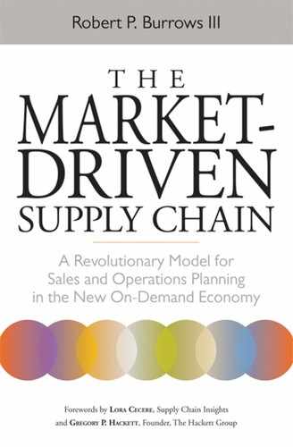
The primary tool of a zero-zero inventory strategy is the demand-sensing and balancing chart, as shown in Figure 6-2. A reference or typical historical pattern is used to predict the cumulative demand curve, as indicated in the chart by the dotted line. Actual demand is then plotted at significant points. Typically, when the season or promotion is about 25 percent booked, per the reference pattern, a comparison is made, and the total season or promotion quantity is adjusted.

Figure 6-2. EXPECTED CUMULATIVE DEMAND PLOTTED OVER THE SEASON.

Actual demand is plotted against the historical expectation or demand plan.

As an example, in the chart, the 25 percent experience has been about halfway into Period 3. We are anticipating the demand at that time to be 2,980. If we have actual demand of 3,500, we should adjust the total season or total promotion quantity up by 3,500/2,980 = 17.5 percent. The production schedule would be increased by an amount equal to the 17.5 percent increase, such that inventory would be zero at the end of the final period.

The zero-zero strategy gets its name from the common use of this tool. At the 25 percent point, you would plan to have no more than 40 to 50 percent of the total production fully committed. The first zero adjustment in production would be to calculate the production required to zero out the inventory at the end of the last period, using the newly adjusted cumulative demand plan. However, at the 25 percent point, you would authorize to produce up to only 75 to 80 percent of the total. You would leave about 20 percent of production uncommitted until the second zero point, which would be at the last possible time period for making the production commitment without causing excess costs or risking stockouts. If the production department requires one to two periods for normal lead time, the second zero should be done during Period 4 in this example. If the production managers are committing raw material to rates, the rate of production is adjusted, and lead times often are not a factor. The capacity is reserved in a RBP process, and items with long lead times are planned out of the situation.

There are, of course, some products that have such short selling seasons as to make this process unworkable, for example, Christmas tree lights. We recommend that manufacturing lead time be cut drastically with a final assembly postponement strategy or a strategy of making the final production in a somewhat-higher-cost facility with flexible, short lead-time capability. For example, laptop computers assembled in China have six- to eight-week lead times for transit. If the last piece of the production is made in the United States, the lead time for transit and assembly is about three days. In that case, the components could be used to support off-season sales, so the component inventory risk is low. The much bigger factor is the risk of making the wrong configuration of the laptops. Configuring the final 20 percent of production to demand in the United States can reduce inventory risk considerably.

So, you can keep production running smoothly over long periods of time and make schedule adjustments to the rates only twice per season. The mix of items within the family would be adjusted to demand, with a ‘C’-item scheduling strategy employed.

I have used this technique with all sorts of consumer products, hardlines products, food production, industrial pumps, and many other industries. It is close to magical. The major benefit is a drastic reduction in expediting, production changes, and excess inventory—all factors that increase free cash flow.

Capacity Definition

In all our scheduling strategies, the one underlying requirement is an agreed capacity or daily rate. The rate you want is the demonstrated rate, not a theoretical rate. A fun exercise for the design team would be to ask four different functional areas what they think capacity is and then do an analysis of actual throughput.

We did this at a food production facility with nice, clean, stainless steel production lines. I asked the master scheduler what he used for a daily rate in his production planning, and I asked him to show me the calculation; he said he used 20,000 pounds per day as the three-shift capacity. I asked the design engineer what the line was capable of producing in practical terms; his answer was 25,000 pounds. I asked the plant manager what he felt the production line team should be held accountable for; his answer was 18,000 pounds per day. I asked the foreman what he thought was a reasonable daily rate; his answer was 15,000 pounds per three-shift day. The actual throughput was 12,000 pounds per normal three-shift day.

We agreed to study why we were losing over half the design capacity. We found we had unplanned downtime of more than 20 percent, rejects for quality of 8 percent, and poor work practices that kept the line below full speed at the beginning and end of each shift and during breaks and lunch periods. The 20 percent unplanned downtime was nearly impossible to measure except in aggregate. The major factors were material jams, missed production steps, and equipment stoppages. To solve the problem, a Lean team was assigned to come up with ways to eliminate the unplanned downtime, and an unplanned downtime metric was added to the daily assessment meeting. The work practices were changed. Tag teams were used to make sure the line kept running at full production. A good deal of resistance was encountered at the beginning. The S&OP design team worked through the resistance by doing some education and by using analytics to help the production staff see and solve the problems.

The tools used in RBP are shown in Figure 6-3. The whole idea is to plan the next level of detail only when you must and not before. There is no need to worry about SKU-level detail in planning until the family is scheduled to run the next day. This is a major time savings when compared to an MRP schema. The reason the planning strategy works is because the members of the 3M family all have commonality of materials or consist of materials that can be planned to the cycle plan within the plan horizon. The differences between members of the family can be handled with minor changes in dies, stocking a few different raw materials, or using different packaging or pack sizing.

Cycle Planning

Cycle planning is an advanced master scheduling or capacity planning tool that has been around for many decades, but it was never built into the ERP systems. We know why. ERP systems were designed for the true job shop.

Cycle planning is the manufacturing manager's friend. With cycle planning, the decisions in S&OP are directly translated into manufacturing schedules. Cycle plans, unlike any other scheduling techniques, maximize flexibility in production while maintaining manufacturing economics.

FIGURE 6-3. THE FOUR PRIMARY TOOLS IN RBP.

This is a hierarchical ordering of planning activity.

In cycle planning, you calculate the maximum number of batches of the ‘A’ families you can make within the economics of setup time, a non-value-added function in total capacity. You should continue to add setups, making each ‘A’ family more frequently, until the annual line availability is used. The goal is to make the ‘A’ families multiple times per week, if possible. You leave 20 percent of the production line availability to the ‘C’ families.

From S&OP, or AOP to begin the year, the annual production quantities of each family are planned. In cycle planning, you take that information and calculate the number of batches you can make of each family. In fact, you normally set the S&OP output to have a specific number of shifts or batches for each family planned directly from the S&OP dashboard (as shown in Figure 3-1). The number is then held in the cycle-plan tool and reduced as the planner actually includes a family into the cycle plan.

A cycle plan would then look like the diagram in Figure 6-4. I normally like to see the capacity division as shifts per day. It is useful to have the line management for a shift held responsible for producing the planned quantity of each family in an easily accountable form. When responsibility for performance to schedule is limited to one management team and can be measured immediately during and after the shift, clear communication of capacity utilization can be achieved. The cycle planner needs to know if a shortfall or overproduction event has occurred so he or she can adjust the next cycle plan and definition of capacity, if necessary.

The cycle-plan diagram is self-explanatory. Each division of time—normally a shift—is set, and the family number is shown in the slot. The actual planned number of units of the family is also shown. All the planned downtime is shown in the cycle plan, including maintenance and line changes or sanitations for food production. We suggest doing cycle-plan updates once or twice a week. The plan is a rolling set of days and shifts. So for a plant with a horizon of three days, the planning can be done on Monday for Friday through Tuesday, on Thursday for Wednesday through the following Friday, and so on.

FIGURE 6-4. CYCLE PLANS DISPLAY ALL PLANNED LINE ACTIVITY.

The cycle-plan horizon is the minimum time necessary for acquisition of materials not to be taken from raw stocks.

An exception report comes out of cycle planning. The planner is given a list of families that have low or high aggregate inventory.

The basic requirement to make the cycle plan a practical solution is to plan the raw materials in a fully collaborative fashion. The objective is to have all raw materials received on or just before the shift during which they are to be used. That is planned by the supplier directly from your cycle plan.

At Anchor Foods, we had a cheese supplier that produced fresh cheese for jalapeño poppers using about 70 percent of its total capacity. Anchor seemed to always have three or four days of cheese on hand in a refrigerated holding warehouse. The maximum shelf life was right at four days, so the limits were always pushed. Sometimes, a lot went past date code and had to be trashed—an expensive occurrence. The supplier talked about the ability to supply on demand. Basically, it could produce white cheese easily to the demand. The problem was with yellow cheese. When the supplier ran yellow cheese, the equipment had to be cleaned thoroughly before it could start up on white again—a cleanup that used an entire shift, which was very expensive. We collaborated on the cycle plan and were able to schedule the yellow cheese families in such a way as to have them all produced on consecutive shifts and then switch to white. By sharing the cycle plan every few days, the supplier was able to plan to have cheese delivered at the beginning and the middle of each shift, on demand. The inventory went down to less than one shift, and the refrigeration requirements dropped to near zero.

There are four kinds of raw materials to be planned. All except type (4), which is discussed below, can be planned to the cycle plan directly. Briefly, most materials should be ordered to the actual cycle plan date and shift. We call these type (1), which are planned to the rate. Some materials are low enough in cost and space requirements to carry in stock. We call these type (2), stocked materials. Some materials can be manufactured on demand. We call these type (3), to requirements. Packaging suppliers normally are type (3). These suppliers need to plan their own production to your cycle plan and very likely have some inventory. Finally, some suppliers need to be scheduled over a longer lead time than the cycle-plan horizon. We call these type (4), long lead-time items.

Significant work is required to move all items possible to delivery on demand within the cycle plan's planning horizon. Those are the type (1) and (3) items. Basically, you can receive these materials per the cycle plan. The suppliers should have ready access to your cycle plan and should be able to plan their production in close collaboration with your cycle plan. You set up real-time, online applications in SEQUEL software to communicate with the suppliers (but do it manually first to prove the design).

If you find some type (4) items, try hard to eliminate them by moving them to type (1), (2), or (3). If you cannot, consider changing the design or dropping the product. In no case should you have more than 5 percent of the raw materials in any family in a type (4) situation. The ‘A’ families should have no type (4) items. You simply must find a way to collaborate with the suppliers for the materials going into an ‘A’ family.

The managers who do RBP well have almost all their suppliers located within walking distance, or at most, within a few hours of the point of use. Procurement needs to be encouraged to complete a full analysis of the cost versus the benefit of having suppliers nearby. In many cases, we have found suppliers’ manufacturing processes to be very flexible and/or nearly dedicated. Do not assume the lowest-cost situation is to buy from a foreign supplier. Be sure to count the transportation cost and the inventory holding costs of both finished goods and raw materials in the analysis. Use a 30 percent per year inventory carrying cost. I know accountants want to use the borrowing rate as the cost of capital, and thus, inventory carrying cost, but that is wrong. Go to the Internet and research the studies done by experts such as those at the Ohio State University to learn about inventory carrying costs; 30 percent annually is actually on the low side. Inventory is way more expensive than direct labor. In the actual Toyota Production System, having suppliers near the plant is a requirement. One of the major reasons the Japanese auto manufacturers have dramatically lower costs and inventory than the U.S. manufacturers is precisely because the supply location is very close to the use plant. Ford and General Motors run the socks off the parts before they even come close to being used.

Inventory Standards

When you must use some inventory to maintain high-capacity utilization or to manage shipping lead times to a regional warehouse, the RBP process employs an inventory standard. If you are able to produce to customer requirements within the customer's desired replenishment window, then actual orders should be used instead of the inventory standard.

Inventory standards are calculated best using an inventory simulation model. Simulation develops a reasonably accurate expected demand pattern out into the future using what is called in Operations Research (OR), a Monte Carlo simulation technique. The technique is commonly taught in operations research programs at major universities and in many MBA programs. I learned about simulation as an undergraduate at Iowa State University in the 1960s.

Why Simulation?

Simulation is a “what-if” technique, not a simple linear plot. Demand is nonlinear. In fact, our studies find well over 90 percent of the items in product portfolios have demand patterns that do not follow a normal distribution at all. Many items are random in demand or have a statistical pattern like Poisson, beta, or another of the many different types of distributions describing more randomly distributed demand patterns. Simulation allows you to study the effects of the random demand and not be fooled by the assumption of an average or normal demand pattern.

A senior executive who was a client of mine challenged me to provide an answer to a question that had perplexed him for his entire career (a long career at that). He asked, “Can you tell me why I have a very large inventory and still have stockouts on many items?” The answer I gave was by way of an example. In standard supply chain software—his company was using one of the most popular brands—safety stock is estimated using average demand and the three-sigma limit of the variation in demand. The software did not automatically check to see if the statistical calculation of a three-sigma limit had any relevance or fit inside a reasonable range of err. If the software had done the checks for relevance and calculated the err range, the company would have found the calculation did not provide much protection against a service failure. Consider an item with a demand pattern per week of the following: 3-0-0-0-0-0-5-0-0-0-0-0-0-0-3-0-0-0-5-0-0-0-0-0-0-3, etc. The average over the six months shown, 26 weeks, is .73 per week. The three-sigma limit would be 2.5. So the system would carry about three or four in stock. For 21 of the 26 weeks, the safety stock would be considered excess inventory. But for each week in which there is demand of five, the safety stock does not satisfy the demand, and there is a service failure. It could be that one customer has a rule to order in lots of five and another in lots of three. These are not average or normal; they are arbitrary. Thus, you carry excess inventory and still have stockouts. When I finished giving the executive this explanation, he hired us on the spot; he was overjoyed at finally having an answer to his question. Simulation would have suggested a stocking level of five and replenishment to five after each week in which demand was determined. If lead time was longer than a week, I believe the system would most likely have ignored that fact; the users probably don't understand the requirement for safety stock to be variation in demand over lead tine. This is not the users’ fault but is a software training deficiency.

Another common technique for calculating what system inventory should be is so-called optimization. The technical term is linear programming (LP). The word optimization is used as a marketing term. Who would object to having their inventory optimized? The problem with linear programming, though, is that solving for “optimum” inventory in a random demand world is not linear. Linear programming was used before we had nearly free memory in laptops and massive amounts of computing power. The laptops today are many times more powerful than the computers in computer rooms in the 1970s and the first laptops in the 1980s. Since LPs are simple and reasonably small, the old computers could handle them with ease. The programs provided useful information, given the limits of computing power 30 years ago. A small simulation problem would have overwhelmed the computers of the 1970s and 1980s, when most supply chain software was developed. Today, it is not unusual to have a laptop with sufficient memory and computing power to solve even complex simulation models. We had an automotive client with 180,000 items stocked in more than 30 locations. We ran a simulation model to solve for the inventory requirements in a matter of a few hours. All the “what-if” scenarios were completed in a few days. The emphasis is on analysis, not crunching numbers.

Inventory Standards Replace Safety Stock

Inventory standards represent the inventory level that results from the cycle plan's expected frequency of production versus the Monte Carlo—simulated future demand by SKU. The inventory standard is set based upon the desire to avoid stocking out. If you wish to have no chance of a stockout, set the standard at double the level the simulation calculates as safe. If you want reasonable inventory levels, use the basic inventory level the simulation calculates.

The simulation runs through “what-if” scenarios to calculate the resulting inventory. As production frequency increases or initial inventory is increased, the occurrences of a projected shortage are reduced. The cycle plan restricts the number of batches of a family to be allowed over the planning horizon, say, a season or more than six months. So the inventory level will be increased and then float from a very low level to a higher level. The inventory standard is usually chosen to be such that at 50 percent of the standard, a projected shortage never happens or is so infrequent as to be irrelevant. The inventory standard then sets the mean with 50 percent being the lower control limit and 150 percent being the upper control limit.

Inventory standards function as a barometer of inventory, not as a safety stock. The actual production is to demand when the cycle plan has a family scheduled to be produced. The inventory standard never triggers production by itself. Production is always planned with the cycle planner, and inventory deployed is by SKU through rate mix.

Rate-Mix Planning

Rate-mix planning is done the day before production, per the cycle plan for each family. The planning tool schedules the quantity required by the cycle plan. The individual SKUs, if produced to plan, have the same stocking level as compared to their individual inventory standards. That is, they should have the same exposure to a stockout and the same probability of having the actual demand satisfied with minimal inventory.

The form shown in Figure 6-5 is a snapshot from a rate-mix planner programmed into a homegrown planning system by one of our clients. We developed the logic and detail in Excel first and then let the IT staff go to work once the process was fully vetted.

The figure shows a simple example of a production line that is making four different families of product that day with specific products in each family. In the example, family 211, with product number 983, is scheduled for production. The product is stocked in three different locations, or has three SKUs. The planner determines how much to send to each of the three locations. Note the information displayed:

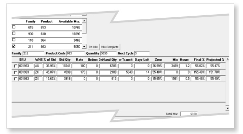
FIGURE 6-5. THE RATE-MIX PLANNING TOOL.

The rate-mix tool balances SKU inventory. It can be set up in a database or in Microsoft® Excel with minimal effort.

The percent of the inventory standard on hand now.

The most recent calculation of daily rate of consumer take-away.

The on-hand quantity.

The in-transit quantity from the last batch of production or another source, such as released from quality hold.

The days remaining on hand or in transit now.

The percent of inventory standard that would be remaining if you produced zero.

The calculated mix the computer is determining: a total of 5,050 units, with 1,561 going to one SKU and the remainder to another. (None is going to the third SKU.)

The two SKUs produced will be balanced at about 55 percent of the standard. The middle SKU will have an excess as a result of the in-transit quantity.

The final percent is the inventory balance after the production day.

The projected percent is the expected inventory level at the next scheduled batch of this family, which is in five days per the header information.

The rate-mix planner runs in minutes and shows the detail for each item being produced tomorrow. Once the planners are comfortable with the process, very little intervention is necessary, and detailed production orders can be written. In most cases, the planning output becomes input to whatever existing transaction software is being used to generate the electronic instructions for the production lines.

You will have an exception report coming out of rate mix, similar to the one from cycle plan. If the percent to standard is below, say, 50 percent, after the production plan is set, the planner is notified to consider moving the family up in the cycle-planning process. If the family's inventory is more than 150 percent of the standard, the next cycle plan may see the family moved out.

Why It Works

Rate-mix planning works because the raw materials are required only when the products into which they go are being manufactured. This is a simple fact, but one that is often overlooked. Most mangers think they need to have a decoupling of the supplier and the manufacturing line. Another term for this decoupling is an inventory. However, if the supplier can operate at the same rate as the manufacturer, only offset by a few hours or a day, then there is no need to decouple and create an inventory. The major raw materials for most products can be arranged to operate at a collaborative rate rather than be built to inventory. This is true even if the lead time between the supplier and the manufacturer is very long—for example, if you are buying a large component from a source in Hungary, which is three weeks away by boat from the assembly plant in the United States. If the assembly plant works to a cycle plan, then the supplier can predict the timing and delivery day required for each component with a high degree of accuracy.

We had a client that made a complex capital equipment item for banks. The company sourced one major component in Eastern Europe and another in China. Lead times were long. The practice was to use MRP and safety stocks, ignoring the idea of using a cycle plan and building to rates. Raw materials inventory was large, because the company calculated safety stock in the standard MRP method of variation in demand over lead time. The company assumed lead time at its worst, 22 weeks, which was the time from the Eastern European supplier's start of procurement of materials to the time of delivery to the U.S. factory. If the client had used the rate-based method and rate-mix planner with a cycle plan, it would have been able to carry only the in-transit inventory that it did not own, or zero inventory on the balance sheet. There is no variation in demand in cases such as this, because the raw material is used only when production is scheduled. The client also carried a great deal of finished goods inventory, so it had truly no need for safety stock in raw material. Thus, a major inventory reduction opportunity was found.

This process is designed to let inventory for items within a family actually float inside a control limit, so the production plan for the next few months is not constantly being disrupted.

The possibilities for extension of the rate-mix process into logistics management are significant. We have used the SKU detail, which is by stocking location, to plan warehouse operations. You can run a planning report from the rate-mix detail that tells you how many truckloads or less-than-truckloads (LTL) of product will be loaded for shipment. The warehouse employees can spot trucks into loading bays and then let them sail when they are full or hold them until the LTL load is finished for the day. Packaging lines managers can be told how many boxes, labels, and the like should be staged ahead of production the next day. Quality control can make its plans for sampling and so on.

Major Benefits

RBP and rate-mix planning specifically can provide a significant reduction in the planners’ daily workload. Take, for instance, a company with 1,500 product items stocked in eight warehouses, with both company and customer VMI locations. In an MRP world, the planner deals with the total number of SKUs all the time, or with more than 12,000 SKUs. On any given day, the demand for many of the SKUs is different from the normal distribution assumptions used automatically in the computer software. A planner will be given exception reports with perhaps hundreds or thousands of line items. In practice, the exception reports are ignored because of their sheer volume, and they are just passed on to production, where changes in production schedules are very frequent. In one client of ours with approximately this level of SKUs, the production scheduling staff held meetings with production twice daily to discuss major schedule changes of eight to ten different production orders each time. The client also had high variability in production orders not yet released. The result was much chaos and confusion. In the rate-based world, the planner handles two or three families of items each day and nothing more. The level of schedule changes is almost irrelevant, and the planner can focus on improvements and refinements, rather than the non-value-added functions of expediting and handling objections from foremen and suppliers who are being disturbed with schedule changes.

In the rate-based world, suppliers are truly collaborative partners. The suppliers see a much more stable production requirement than is found in the MRP chaos. Suppliers often discover they can reduce changeover costs, eliminate costly inventory, and find available capacity. They will then be open to reducing prices.

Looking Back

These are the principles of rate-based planning (RBP):

Build to an order rate, not to an order.

Don't make a decision until you have to.

RBP applies to almost all manufacturing types.

RBP replaces MRP and JIT, which do not respect capacity limitations and work independently of S&OP.

MRP and JIT require excessive capital expenditures and excess inventory investment. Both methods are counterproductive to good business management.

The scheduling strategies in RBP reduce the peaks and valleys of demand variation by using ‘A’ items or order backlog as buffers.

A zero-zero strategy reduces inventory overhang in seasonal and promotional businesses.

Cycle plans flow directly from S&OP and maximize production flexibility without violation of manufacturing economics.

Inventory standards are a barometer of demand, recognizing changes in demand rates to expectations, while maintaining production line schedule stability.

RBP generates the SKU-level inventory flow by managing to demand—ideally “at market” demand, not some intermediate surrogate.

The benefits of the RBP approach are better utilization (more throughput), less time spent doing non-value-added clerical functions like expediting, and lower raw material costs.
 

RBP delights customers, provides cash for investment, and enables employee job enrichment—a win-win-win situation.