
Chapter 2. Bridges and Tools for Learning Graph Thinking
Together over the years, we have advised hundreds of teams on what, where, and how to get started with graph data and graph technologies. From those conversations, we collected the most common questions, difficulties, and advice for introducing graph thinking and graph data into your business.
We want to start your journey towards graph thinking with the following three questions that every team will encounter when evaluating graph technologies:
-
Is graph technology better for my problem than relational?
-
How do I think about my data as a graph?
-
How much do I need to learn in order to get started with graph technology?
Those teams which spend the time upfront understanding these three topics are more likely to successfully integrate graph technologies into their stack. Conversely, from our experience, businesses shelved early stage graph projects because their teams skipped through collectively understanding these questions for their business.
Ultimately, the introduction of graph data into your application brings a new paradigm of thinking about what is important within your data.
Graphs emphasize relationship first design instead of entity first design.
Understanding the differences in these principles starts with evolving your mindset from relational to graph thinking.
Let’s preview what this chapter will cover to get you started on your own journey with graph thinking.
TL;DR Translating relational concepts to graph terminology
Throughout the rest of this chapter, we will walk you through the process and details for each of the three questions at the beginning of this chapter. We will start off with an abbreviated tour of the differences in relational andcreating a conceptual database model for a relational system. From the model, we will translate the relational concepts to graph modeling techniques. We will introduce and use the Graph Schema Language (GSL) to build up a conceptual graph model. We will conclude this chapter with a short tour of some fundamental terms from graph theory.
Inevitably, you are going to have to make some tough decisions about if, where, and how to introduce graph thinking and technology into your workflow. In this chapter, we are going to introduce tools and techniques to help you navigate a large pool of technical opinions. The foundations we introduce will help you evaluate if graph technology is the right choice for your next application.
The concepts and technology decisions introduced in this chapter will serve as the foundational material for our future examples. We are using this chapter to clearly illustrate the vocabulary that we will use to describe graph database schema and graph data in the examples throughout this book.
Relational Versus Graph: What’s the Difference?
So far, we have mentioned two different technologies: relational and graph. When we talk about relational systems, we are referring to organizing your data in a way that focuses on the storage and retrieval of real-world entities, eg: people, places, and things. When we talk about graph systems, we are referring to systems which focus on the storage and retrieval of relationships. These relationships represent the connection between real-world entities: people know people, people live in places, people own things, etc.
The line between when to select a relational or graph system for your application is grey; there are benefits and drawbacks for each choice. Choosing between a relational or graph database typically generates a conversation between storage requirements, scalability, query speed, ease of use, and maintainability. While any aspect of this conversation is worth discussing, we aim to shed more light on the more subjective criteria: ease of use and maintainability.
Note
Relational versus Relationships: even though these two words are very similar, we use them explicitly in reference to two different types technologies. The word relational describes a type of database, like Oracle, MySQL, PostgreSQL, IBM DB2, … etc. These systems were created to apply a specific field of mathematics to data organization and reasoning, namely relational algebra. On the other hand, we use the word relationship solely in reference to graph data and graph technologies. These systems were created to apply a different field of mathematics to data organization and reasoning, namely graph theory.
Choosing between relational and graph technologies can be difficult because you are cannot compare them at a feature-functionality level. Their differences run to the core of being built based on distinct mathematical theories: relational algebra for relational systems and graph theory for graph systems. That means the suitability of each technology depends to a large degree on the applicability of those theories and their associated line of thinking to your problem.
We are going to drill into the differences between relational and graph technologies a little further in the following sections for two reasons. First, since most people are familiar with relational thinking, we can introduce graph thinking in contrast to relational thinking. Second, we want to provide a response to the inevitable question of “why not just use an RDBMS?”. Both of these reasons are important to explore in the context of understanding graph technology because relational systems are very mature and widely adopted.
Throughout this entire book, we will use data to illustrate concepts, examples, and new terminology. Let’s start with the data that we will be starting with in this chapter to illustrate the differences between relational and graph concepts. You will see this data in the example that spans Chapter 3, Chapter 4, and Chapter 5.
Data for Our Running Example
We will use the data in Table Table 2-1 to construct relational and graph data models.
For our first use case, the data describes a customer’s assets in the financial services industry. The customers can share accounts and loans, but a credit card can only be used by one customer.
Let’s look at a few rows of the data. Table 2-1 displays data about five customers. These five customers and their data will be used to build data models and illustrate new concepts throughout the next four chapters.
| customer_id | name | acct_id | loan_id | cc_num |
|---|---|---|---|---|
customer_0 |
Michael |
acct_14 |
loan_32 |
cc_17 |
customer_1 |
Olivia |
acct_14 |
none |
none |
customer_2 |
John |
acct_5 |
none |
cc_32 |
customer_3 |
David |
acct_0 |
loan_18 |
none |
customer_4 |
Emma |
acct_0 |
[loan_18, loan_80] |
none |
There are five unique customers in the five rows of sample data shown in Table 2-1. Some of these customers share accounts or loans to illustrate different types of users we typically see in a financial services system.
For example, customer_0 and customer1, namely Michael and Olivia, represents a typical parent-child relationship; Michael is the parent and Olivia is the child. The data about customer2, John, indicates he or she is a sole user of this financial service. We usually see the highest volume of this type of user in large applications. Customers like John only have data that is unique to the customer and is not shared by anyone else. Lastly, customer3 and customer4, David and Emma, share an account and a loan. This type of data typically indicates these users are partners who have joined their financial accounts.
If this were your company’s sample data, imagine the conversation you would have about modeling this data with your coworker. In this scenario, you are sharing a white board, or other illustrative tool, and you are trying to map out the entities, attributes, and relationships within the data. Whether or not you use a relational or graph system, you likely would be having a discussion similar to the conceptual model in Figure 2-1.

Figure 2-1. A conceptual description of the relationships observed in the data in Table 2-1.
From Table 2-1, we find four main entities: customers, accounts, loans, and credit cards. These entities each have relationships tied to the customer. Customers can have multiple accounts and those accounts can have more than one customer. Customers can also have multiple loans and those loans can have more than one customer. Lastly, customers can have multiple credit cards, but that credit card is unique to the customer.
Relational Data Modeling
Your transition from relational and into graph thinking starts with data modeling. Understanding data modeling in these two systems begins to illustrate why graph technologies can be a better fit.
For anyone who has been a database practitioner, you’ve probably been introduced to visual ways of modeling data in a relational system. The most popular choices for creating relational data models are to use the unified modeling language (UML) or entity-relationship diagrams (ERDs).
In this section, we will use the example data from Table 2-1 to complete an abbreviated walk through of a relational data modeling with an ERD. We have included just enough information in this section to be a first step from relational to graph thinking. This is not intended to be used as a full introduction into the world of relational data modeling. We recommend the seasoned book by C. Batini et al. for a complete detail on relational data modeling. And, for those of you who are very comfortable with third normal form, you can skip this next bit and head directly “The Graph Schema Language”. 1
Entities and Attributes
Generally speaking, data modeling techniques help you describe the real world by describing the entities and their attributes within your data. Each of those concepts has a specific meaning:
-
An entity is an object such as a person, place, or thing that you need to track in your database.
-
An attribute refers to a property about an entity like names, dates, or other descriptive features.
The traditional approach for relational data modeling starts with identifying the entities (people, places, and things) in your data and the attributes (names, identifiers, and descriptions) about the entities. Entities could be customers, bank accounts, or products. Attributes are concepts like a person’s name or bank account number.
For this exercise in data modeling, let’s start by modeling two entities from Table 2-1.: customers and bank accounts. In a relational system, we traditionally view the entities as tables. This is illustrated below in Figure 2-2.

Figure 2-2. The traditional approach to modeling the data within your application: identifying the entities and their attributes.
There are two main concepts shown in Figure 2-2: entities and their respective attributes. There are two entities in this diagram: customers and accounts. For each entity, there is a list of attributes that describe the entity. A customer can be described by a unique identifier, name, birth date, etc. There are also descriptive attributes for accounts: a unique account identifier and the date the account was created.
In a relational database, each entity becomes a table. The rows of the table contain instance data of that entity and each column contains values for the descriptive attributes.
Building up to an ERD
In the real world, customers own accounts. The next step in designing a relational database would be to conceptually model this connection. We need to add to our model a way to describe how a person owns a bank account. A popular method for modeling the link from customers to accounts is shown in Figure 2-3.
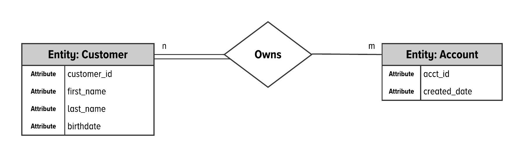
Figure 2-3. An entity-relationship diagram for customers and bank accounts.
We added one visual element between Figure 2-2 and Figure 2-3. This is shown as the diamond that connects the person and account entity tables. This indicates that there is a link between customers and accounts in the database. Namely, customers own accounts.
The other visual details in the image are shown with the double lines between the person table and the owns connection. Here, we see an n, with an m on the opposite side. This notation indicates that this is a many-to-many connection between customers and accounts. Specifically, this translates to that one person can own many accounts and that one account can be owned by many customers.
The following nuance about the implementation details is important: links that are shown in ERDs translate to tables or foreign keys. That is, the connection between customers and their account is stored as a table within a relational system. This means that the owns table essentially translates to another entity in the database.
Note
Using tables to represent the connections within your data as entities makes it more difficult to understand the links within your data. The mental leap from natural understanding to tabular retrieval is a significant mental hurdle to overcome. This is especially true when you need to understand the connectedness of your data.
Even though we have been forced to think this way for decades, there are better ways.
Let’s revisit the same data from Table 2-1. However, this time, we are going to use the data to illustrate concepts in graph data followed by how we will model the data in a graph database.
Concepts in Graph Data
We will use this section to introduce useful terminology from the graph theory community. These terms are used to describe the connectivity of the graph data. Let’s visualize the graph data about the first three people from our sample data.
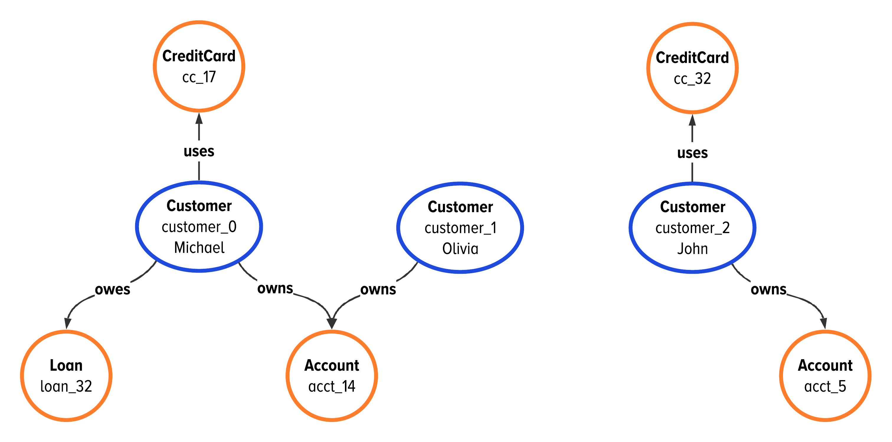
Figure 2-4. A look at the graph data we will use to introduce new graph terminology in this chapter.
The data illustrated in Figure 2-4 will be used to illustrate the fundamental concepts in the rest of this section. This data contains information about three people: Michael, Olivia, and John. Michael and Olivia share an account, as seen in Figure 2-4. John does not share any data in common with the other two customers in our example.
Fundamental Elements of a Graph
The first concepts we need to introduce are the fundamental elements of graph, graph data, and their definitions. These terms are used across all members of the graph community and are accepted as the fundamental elements of a graph.
-
A graph is a representation of data with two distinct elements: vertices, which are also called nodes, and edges, which are relationships or links from one vertex to another.
You have already seen the fundamental elements we are talking about. Our financial data from Figure 2-4 contains four conceptual entities: customers, accounts, credit cards, and loans. These entities naturally translate into the vertices of our graph.
Next, we use edges to connect our vertices. These connections illustrate the relationships that exist between the pieces of data. In graph data, an edge connects two vertices as an abstract representation of a relationship between the two objects.
For this data, we will use edges to show the relationship between a person and their financial data. We model the data to say that the customer owns accounts, the customer owes loans, and the customer uses credit cards. The edges in the graph database become the relationships of owns, owes, and uses.
Together, all of the vertices and edges in the data represent the full graph.
Adjacency
While there are many foundational topics in graph theory to explore, the term to start with is adjacency. You will find this term throughout graph theory to talk about how data is connected together. Essentially, adjacency is the mathematical term used to describe if vertices are connected together. Formally, it is defined as follows.
-
Two vertices are adjacent if they are connected by an edge.
In Figure 2-4, Olivia is adjacent to acct_14. Also, we see that both Michael and Olivia are adjacent to acct_14 because they both own that account. The benefit to using graph data in your application is immediately seen when you can find how different entities are related in a way that you may not have previously seen.
The idea of adjacency will come up many more times throughout this book in topics ranging from the connectedness of data to different storage formats on disk. For now, it is only important to know that this popular term is referring to how vertices are connected.
Neighborhoods
Data that is connected forms communities. In graph theory, these communities are called neighborhoods. For a vertex, all adjacent vertices are in its neighborhood. You will see this written as: N(v). All vertices within a neighborhood are said to be neighbors.
-
For a vertex
v, all vertices that are adjacent tovare said to be within the neighborhood ofv, writtenN(v). All vertices within a neighborhood are neighbors.

Figure 2-5. A visual example of graph neighborhoods starting from customer_0.
Figure 2-5 shows the concept of graph neighborhoods starting from customer_0, Michael. In this sample data, the vertices cc_17, loan_32, and acct_14 are directly connected to, or adjacent, to Michael. We call this the first neighborhood of customer_0.
You can continue this concept by walking further away from the starting vertex. The second neighborhood are those vertices that are two edges away from Michael; Olivia is in the second neighborhood of Michael. It also works to say the reverse, that Michael is in the second neighborhood of Olivia. This can continue on throughout the graph as we walk through the full depth of vertices from a singular starting point.
Distance
The concept of neighborhoods brings us to distance. Another way to talk about the connectedness of this sample data is to say how many steps it takes to walk from one vertex to another. Talking about Micheal’s first or second neighborhood is the same as finding all vertices that are a distance of one or two from Michael.
-
In graph data, distance refers to the number of edges that you have to walk through to get from one vertex to another
In Figure 2-5, we selected the starting point as the vertex Michael. The vertices cc_17, loan_32, and acct_14 are in Michael’s first neighborhood, which is the same as a distance of one away from Michael.
In mathematical communities, you will see this written as dist(micheal, cc_17) = 1. That also means that everything in the second neighborhood from your starting point is two edges away, etc. Specifically, dist(Michael, Olivia) = 2.
Degree
The ideas of adjacency, neighborhoods, and distance help us understand if two pieces of data are connected. For many applications, it is really useful to understand how well a piece of data is connected to its neighbors.
The difference between if versus how well data is connected introduces a new term from the math community: degree.
-
A vertex’s degree is its total number of edges that connect it to other vertices in the graph.
-
A vertex’s in degree is its total number of incoming edges that connect it to other vertices in the graph.
-
A vertex’s out degree is its total number of outgoing edges that connect it to other vertices in the graph.
To apply this, refer back to Figure 2-4. Here, we see that there are three edges that connect Michael to cc_17, loan_32, and acct_14. We apply this to say that the degree of Michael is 3, or deg(Michael) = 3.
In this data, we have two vertices that have degree two. Specifically, acct_14 is adjacent to Michael and Olivia, so it has a degree of two. On the right side of the image, we also see that John has only two edges. That means that John has a degree of two.
There are a total of five vertices in our example data that have a degree of one. They are loan_32, cc_17, Olivia, cc_32, and acct_5.
Note
In graph theory, vertex with a degree of one is called a leaf.
Data scientists and graph theorists use a vertex’s degree to understand the type of connections found within their graph data. One of the first places to start is to find the most highly connected vertices within your graph. Depending on the application, vertices of very high degree can be thought of as hubs or highly influential entities.
It is useful to find these highly connected vertices because they also have performance ramifications when storing or query them in a graph database. To a graph database practitioner, vertices of extremely high degree (>100,000 edges) are known as supernodes.
For the purposes of this section, we want to being to illustrate how to apply and interpret graph structure in your application. We will get into the performance details of highly connected vertices later.
The Graph Schema Language
Graph practitioners, academics, and engineers have generally agreed on terms and methods for illustrating graph data. However, the terms are confusingly used across the technical and academic communities. There are many cases when the same word to a graph database practitioner means something different to a graph data scientist.
To address confusion across the communities, in this book we are introducing and formalizing terminology to describe graph schema. This language is called the Graph Schema Language: GSL. The GSL is made up of a visual language to apply concepts to create graph database schema.
We created the GSL as a teaching tool to use throughout the examples in this book. Our purpose in creating, introducing, and using the GSL is to normalize how graph practitioners communicate conceptual graph models, graph schema, and graph database design. To us, this set of terminology and visual illustrations is complementary to the graph languages popularized by the academic community and the standardization initiatives within the graph community.
We will use the visual cues and terminology described in this section throughout the conceptual graph models used in this book. We hope the many upcoming examples are good practice for translating a visual schematic into schema code.
Vertex Labels and Edge Labels
The fundamental elements of graph data, vertices and edges, give us the first terms of the Graph Schema Language (GSL): vertex labels and edge labels. Where relational models use tables to describe the data in Figure 2-3, we use vertex labels and edge labels to describe a graph’s schema.
-
A vertex label is a set of objects that are semantically homogeneous. That is, a vertex label represents a class of objects that share the same relationships and attributes.
-
An edge label names the type of relationship between vertex labels in your database schema.
In graph modeling, we label each entity with a vertex label and describe the relationship between entities with an edge label.
Generally speaking, vertex labels describe entities in your data that share attributes of the same type and relationships of the same label. Edge labels describe relationships between vertex labels.
Note
The terms vertices and edges are used in reference to data. To describe a database’s schema, we use the language vertex labels and edge labels.
For the data from Table 2-1, we would model the same customer and account with the conceptual graph model shown in Figure 2-6. This conceptual graph model looks very similar to the ERD from Figure 2-3, but with the translation to using the first two terms of GSL.
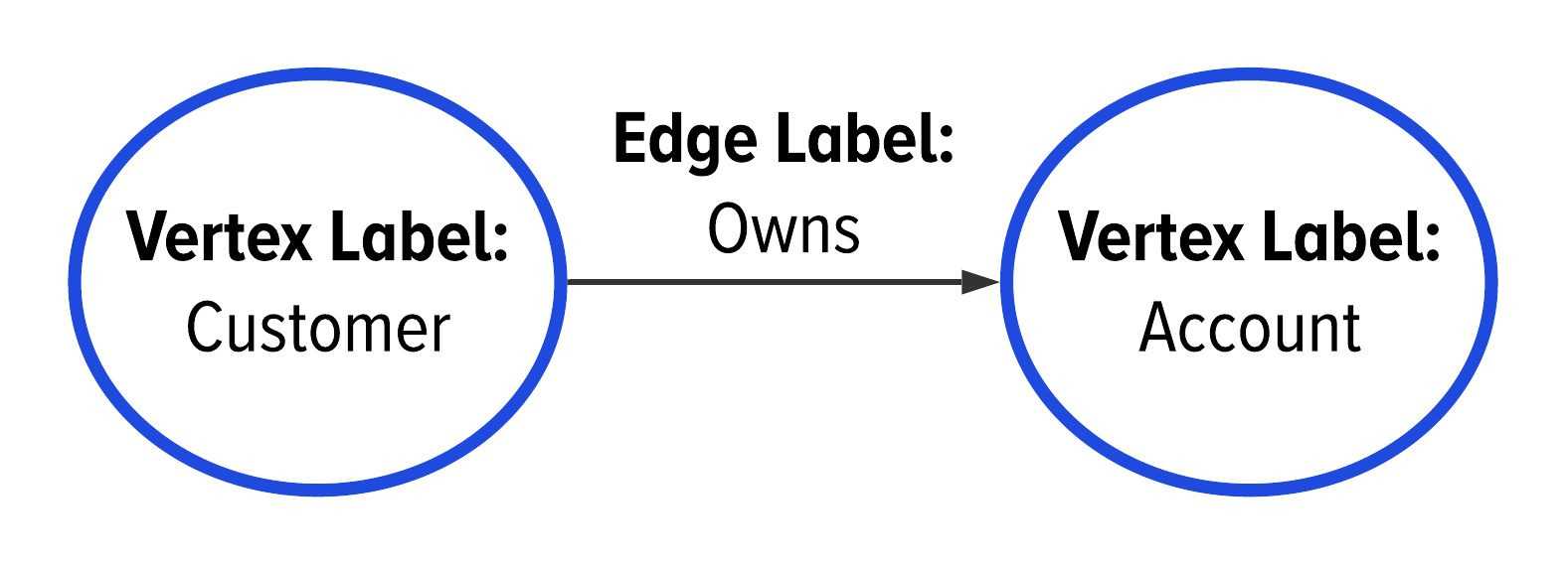
Figure 2-6. A graph model showing the vertex and edge labels for customers and bank accounts.
In the GSL, a vertex label is illustrated with a circle containing the label’s name. Figure 2-6 shows this for the Customer and Account vertex labels. An edge label is illustrated with a named line between two vertex labels. We see this in Figure 2-6 with the owns edge label between the Customer and Account vertex labels. When we look at this illustration, we infer that a customer has a relationship to an account; specifically that the customer owns the account. We will get into an edge’s direction later in “Edge Direction”.
Properties
Where relational models use attributes to describe the data in Figure 2-3, properties describe data in graph modeling. That is, where we had attributes before, we have properties in a graph model.
-
An property describes features of a vertex label or edge label, like names, dates, or other descriptive features.

Figure 2-7. A graph model for customers and bank accounts.
In Figure 2-7, each vertex label has a list of properties associated with it. These properties are the same attributes from the relational ERD in Figure 2-3. A customer vertex is described by its unique identifier, name, and birth date. An account is described with its account id and created date, as before. We add an edge label of owns to describe the relationship between the two entities in this data model.
Note
Note that the term property applies to concepts in graph schema and graph data.
Edge Direction
The next modeling concept defined in the GSL is an edge’s direction. When we set up our edge labels in our data model, we connected the vertex labels together in a way that follows how we would naturally talk about the data. We say that a customer owns an account and we modeled the data in our graph that way. This also gives each edge a direction.
There are two ways in which you can model the direction of an edge: directed and bidirectional.
-
A directed edge goes one way: from one vertex label to the other vertex label.
-
An bidirectional or bidirected edge goes both directions between the vertex labels.
Using GSL, we indicate the direction of an edge with arrows on either one or both sides of the edge line. This is illustrated in Figure 2-8 with the arrow on the edge label.
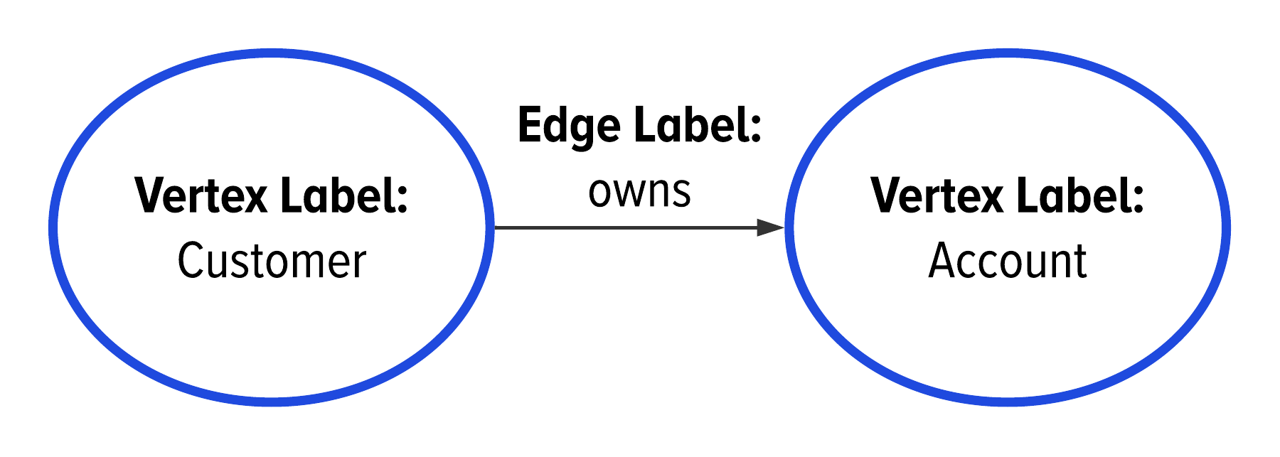
Figure 2-8. The use of a line with a singular arrow to indicate that an edge label is directed.
In our example from Figure 2-8, we would say that this shows a directed edge label. We have an edge label that goes from the customer to an account. This edge label uses a directed edge to model that a customer owns an account.
On the other hand, it might be useful to model our data in the opposite direction. One way to do this is by adding a second directed edge from the account to the customer. This edge indicates that the account is owned by the customer, like in Figure 2-9. We say that all of the edges in Figure 2-9 are directed because they only go one way.
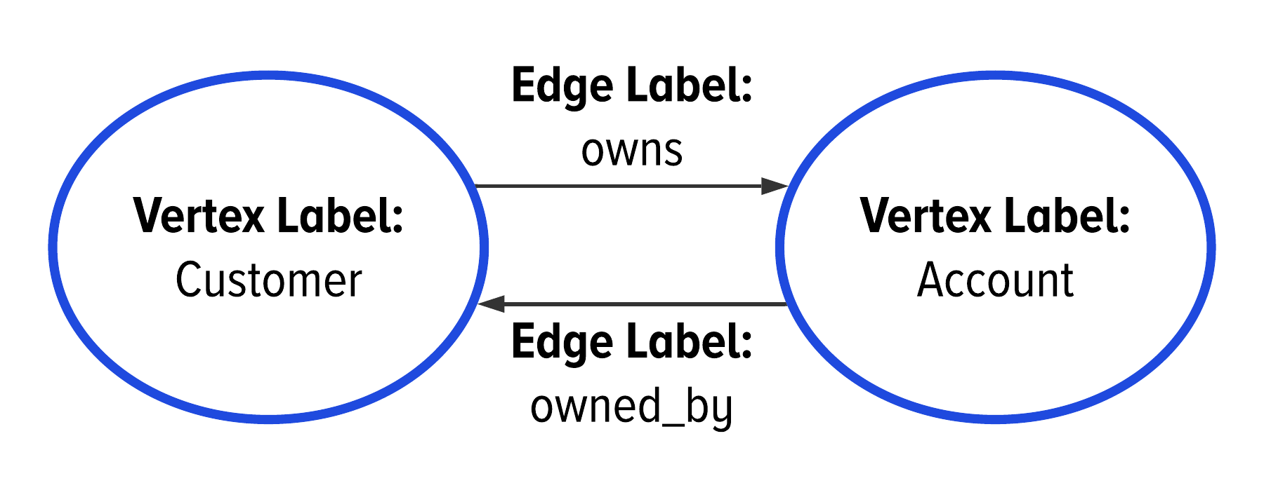
Figure 2-9. The use of a line with a singular arrow to indicate that an edge label is directed.
An edge label’s direction comes from how we communicate about our data. When you describe your data, you use a subject, predicate, and object to communicate about your domain. To see this, consider how you would describe the sample data we have been using so far in this chapter. You likely are thinking something like “bank accounts are owned by customers” or “customers own accounts”. In these phrases, the subject is “customer”, the predicate is “owns”, and the object is “accounts”. This gives us a source vertex label: “customer”, a predicate “owns”, and a destination vertex label “account”. The predicate “owns” translates to an edge label and has direction from the customer to their account.
Loosely, the identification of the subject, predicate, and object of your description creates an edge label’s direction. The subject is the first vertex label and is where an edge label starts. In the GSL, we call this the domain. Then, the predicate becomes your edge label. Lastly, the object is the destination or range of an edge label. This means the edge label comes from the range and goes to the domain. This gives us two new terms:
-
The domain of an edge label is the vertex label from which the edge label originates or starts.
-
The range of an edge label is the vertex label to which the edge label points or ends.
The last concept to illustrate in this section is a bidirectional edge. For the data we have talked about so far, it doesn’t exactly make semantic sense to have an edge label that goes in both directions. That is, it is meaningful to say that a customer owns an account but it doesn’t make sense to say “an account owns a customer”. We have to change the edge label to say that “an account is owned by a customer”.
To best illustrate an edge label that is bidirectional, let’s add relationships between customers into our example. Specifically, let’s add an edge label that connects customers who are family members. This is a better example to illustrate a bidirectional edge label and is shown below in Figure 2-10.

Figure 2-10. The use of a line with two arrows to indicate that an edge label is bidirectional.
In this model, we are indicating that customers can be family members of other customers. We interpret this type of relationship as a reciprocal relationship: if you are a family member to someone else, they are also your family member. We model this in the GSL using a line with an arrow on both ends and say that this edge label is bidirectional or bidirected.
Note
In graph theory, a bidirected edge is the same thing as an undirected edge. That is, modeling a relationship in both directions is essentially the same as not having one specific direction. However, in the context of this book, we are using relationships between data to provide meaning to an application and therefore have to consider an edge’s direction.
When first encountering direction, it can be a tricky concept to wrap your head around. In graph development, one of the best ways to think about direction comes from how you speak about your data. We recommend creating a description of your data and identifying how you would explain the relationships within it. This helps mentally translate your conceptual understanding of your data’s relationships into an edge label’s direction
Self-Referencing Edge Labels
Without explicitly calling it out, we introduced a new concept in Figure 2-10 that we would like to define now. If an edge starts and ends on the same vertex label, we say that is a self-referencing edge label. In the GSL, we would draw and notate this as seen below in Figure 2-11.
-
A self-referencing edge label is where the edge label’s domain and range are the same vertex label.
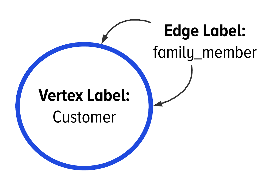
Figure 2-11. The use of an edge label in the GSL to indicate a bidirectional, self-referencing edge.
Figure 2-11 is the correct way to illustrate an edge label that starts and ends on the same vertex label. We say that this is a self-referencing edge label. In the case of Figure 2-11, this is also a bidirected edge label. However, not all self-referending edge labels are bidirected.
Note
You will see an example of a directed, self-referencing edge label in an upcoming chapter. This is the case when you need to model recursive relationships. Specifically, when something is contained within something else or if you have a parent-child relationship.
Multiplicity of your Graph
When you start diving into data modeling with graphs, you probably want a way to indicate how many relationships can exist between different vertex labels in your graph.
We have some good news on this topic. There is only one option for describing the number of relationships in most graph models: many.
In DataStax Graph, and most other graph databases, all edge labels represent many-to-many relationships. Meaning, any vertex can have many other vertices connected to it by a particular edge label. In an ERD, this is called many-to-many, in UML you use 0..* to 0..*. Sometimes, this is also referred to as an m:n relationship within the relational community.
We use multiplicity to describe this concept:
-
Multiplicity is a specification of the range of allowable sizes that a group may assume.
-
Namely, multiplicity describes the range of allowable sizes that the group of adjacent vertices to a given vertex along a particular edge label may assume. 2
Note
The actual size of the set or collection is referred to as cardinality. The definition of cardinality is: cardinality is the finite number of elements in a particular set or collection.
For correctness and clarity, we exclusively use the term multiplicity when talking about modeling edge labels within a graph schema. Let’s dig a little deeper into the two options you have when you apply the definition of multiplicity in your graph model.
Modeling Multiplicity in the GSL
The application of multiplicity to your graph’s schema comes down to understanding the differences between what kinds of groups of adjacent vertices are possible. There are only two: a set or a collection.
-
A set is an abstract data type that stores unique values.
-
A collection is an abstract data type that stores nonunique values.
In a set of adjacent vertices, there can only be one instance of a vertex. In a collection of adjacent vertices, there could be many instances of a vertex. We illustrate the difference between these concepts in Figure 2-12.

Figure 2-12. The two options for applying multiplicity to the group of adjacent vertices for a specific edge label.
The graph on the left of Figure 2-12 shows that the group of vertices adjacent to Micheal is a set: {acct_0}. This means that we want to have at most one edge between a customer and an account in our database. The graph on the right of Figure 2-12 shows that the group of vertices adjacent to Micheal is a collection: [acct_0, acct_0]. This means that we want to have many edges between a customer and an account in our database.
Let’s show how we would model the differences between the two graphs from Figure 2-12 in the GSL.
Figure 2-13 shows how we use a single line in the GSL to illustrate that we want to have at most one edge between two vertices.
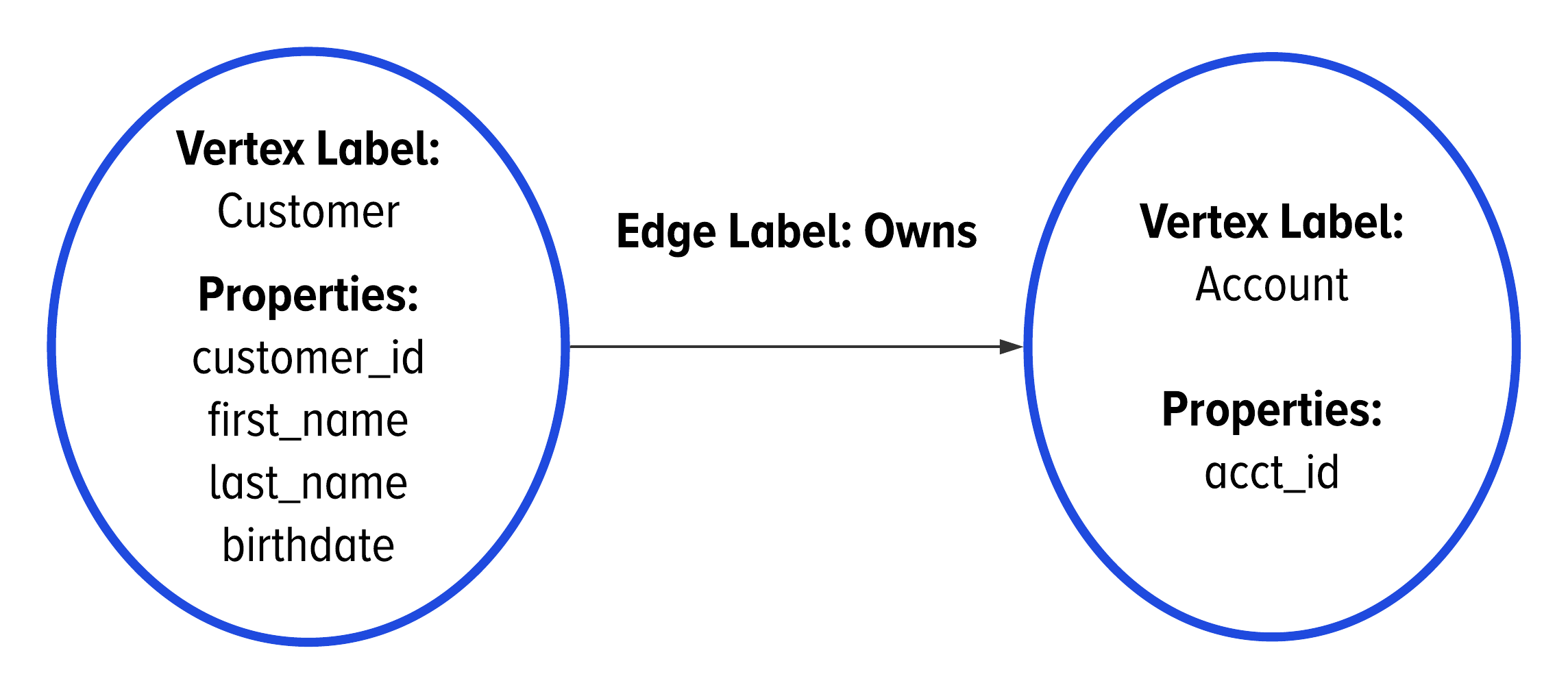
Figure 2-13. In the GSL, we use a single line to indicate when the group of adjacent vertices needs to be a set.
In order to be able to model many edges between two vertices, we need a way for one edge to be different from another edge. In Figure 2-12, we added the role property to the edge so that each edge is different. Figure 2-14 shows how we use a double line and a property value in the GSL to illustrate that we want to have at many edges between two vertices.
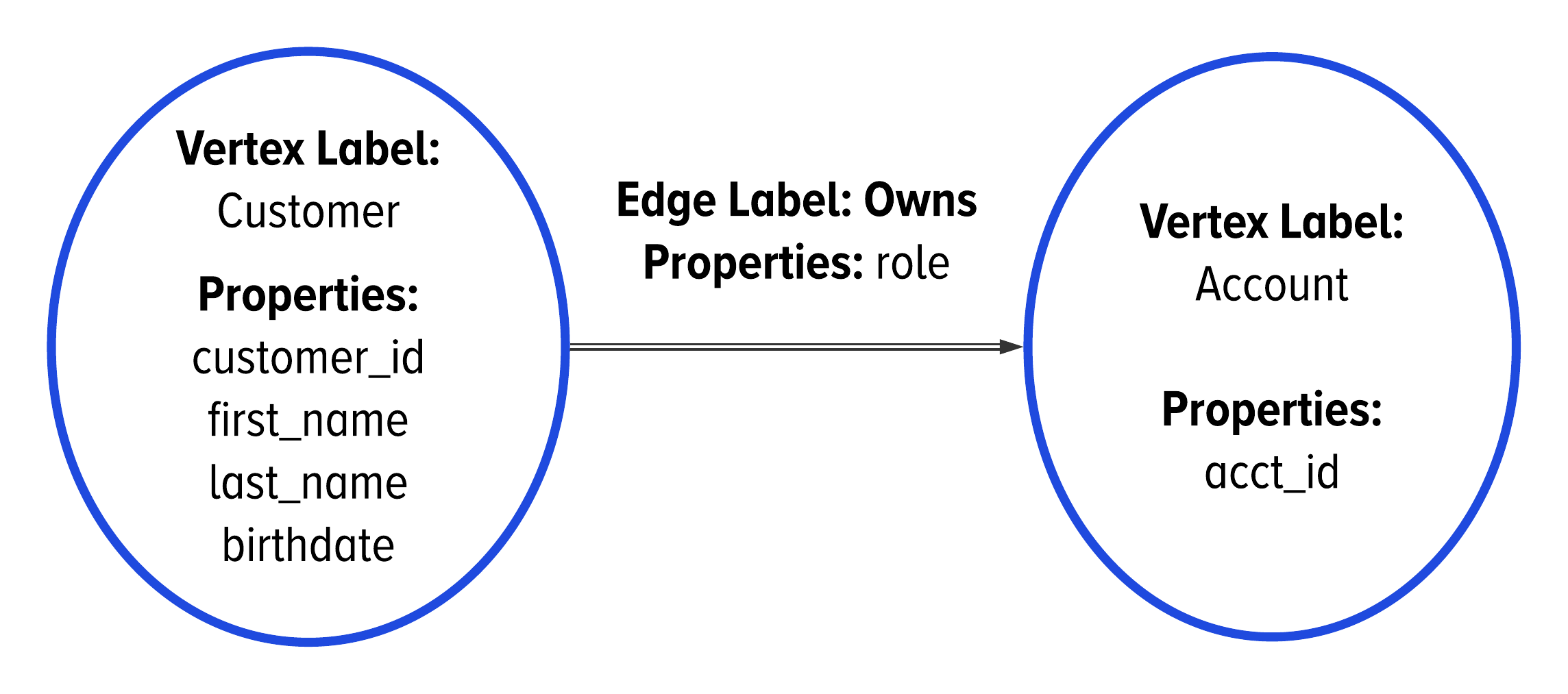
Figure 2-14. In the GSL, we use a double line to indicate when the group of adjacent vertices needs to be a collection.
The trick to understanding multiplicity lies in understanding your data. If you need to have multiple edges between two vertices, i.e. you need the group of connected vertices to be a collection rather than a set, then you need to define a property on the edge that makes it unique.
Full Example Graph Model
Using GSL, the data from Table 2-1 translates into the conceptual graph model shown below in Figure 2-15.
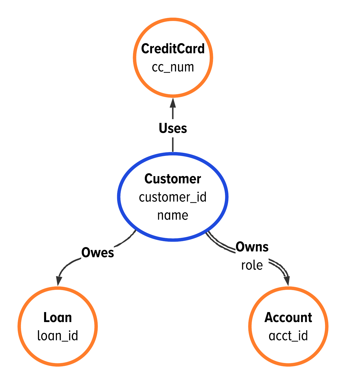
Figure 2-15. The starting point of our first example: a basic model for customer data from financial services.
We refer to the image in Figure 2-15 as a conceptual graph model. This model creates your graph database schema. This conceptual graph model shows a customer and three different pieces of data related to the customer. These four entities translate to four separate vertex labels: Customer, Account, Loan, and Credit Card.
These four pieces of data are related in three ways: customers own accounts, use credit cards, and owe loans. This creates three edge labels in the conceptual graph model: owns, uses, and owes, respectively. All three edge labels are directed; there are no bidirectional edge labels in this example data. Further, we see that the edge labels owes and owns have single cardinality wheres uses will have multiple cardinality.
The final piece of Figure 2-15 to explore are the properties shown on each vertex label in monospaced font. These are the properties that we can find in the data from Table 2-1. A Customer has two properties: customer_id and name. The Account, Credit Card, and Loan vertex labels have only one property. This property is the unique identifier for the data: acct_id, cc_num, and loan_id, respectively.
It is important to understand the difference between Figure 2-15 and the instace data we showed in Figure 2-4. Figure 2-15 shows the conceptual graph model for your database schema using GSL. Figure 2-4 shows what the data will look like in your graph database.
Relational Versus Graph: Decisions to Consider
The most difficult evaluations of relational versus graph technologies are those which intertwine techniques for database modeling with those of data analysis. We want to conclude with a few notes on each of those topics to set you up for more effective evaluation processes.
Data Modeling
Graph data modeling is very similar to relational data modeling; the main difference is in the consideration of relationships between entities. Graph technology is optimized for relationship first data organization in order to provide direct access to an entity’s relationships in the database. Given this, you will want to explore graph technology if the relationships between your entities are the most important features of your data.
In contrast to relational technology, graph technology was created to minimize the transition from mental model to data storage and retrieval. With graph technologies, the conceptual data model is the actual physical data model. That is, you don’t have to specifically do any physical data modeling as the graph database optimizes the storage and physical layout based on the logical model alone. This is achieved by storing the edges for a vertex in structures which give direct access to the edges associated to a vertex.
From our experience, the shorter translation from mental model to data storage is one of the primary reasons architects are turning from relational to graph technologies. When using graph technology, you can draw one image that represents both the conceptual understanding and physical organization of your data. This shorter interpretation from conceptual to physical data organization creates a more powerful way to envision, discuss, and apply the relationships within your data. Without graph thinking and technology, this was previously unachievable.
Understanding Graph Data
Applied graph theory empowers the appeal of using graph technology in your application. Graph technology gives you the means to understand both if and how well your data is connected together. Specifically, concepts like neighborhoods and degree open up to a new understanding about your data which is not possible with relational technologies.
The nuances between the worlds of graph schema and graph data are very important. Introducing graph technology to your team comes with a learning curve of new terms, concepts, and applications. One of the most effective ways to keep yourselves from being blocked is to understand which concepts apply to database modeling and which apply to data analysis at the application level.
Mixing Database Design with Application Purpose
From our experiences, teams often confuse concepts about graph data analysis and graph schema. It might help to draw a parallel to what this sounds like in the relational world because the differences seem so obvious from that perspective.
The parallel to relational technology highlights the differences between database applications with database schema. As we see it, interchanging terms from graph schema and graph data is the same as interchanging pie charts with foreign key constraints. Let’s unpack that.
Relational technologies are great for setting up a database that creates reports and summaries of data, like pie charts. Something like a pie chart visualizes a metric about the data. The application (the pie chart) is a completely different and an unrelated concept from relational schema design, like selecting foreign key constraints between tables.
For relational technology, the difference in this parallel is well understood. An application of your relational database is to create pie charts and the database’s schema requires designing with foreign keys to make it possible.
When getting started with graph technology, this same distinction applies. After you have set up your graph database, you use it to understand the connectivity of your data. Specifically, you can find the distance between two vertices in your graph. This is at the application level and uses data to understand the connections within the data. This is made possible by creating a graph database schema with vertex labels, edge labels, and properties.
For graph practitioners, the difference in this parallel is well understood. An application of your graph database is to calculate the distance between vertices and the database’s schema requires designing with edge labels and vertex labels to make it possible.
The important take away here is to understand the differences between creating database schema and analyzing graph data. Up until now, the flood of graph thinking has introduced many waves of terminology and complexity. From this introductory chapter, we hope to have clearly delineated the techniques for creating database models and a few for analyzing graph data.
Summary
This chapter set out to translate the concepts and terms that are used across multiple communities. Our goals for this content were to provide background and information for the following three objectives:
-
Is graph technology better for my problem than relational?
-
How do I think about my data as a graph?
-
How much do I need to learn in order to get started with graph technology?
From our experience, these three questions are the primary topics of conversation within development teams who are evaluating graph technology for their application stack.
To answer the second question, we formalized and introduced a language for creating graph database models, namely the GSL. Even though the details we have in this chapter scratch the surface for each topic area, what we have here illustrates the most vital terms and concepts to understand. Understanding these concepts will give you the ability to determine if relational or graph technology is right for your next application.
Outside of the GSL, we selected the remaining content in this chapter as the minimum topic set needed to answer the third question above. The remaining terms and topics represent the starting point for understanding data modeling, graph data, and application design in relational or graph systems. Combined with the GSL, the foundational concepts throughout this chapter represent what you need to know to get started with graph technology. At this point, you are fueled with the terminology and concepts you need to begin your first application design and evaluation.
While we have provided information for the last two questions above, we admittedly haven’t directly given you much to address our first question. This is because we can’t answer it directly for you. Your team’s need for graph technology for your application comes down to the applicability of the concepts and terms presented throughout this chapter. To boil it down: if relationships matter to your data, then graph technology will be the right answer for your team. Only you can determine that about your data.
On the other hand, we can help you navigate the use of relational or graph technology for specific use cases. The next chapter will walk you through a common starting use case where team’s typically put relational versus graph technologies to the test. Without further ado, let’s start with the foundation that companies have successfully built as the gateway to using graph data in your business: the single view of your customer.
1 Batini, Carlo, Stefano Ceri, and Shamkant B. Navathe. Conceptual database design: an Entity-relationship approach. Vol. 116. Redwood City, CA: Benjamin/Cummings, 1992.
2 Booch, Grady, James Rumbaugh, and Ivar Jacobson. The unified modeling language reference manual. Vol. 2. Reading: Addison-Wesley, 1999.