
Chapter 5. Exploring Neighborhoods in Production
When you are using DataStax Graph, you are working with graph data in Apache Cassandra. And, if you have been following along and executing the implementation details from the last two chapters, you have already been using it.
The paradigm shift from working with traditional database to working with Apache Cassandra is that we write our data according to how we are going to read it.
To illustrate how we apply this, the examples in Chapter 3 and Chapter 4 used, but skipped over, fundamental topics of working with graph data in Apache Cassandra. Concepts like edge direction and partition key design are fundamental to building a production quality, scalable, and distributed graph data model.
We are going to dig deeply into the topics of distributed data to set you up for a successful use of distributed graph technology within your production stack.
To explain what we mean by “dig deeply”, recall from Chapter 4 that we purposefully set up some traps in our example’s development. Our example built up the schema we are showing in Figure 5-1 and aimed to use queries like we have below in Example 5-1.
Figure 5-1. The developmental data model for a graph based implementation of an C360 application from the previous chapter.
There are two concepts to connect together in order to see the whole picture. First, all of our queries have been using the development traversal source, dev.V(). The development traversal source in DataStax Graph enables you to walk around your data without worry about indexing strategies. Second, our queries walk from an account vertex to transactions. If you try to run the query in Example 5-1, but switch to the production traversal source g, you will experience something like the following:
Example 5-1.
g.V().has("Customer","customer_id","customer_0").// the customerout("owns").// walk to their account(s)in("withdraw_from","deposit_to")// access all transactions
In DataStax Studio, you will see something like:
| Execution Error |
|---|
com.datastax.bdp.graphv2.engine.UnsupportedTraversalException: |
One or more indexes are required to execute the traversal |
This error is tied to the representation of graph data structures on disk. In the rest of this chapter, we take a peak under the hood to explain the why and then apply the how.
A summary of this chapter’s topics is below.
TL;DR: Understanding Distributed Graph Data in Apache Cassandra
We selected the next set of technical topics to illustrate the minimum required set of concepts for building production quality distributed graph applications. This chapter will have three main sections that align with the accompanying notebook and technical materials.
Working with Graph Data in Apache Cassandra: The first section of this chapter revisits the topics we used, but did not explain, in from Chapter 4. Here, we introduce the fundamentals of distributed graph structures to model our queries from Chapter 4. Namely, in this first section, you will learn about partition keys, clustering columns, and materialized views.
Graph Data Modeling 201: The second section applies the concepts of distributed graph structures to our second set of data modeling recommendations. We will introduce demoralization, indexing, revisit edge direction, and talk about loading strategies. These tips represent data modeling decisions that we recommend for production quality, distributed graph schema.
Production Implementation Details: The last section walks through the final iteration of our C360 example. We will explain the schema code that applies the concepts of materialized views and indexing strategies. Lastly, we will go through one last iteration of our Gremlin queries to use the new optimizations.
All together, we consider the thought process and development from Chapter 3, Chapter 4, and Chapter 5 to represent the development life cycle of designing, exploring, and finalizing the models and queries for your first application with distributed graph data.
Let’s take one last step down into the physical data layer of working with graph data in Apache Cassandra to detail our experience of building distributed graph technologies.
Working with Graph Data in Apache Cassandra
This section takes a peak under the hood to illustrate three fundamental concepts of working with graph data structures in Apache Casssandra: primary keys, clustering columns, and materialized views. Further, we are going to discuss the topics about Cassandra from a graph user’s perspective.
First, we will talk about what you need to know about vertices, and then what you need to know about edges. For vertices, you need to know about partition keys and clustering columns. For edges, you need to know about clustering columns and materialized views. Also, this isn’t a book about cassandra. We want to present what you need to know about Cassandra from the perspective of a graph user.
Let’s get started with the concept that is connecting everything together: the primary key.
The most important topic to understand about data modeling: Primary Keys
A major challenge of building a good data model within a distributed system is determining how to uniquely identify your data with primary keys.
Without detailing their purpose, you already worked with one of the simplest forms of a primary key: the partition key.
-
The partition key is the first element of a primary key in Apache Cassandra. The partition key is the part of the primary key that identifies the location of the data in a distributed environment.
From a user’s perspective, the entire partition key is required for you to be able to access your data from the system. The partition key is just the first piece of the full primary key.
-
The primary key describes a unique piece of data in the system. In DataStax Graph, a primary key can be made up of one or more keys.
You have already been using and working with primary and partition keys. In DataStax Graph, you specify the desired primary key in the schema API. We saw the simplest version of a primary key, only one partition key, in the last chapter with:
schema.vertexLabel('Customer').ifNotExists().partitionBy('customer_id',Int).// simplest primary key: one partition keyproperty('name',Text).create();
The partitionBy() method indicates the value that will be included in the label’s primary key. In this case, we only have one value, customer_id. This means that customer_id is the full primary key and partition key for the Customer vertex.
From the user’s perspective, this decision has three consequences to your application. First, the value for customer_id uniquely identifies the data. Second, your application will need the value for customer_id to read the data about the customer. We will cover the third point in a second.
As a user, these two consequences govern how you design your data’s primary and partition keys. Let’s take a look at an example. Previously, you used your primary key to look-up this data in Gremlin via:
g.V().has("Customer","customer_id","customer_0").valueMap()
which returns:
{"name":["Michael"],"customer_id":["customer_0"]}
Looking up vertices or edges by their full primary key is the fastest way to read data in DataStax Graph. This is one of the main reasons that selecting a good partition and primary key for your data is so important.
There is a third consequence of the partition key in Apache Cassandra. A vertex label’s partition key assigns your graph data to an instance within a distributed environment and different ways you can collocate your graph data. Let’s dig into the details.
Partition Keys and Data Locality in a Distributed Environment
The importance of partitioning graph data becomes even more elevated in a distributed environment.
And, we need to be pedantic about what we really mean here for a brief moment.
The word “partition” means two very different things to two different groups of people. The Cassandra’s community’s understanding of partition answers the question “where is my data in my cluster?” The graph community’s understanding of partition answers the question “how can I organize my graph data into a smaller group to minimize an invariant?”
This book applies the Cassandra community’s definition of partitioning to working with graph data. When we are referring to a partition, we are referencing data locality, or on which server your data is written to disk across your distributed system.
To illustrate how we will be using the idea of partitioning, let’s recall at some instance data for our current example.
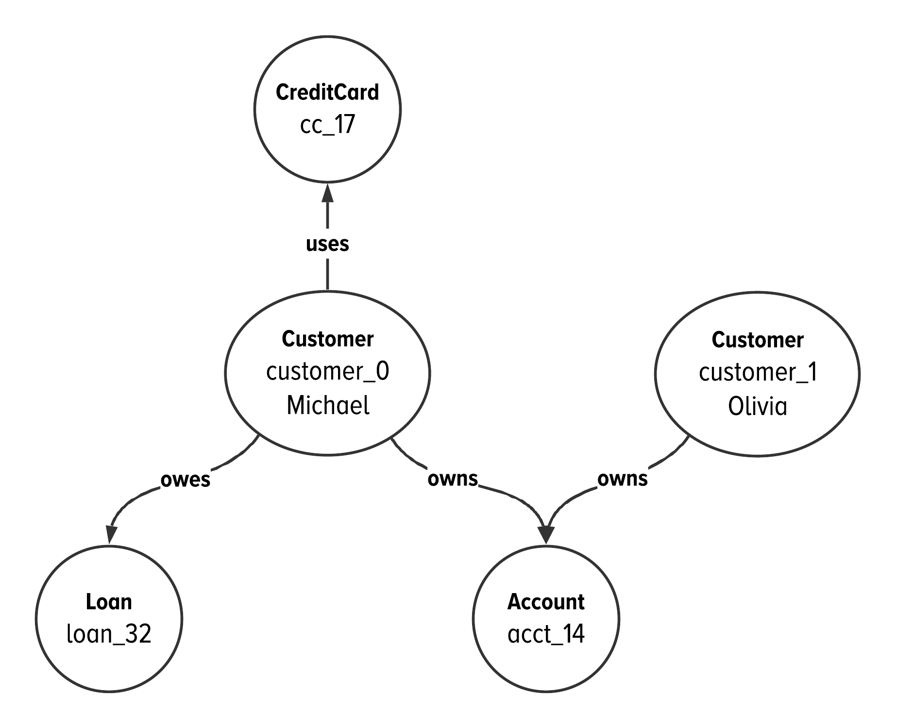
Figure 5-2. Instance data about three customers in our C360 example.
To visualize data assignment to a server (also referred to as an instance or node) in a cluster, consider you are working with a cluster of four servers running DataStax Graph in Apache Cassandra. In the upcoming Figure 5-3, we represent a distributed cluster with a circle that has four servers running Cassandra. (The eye in Figure 5-3 represents DataStax Graph in Cassandra.) Then, we can show where your graph data is written to disk by illustrating the graph data next to the server around your cluster, as we are doing in Figure 5-3.
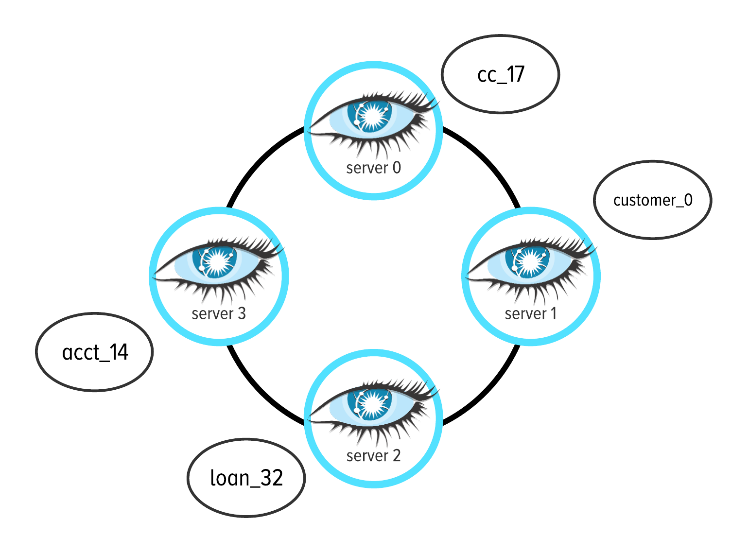
Figure 5-3. For the instance data we are working with, this image shows which server (node) each vertex is stored within a distributed cluster. The circle with four eyes represents a distributed cluster running four instances of DataStax Graph in Cassandra. The vertex for cc_17 is written to server 0. The vertices for customer_0, loan_32, and acct_14 are written to servers 1, 2, and 3, respectivley.
The ring in Figure 5-3 represents a cluster of four servers running DataStax Graph in Apache Cassandra. The instance data from Figure 5-2 is shown next to the server in the cluster where the data is physically stored. In Apache Cassandra, data is mapped to a specific server in your cluster according to its partition key.
In Figure 5-3, you see that the data for customer_0 is mapped to four different machines. The customer vertex is written to server 1, the loan vertex is on server 2, the account vertex is written to machine 3, and the credit card vertex is on machine 0.
You can think of partition keys and their association to data locality in a distributed environment as follows. Data with the same partition key is stored on the same machine. Data with different keys may be stored on different machines.
Partitioning Graph Data According to Access Pattern
With graph data, there are strategies for designing your partition keys in order to minimise the latency of your graph traversals. Different partitioning strategies affect the collocation of your data, and therefore, the latency of your query.
To minimize jumping around machines in your cluster when you are processing your graph data, you may consider a partitioning strategy which keeps all the data related to your query within the same partition. Let’s take a look at how this could work.

Figure 5-4. A visual example of partitioning graph data in a distributed system according to access pattern.
To illustrate this, Figure 5-4 illustrates a partitioning strategy according to the expected access pattern of an C360 application. The partitions are defined according to the individual customer and their data because an C360 query will typically be looking for an individual and their associated data. For our sample data, we would create partitions for each of the individuals.
Note
If you have a background in graph theory, the partitioning strategy illustrated in Figure 5-4 is similar to partitioning according to connected components.
If you have a background in working with Apache Cassandra, the partitioning strategy illustrated in Figure 5-4 follows the same practice of partitioning according to access pattern.
To implement the partitioning strategy illustrated in Figure 5-4, you would need to add the customer’s unique identifier as the partition key for every vertex label. In your schema code, that would look like:
schema.vertexLabel('Account').ifNotExists().partitionBy('customer_id',Int).clusterBy('acct_id',Int).property('name',Text).create();
Let’s think about what we are suggesting here for a moment.
It is useful to consider this partitioning strategy because it minimizes the latency of your query. All of the data for your customer centric query is collocated on the same node in your environment. This is an optimization at the physical data layer that will be advantageous when you query your data.
However, there are two reasons why this type of partition strategy will not be recommended for the queries we are exploring for our example. To see this, recall that the full partition key is required to start your graph query. The first downside to the design shown in Figure 5-4 is that you will need to know the customer’s identifier to start your graph traversal at an account.
Applying this to our example of a shared account, acct_14, brings us to another perspective. This schema design will create two vertices about acct_14 that are adjacent to two different people. This means that you won’t be able to start at acct_14 and find all customer’s which own that account. This has implications on your graph use case.
For an C360 queries we are exploring in this example, the partition strategy from Figure 5-4 doesn’t make sense. When we talk about trees in an upcoming example, however, this is a potential data model optimization to minimize query latency.
Partitioning According to Unique Key
Let’s take a look at a second strategy and compare it to collocating data according to your application’s access pattern.
Think back to the the full schema for our example and recall that each vertex label had a single, unique partition key. You can think of this as separating your graph data via the most granular division possible: the data’s most unique value.

Figure 5-5. A visual example of the different partitions within your graph data according to the vertex label’s partition key.
The graph data in Figure 5-5 would distribute the vertices across your cluster according to the partition key’s value. In this example, the data would be written to different partitions according to each vertex’s partition key. Essentially, each vertex will be mapped to a different partition because each partition key’s value is unique.
One of the draw backs to partitioning your vertices according to a unique key is that any time you need to walk through your data, you will be jumping between machines across your distributed environment. The purpose of using graph data in your application is to use the connections and relationships in your data. If you structure your graph data across a distributed environment according unique identifiers, that also means that you will (likely) be switching servers each time you need to access connected data.
Final Thoughts on Partitioning Strategies
There are benefits and drawbacks for implementing different partitioning strategies with graph data in a distributed environment. Partitioning your graph data according to access pattern creates limitations on how you can walk through connected data. On the other hand, this strategy does minimize traversal latency by collocating large components of data onto the same node.
The most common way to partition your graph data is by data’s unique identifier. This makes it easiest to plan for query flexibility, but does introduce latency to your queries due to the distributed nature of your graph. This is the approach we will use for our C360 example.
The only way to understand the implications of any partition strategy is to calculate what it would look like for your data and queries. This requires a balance between understanding the distributions in the data for the application you need to build today, and the future scope towards which you are be building.
Note
Selecting a good partitioning strategy is more tangled when we are working with graph data. Partitioning graph data around a distributed environment is synonymous with breaking up your graph data into different sections. Optimizing which data belongs to a particular section is classified as one of the hardest types of problems in computer science: an NP-Complete problem. While maybe not the best news, this helps to explain why using graph technologies in a distributed environment isn’t as simple as translating a drawing into a database.
In regards to the topic of partitioning, there are two main take aways to restate here: uniqueness and locality. In DataStax graph, your data’s partition key is its unique identifier. For fastest performance, you will want to start your graph queries by identifying pieces of data via their full partition key.
The last thing to note is that your data’s partition key determine’s its locality in your cluster. This governs exactly which machines in your cluster will store the data and the co-location of other data along side it.
Given uniqueness and locality with partition keys, let’s take a look at how edges are represented in Apache Cassandra.
Understanding Edges Part 1: Edges in Adjacency Lists
Diving into the world of graph modeling brings a large wave of terms, concepts, and thinking patterns. Now that we have the basics covered, let’s take a look at how graph data, namely the edges, can be represented on disk or in memory.
There are three main data structures for representing relationships between data: edge lists, adjacency lists, and adjacency matrices.
-
An edge list is a list of pairs where every pair contains two adjacent vertices. The first element in the pair is the source (from) vertex, and the second element is the destination (to) vertex.
-
An adjacency list is an object which stores keys and values. Each key is a vertex and the value is a list of the vertices which are adjacent to the key.
-
An adjacency matrix represents the full graph as a table. There is a row and column for each vertex in the graph. An entry in the matrix indicates if there is an edge between the vertices represented by the row and column.
To understand each data structure, let’s look at how we would map a small example of graph data into each structure.
There is a significant amount of detail illustrated in Figure 5-6. At the top, we illustrate a small example of five vertices that are connected by four edges. Direction matters when you map the data into each of the graph data structures below.

Figure 5-6. An example of three different data structures for storing edges on disk.
Let’s walk through each data structure.
On the lower left in Figure 5-6, we wrote out how the example data would be stored in an edge list. The edge list contains four entries: one entry per edge in our example data. In the center, we represent how the example data maps to an adjacency list. The adjacency list has two keys: one key per vertex with outgoing edges. The value for each key is a list of the incoming vertices the edges point to. The last data structure, shown on the far right, is an adjacency matrix. There are five rows and five columns: one for each vertex in the graph. Then, the entry in the matrix indicates if there is an edge going from the row vertex to the column vertex.
There are space and time trade-offs for each data structure. Skipping over optimizations that can be made for each individual data structure, let’s consider the complexities of each at a basic level. Edge lists are the most compressed version of representing your graph, but you have to scan the entire data structure to process all edges about a specific vertex. Adjacency matrices are the fastest way to walk through your data, but they take up an inordinate amount of space. Adjacency lists combine the benefits of each of these models by providing an indexed way to access a vertex and limit the list scans to only the individual vertex’s outgoing edges.
In DataStax graph, we use Apache Cassandra as a distributed adjacency list to store and traverse your graph data. Let’s dig into how we optimize the storage of edges on disk so that you can get the most benefit out of the sorting order of your edges during your graph traversals.
Understanding Edges Part 2: Clustering Columns
A clustering column determines a sorting order of your data in tables on disk.
You have used the concept of clustering columns when you added edge labels to your graph. Understanding clustering columns for edges, and how to use them, are our last two technical topics for this section.
We want to dig into the details of clustering columns topic because it explains two concepts at the same time. First, the technical implications of clustering columns detail exactly why the query at the beginning of this chapter returned an error. Second, clustering columns illustrate how we sort your edges in disk in an adjacency list structure to provide the fastest access possible.
You already saw an example of using a clustering column when you created an edge label:
Example 5-2.
schema.edgeLabel('owns').ifNotExists().from('Customer').// the edge labels's partition keyto('Account').// the edge labels's clustering columnproperty('role',Text).create();
Following the example in Example 5-2, we can pick out the partition key and clustering columns for our edge label:
-
The
from(Customer)step means that the full primary key of theCustomervertex will be the partition key for the edge labelowns. -
The partition key for the
ownsedge iscustomer_id. -
The full primary key for
Accountwill be the clustering column for theownsedge. -
The clustering column for the
ownsedge isacct_id.
Putting this together, we can lay out Cassandra’s table structures along side the graph schema.
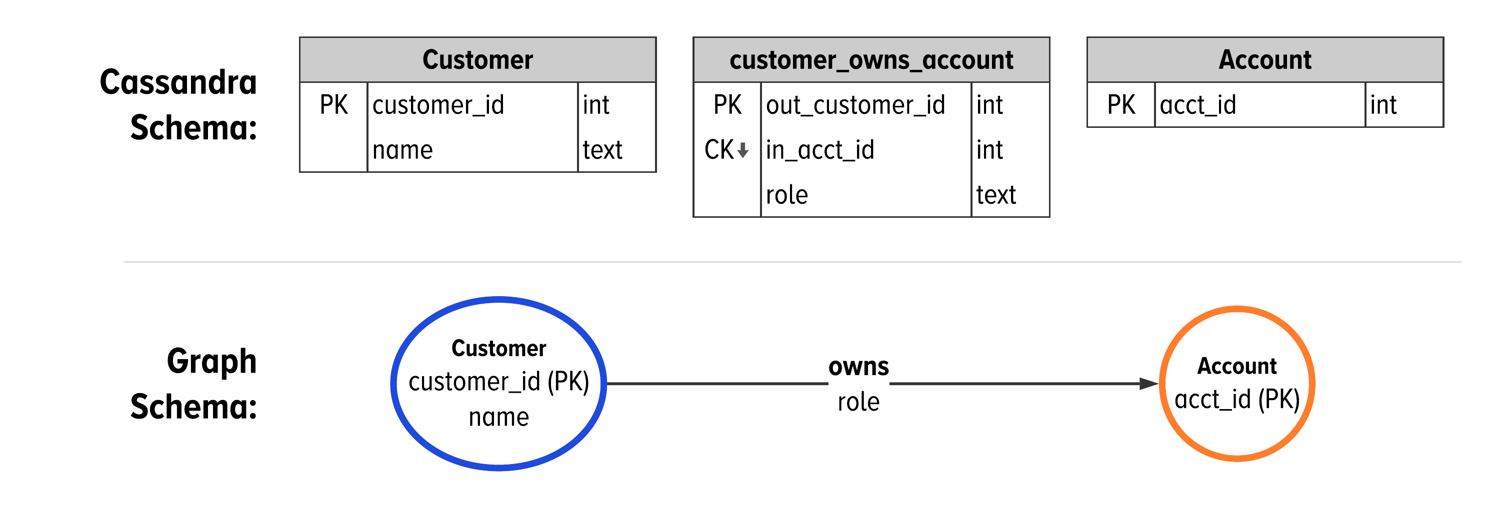
Figure 5-7. The default table structure in Cassandra for an edge between two vertices.
Figure 5-7 shows the table structures in Cassandra as they map to graph schema using the GSL. The Customer vertex creates a table with a single partition key, customer_id. The owns edge connects Customers to Accounts. The partition key of the owns edge is the customer_id. The owns edge also has a clustering key, in_acct_id, which is the partition key of the account vertex. There is a third column in the customer_owns_account table: role. This is a simple property and is not a part of the primary key. As a result, the value for role will come from the most recent write of an edge between a customer and an account.
To make this concrete, Figure 5-8 shows an example of data that follows the schema from Figure 5-7.
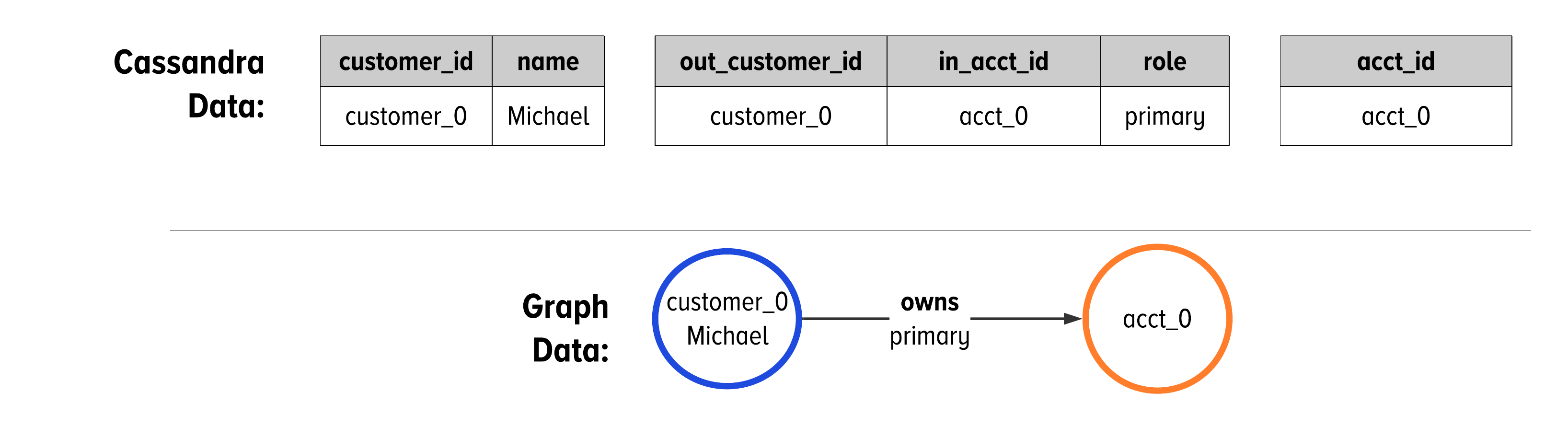
Figure 5-8. Looking at how our data from the schema in Figure 5-7 would be organized on disk and how it would be represented in DataStax Graph.
Before moving onto a different topic, there is one last idea to synthesize about clustering keys and edges in DataStax Graph. In Chapter 2, we outlined cases when you want to have many edges between two vertices. We denote this in the GSL with a double lined edge. In Cassandra, we would make that property a clustering key. Figure 5-9 shows the Cassandra schema alongside a graph schema that models adjacent vertices as a collection.

Figure 5-9. The table structure in Cassandra when we model clustering keys on edges.
Figure 5-7 shows the table structures in Cassandra as they map to graph schema using the GSL when we model the multplicity of a graph with many edges between instance vertices. The difference is in the table for the owns edge. We now have the role as a clustering key for this edge, before the clustering key for the acct_id. The schema from Figure 5-9 allows for there to be multiple edges between vertices, as we show in Figure 5-10.
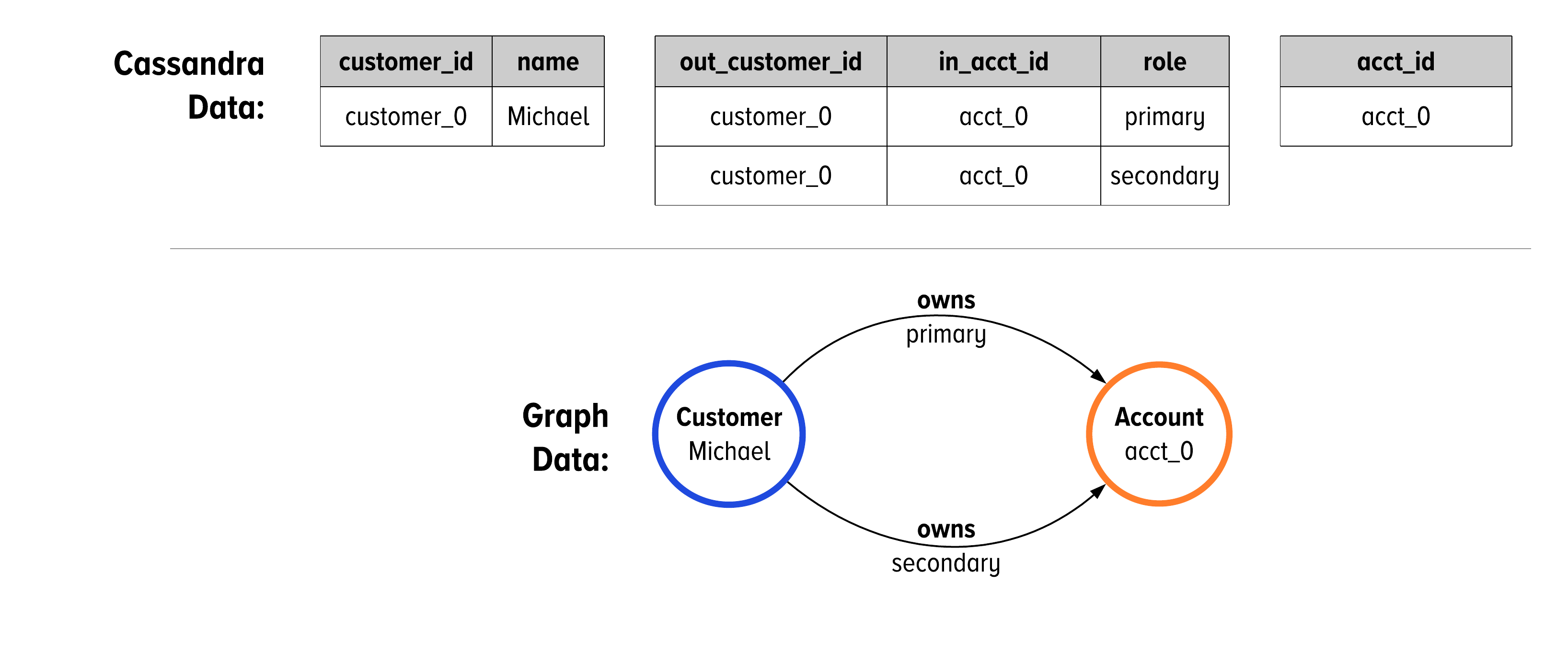
Figure 5-10. Looking at how our data from the schema in Figure 5-9 would be organized on disk and how it would be represented in DataStax Graph.
Now that we understand the structure of edges on disk, let’s visit where they will be stored within a distributed environment.
Synthesizing Concepts: Edge Location in a Distributed Cluster
Recall that the partition key identifies where the data will be written within the cluster. This means that the outgoing edges for a vertex will be stored on the same machine as the vertex itself. We previewed this in Figure 5-5 because the edges have the same color as the customer vertices; they are all orange. To illustrate what we mean, let’s take a look at the locality of edges in our cluster.

Figure 5-11. A visual example of data locality for the edges in our example.
The image in Figure 5-11 illustrates where the edges for customer0 will be stored within a distributed environment. Each of the edges will be co-located on the same machine as the vertex for customer0 because each piece of data has the same partition key: the customer_id.
The next thing to understand is how the edges are sorted within their partition. The full primary key of the to vertex becomes the clustering column(s) of the edge label. This means that the edges are sorted on disk according to their incoming vertex’s primary key.
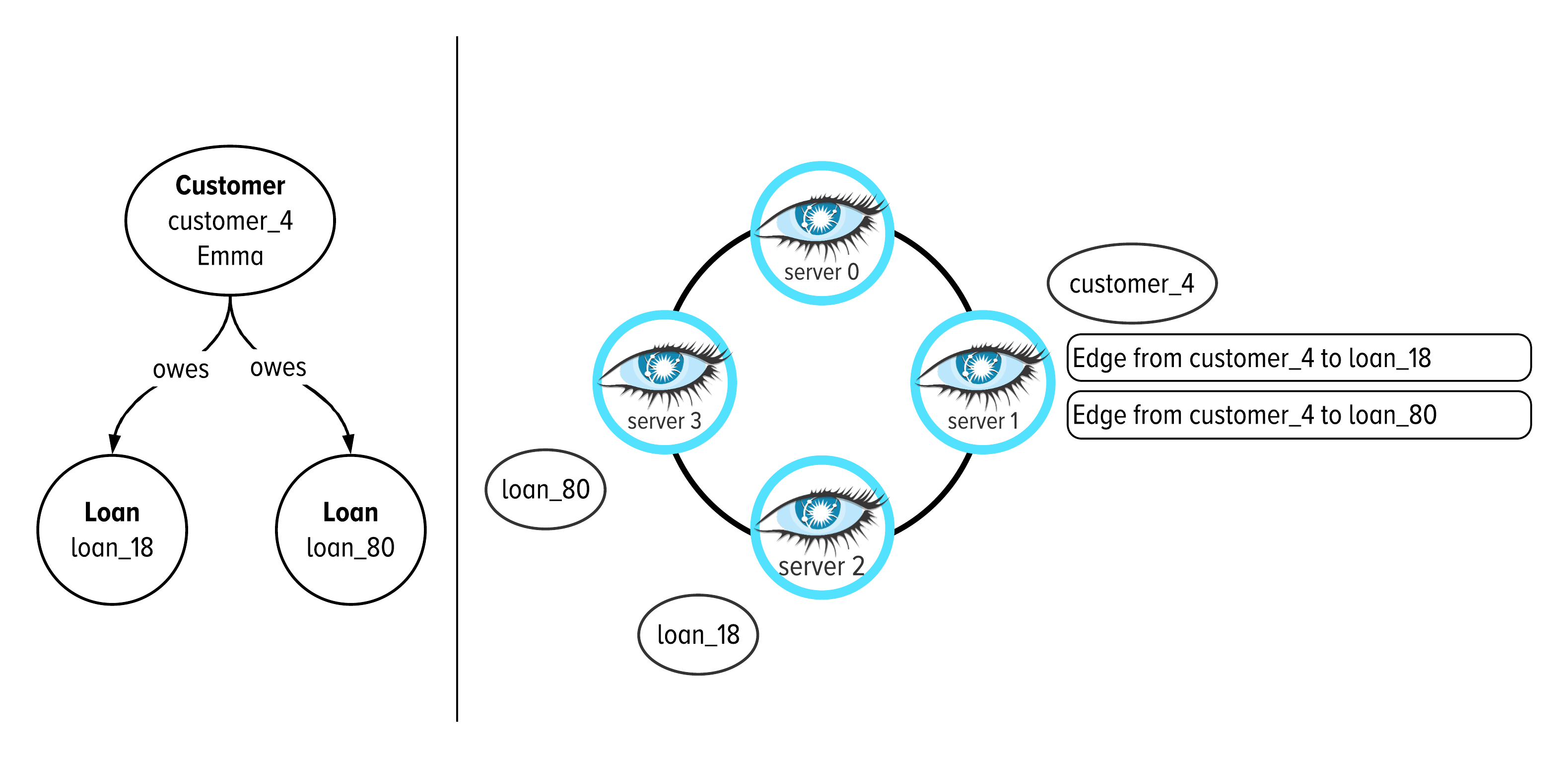
Figure 5-12. A visual example of mapping graph data, on the left, to its storage location in a distributed cluster, on the right.
The main concept to understand from Figure 5-12 is illustrated on the right. We are showing that the vertex for customer4, Emma, is written to disk on machine 1 in our cluster. Also on machine 1, we will find the outgoing edges from Emma sorted according to their incoming vertex. Emma has two loans connected to her with an owes edge. We see that on disk, these edges will be sorted according to the incoming vertex’s partition key, the loan_id. We see loan18 is the first entry and loan80 is the second entry.
You might be asking yourself: why are we getting into all this? It all comes down to the minimum requirement for accessing a piece of data in Apache Cassandra: the partition key.
Understanding Edges Part 3: Accessing Edges during Traversals
The main area you are going to feel the affects of an edge’s primary key design comes into how you access your edges. In order to use an edge, you have to know it’s partition key.
Because of this, we cannot traverse our edges in the reverse direction, yet! This is because there are no edges in the system that start with the partition key from the incoming vertex labels in our examples.
Remember our query from the beginning?
Example 5-3.
g.V().has("Customer","customer_id",0).// the customerout("owns").// walk to their account(s)in("withdraw_from","deposit_to").// access all transactions
Recalling the schema we built in the last chapter, the deposit_to edges point from a Transaction to an Account. However, Example 5-3 is trying to walk that edge in the reverse direction: from the Account and to the Transaction. Applying what we just learned about edges in DataStax graph, we know that this error happens because the edge does not exist on disk.
It was written from the transaction to the account, but not the reverse.
If we want to walk from accounts to transactions, then we need to store the edge in the other direction as well. This is not done by default in DataStax graph because of the implications to your data model, cluster load, and downstream affects of distributing your data around the system.
To create bidirectional edges in DataStax graph, this option brings us to the last technical topic for this chapter: materialized views.
Materialized Views for Bidirectional Edges
One of the main reasons engineers love Apache Cassandra is because they are willing to trade data duplication for faster data access. This is where materialized views come into play with DataStax Graph. From the user’s perspective, you think of a materialized view as follows:
-
A materalized view creates and maintains an inverse copy of the data in a separate data structure, instead of requiring your application to manually write the same data multiple times to create the access patterns you need.
Under the hood, DataStax Graph uses materialized views to be able to walk an edge in its reverse direction. Additionally, in a distributed environment, materialized views maintain data consistency between tables.
To see how to use them, let’s take a look at how to create a materialized view on the existing edge label for deposit_to.
Example 5-4.
schema.edgeLabel("deposit_to").from("Transaction").to("Account").materializedView("Transaction_Account_inv").ifNotExists().inverse().create()
This creates a table in Apache Cassandra called "Transaction_Account_inv". The partition key for this table is the acct_id. The clustering column is transactionId.
The full primary key from Example 5-4 is written as (acct_id, customer_id). This notation means that the full primary key contains two pieces of data: acct_id, and customer_id. The first value, acct_id, is the partition key and the second value, customer_id, is the clustering column.
From the users perspective, this gives us the ability to walk through the deposit_to edge from accounts to transactions. To convince ourselves of this, let’s see the edges that are stored between these two data structures by inspecting the data on disk.
We can inspect the edges on disk for the deposit_to edge label by querying the underlying data structures in Apache Cassandra. There are two tables to inspect. First, let’s look at the original table for "Transaction_deposit_to_Account" ; you can do this from DataStax Studio with the following.
select* from"Transaction_deposit_to_Account";
| out_transactionId | in_acct_id |
|---|---|
220 |
acct_14 |
221 |
acct_14 |
222 |
acct_0 |
223 |
acct_5 |
224 |
acct_0 |
The edges on disk for the materialized view of the deposit_to edge label:
select* from"Transaction_Account_inv";
| in_acct_id | out_transactionId |
|---|---|
acct_0 |
222 |
acct_0 |
224 |
acct_5 |
223 |
acct_14 |
220 |
acct_14 |
221 |
Let’s look very closely to the differences between Table 5-1 and Table 5-2. The easiest one to spot is the one transaction involving acct_5. In Table 5-1, we see that partition key for this edge is out_transactionId, which is 223. The clustering column is in_acct_id, which is acct_5.
Examine how this same edge is stored in Table 5-2, the materialized view of Table 5-1. We can see that the edge’s keys are flipped. Here, we see that partition key for this edge is in_acct_id, which is acct_5, and the clustering column is out_transactionId, which is 223. We now have bidirectional edges to use in our example.
How far down do you want to go?
We just walked through all of the technical explanations for topics in Apache Cassandra that we have planned for this book. Knowingly, the technical concepts above are a surface level introduction to the internals of Apache Cassandra presented from the perspective of a graph application engineer. There is much more under the covers for understanding partition keys, clustering columns, materialized views, and more within distributed systems.
We encourage you to go deeper and have two other resources to recommend to get you there.
First, for a full deep dive on the internals of Apache Cassandra, consider picking up a different O’Reilly book: Cassandra: The Definitive Guide: Distributed Data at Web Scale, Vol 3. by J. Carptener and E. Hewitt.
Or, for a full deep dive on the internals of distributed systems, check out the book by A. Petrov titled Database Internals: A Deep-Dive into How Distributed Data Systems Work.
Where are we going from here?
From here, we are coming back up from the internals of distributed graph data for one last pass of our C360 example. The concepts discussed introduced can be applied to give more data modeling recommendations, schema optimizations, and a few new ways to implement our Gremlin queries. So that is exactly where we are going.
The upcoming section applies our knowledge of keys and views in Apache Cassandra to data modeling best practices with DataStax Graph.
Graph Data Modeling 201
The new knowledge of the layout of vertices and edges in DataStax graph opens up more data modeling optimizations. Let’s apply our understanding of partition keys, clustering columns, and materialized views to visit our second set of data modeling recommendations.
To apply the upcoming recommendations, let’s recall where our graph schema left off:
Figure 5-13. Our development schema from Chapter 4.
Our next data modeling recommendation is:
Rule of Thumb #7
Properties can be duplicated; use denormalization to reduce the number of edges you have to process in a query.
Recalling our development schema from Figure 5-13, consider the case when an account has thousands of transactions. When we want to find the most recent 20 transactions, we need to access the account vertex by walking through to all transactions before we could subselect the vertices by time. It is pretty expensive to traverse all of the edges to access all transactions and then sort the transaction vertices.
Can we be smarter and reducing the amount of data we have to process?
We can. Specifically, we can store a transaction’s time in two places: on the transaction vertex and on the edges. This way, we can subselect the edges to limit our traversal to only the most recent 20 edges.
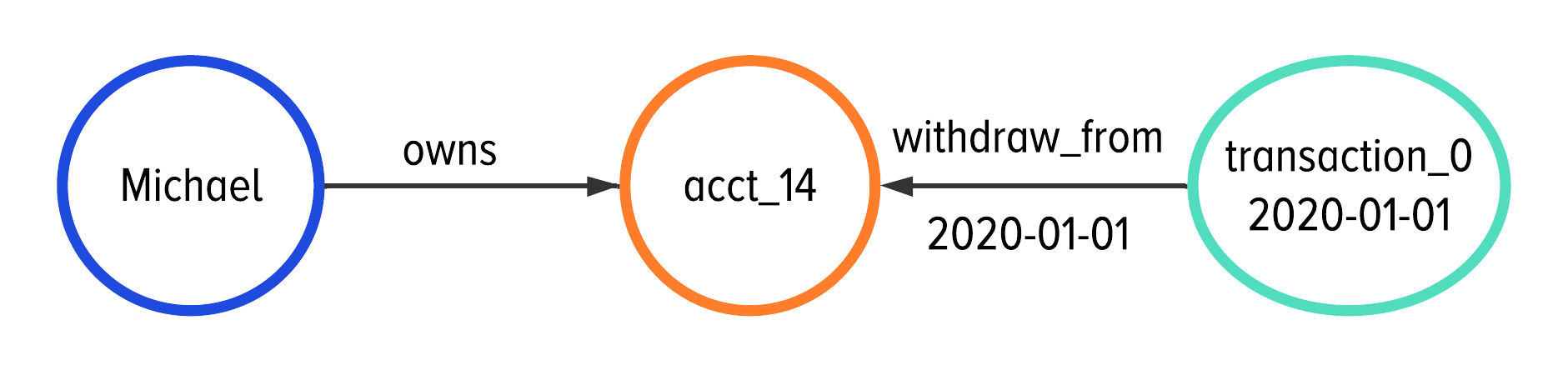
Figure 5-14. Applying denormalization to include a timestamp on the edges and vertices as an optimization to improve read performance.
In Figure 5-14, we are only showing adding a timestamp to the withdraw_from edge for simplicity; we will apply the same technique for the deposit_to and charge edge labels.
This type of optimization requires your application to write the same timestamp onto both the edge and the vertex. This is called denormalization.
-
Denormalization is the strategy of trying to improve the read performance of a database, at the expense of losing some write performance, by adding redundant copies of data or by grouping data.
Duplicating properties, or denormalization, is a very popular strategy that balances the dualities between unlimited query flexibility and query performance. On one hand, modeling your data in a graph database allows for more flexibility and easier integration of data sources. This flexibility is one of the main reasons teams are picking up graph technologies; graph technology inherently integrates more expressive modeling and query languages.
On the other hand, poor planning during development has left many teams before you with unrealistic expectations of their production graph model. They focused more on data model flexibility at the expense of query performance. Learning from their mistakes, your queries will be more performant if you take advantage of modeling tricks like denormalization.
Before you start adding properties and materialized views to all of your edges, consider our next recommendation:
Rule of Thumb #8
Let the direction you want to walk through your edge labels determine the indexes you need on an edge label in your graph schema.
With this tip, we are asking you to do do a few things here. First, we are advising you to work out your Gremlin queries in development mode first, just like we did in Chapter 4. Then, we can apply those final queries to determine only the materialized views that you need. You don’t need indexes for everything.
There are a two ways to do this in DataStax Graph. You can do it or you can tell the system to do it.
Let’s start with what this looks like if you were to figure out indexes on your own.
In order to recognize when you need an index, you have to map your Gremlin query onto your graph schema. To illustrate this, let’s use our first query and schema from development to identify where we will need an edge index.

Figure 5-15. Mapping your query onto your schema to find where you need a materialized view on an edge label.
Example 5-5.
1dev.V().has("Customer","customer_id","customer_0").// [START]2out("owns").// [1 & 2]3in("withdraw_from","deposit_to").// [3]4order().// [3]5by(values("timestamp"),desc).// [3]6limit(20).// [3]7values("transactionId")// [END]
Let’s break down what we are showing in Figure 5-15 alongside Example 5-5. We mapped each step of the query to the schema that you walk through during the query. The boxes labeled from Start to End map a green path through the schema elements to match the query to where we are walking throughout our schema.
The walk through our schema can be thought of as follows. We begin the traversal by uniquely identifying a customer, shown in the query and schema with the Start box. This is line 1 in our query. Then, we use the owns edge to access that customer’s account; this is shown in the boxes labeled 1 and 2. This is line 2 in our query. Box 3 maps together the processing and sorting of transactions. This maps to lines 3, 4, 5, and 6 in our query. End labels where the traversal stops, on line 7 of our query.
The most important concept in Figure 5-15 is at step 3. The query asks to walk through the incoming withdraw_from and deposit_to edge labels to access the Transaction vertex label. However, we are walking against the direction of the these edge labels in our schema. We highlighted this in Figure 5-15 with orange, dotted lines.
Being able to mentally see that we are walking against the direction of an edge label identifies where you need a materialized view in your graph. This is a very important concept that we hope you followed from Figure 5-15 alongside Example 5-5. We think of this last example as one of the most fundamental ah-ha moments for understanding graph data in Apache Cassandra and we hope you got there.
Finding Indexes with an Intelligent Index Recommendation System
If juggling all of this in your head is new or not natural, there is another way. You can let DataStax graph do this for you.
DataStax graph has an intelligent index recommendation system called indexFor. In order to let the index analyzer figure out what indexes a particular traversal requires, all you need to do is execute schema.indexFor(<your_traversal>).analyze() as shown below using the query we walked through in Figure 5-15.
schema.indexFor(g.V().has("Customer","customer_id","customer_0").out("owns").in("withdraw_from","deposit_to").order().by(values("timestamp"),desc).limit(20).values("transactionId")).analyze()
The output contains the following information, reformatted here to make it easier to read:
Traversal requires that the following indexes are created: schema.edgeLabel('deposit_to'). from('Transaction'). to('Account'). materializedView('Transaction__deposit_to__Account_by_Account_acct_id'). ifNotExists(). inverse(). create()schema.edgeLabel('withdraw_from'). from('Transaction'). to('Account'). materializedView('Transaction__withdraw_from__Account_by_Account_acct_id'). ifNotExists(). inverse(). create()
Essentially, Figure 5-15 and indexFor(<your_traversal>).analyze() are doing the same thing. They are mapping your traversal onto your schema to see where you need an index.
After you develop all of your queries, like we did in Chapter 4, you can use either technique to figure out where you will need indexes in your production schema.
When you are first setting up your production database, this brings us to our final recommendations:
Rule of Thumb #9
Load your data; then apply your indexes.
The application of this recommendation depends on your team’s deployment strategy. The reason we are recommending to load data before applying indexes is because this will significantly speed up your data loading process.
This is a common loading strategy because of the popularity of blue-green deployment patterns for production graph databases. If this is the type of pattern you would like to use, we recommend loading data, then applying indexes.
For a resource on deployment strategies to minimize system downtime, we recommend Continuous Delivery: Reliable Software Releases through Build, Test, and Deployment Automation by J. Humble and D. Farley.
There is one last tip to recommend:
Rule of Thumb #10
Only keep the edges and indexes that you need for your production queries.
Between development and production, you may find edge labels that you do not need for your traversals. That is expected. When you move your schema into production, get rid of the edge labels you are not going to use. Save some space on disk.
Let’s apply the new data modeling recommendations we just covered here to the development schema we built up in Chapter 4. This will be the last time we use this example and sample data before we move into different graph models in future chapters.
Production Implementation Details
The remaining implementation details in this section represent the final production version of our C360 example. The full details for reloading schema and data are contained in the accompanying notebook and technical materials.
First, we will add the required materialized views to the schema for our C360 example. Then, we will revisit and update our Gremlin queries to use the new optimizations.
Materialized Views and Adding Time onto Edges
We have a few changes to make to our development schema. First, we want to find areas when adding time onto our edges will reduce the amount of data we need to process in a query.
Let’s visualize this in Figure 5-16 for the second query of our example:

Figure 5-16. Mapping query 2 onto our development schema to see where we can use denormalization to minimize the amount of data we need to process.
Example 5-6.
dev.V().has("Customer","customer_id",0).// Startout("uses").// 1in("charge").// 2has("timestamp",// 2between("2020-12-01T00:00:00Z",// 2"2021-01-01T00:00:00Z")).// 2out("Purchase").// 3groupCount().// Endby("vendorName").// Endorder(local).// Endby(values,decr)// End
Comparing Figure 5-16 with Example 5-6 illustrates where we see the need for two production schema strategies. First, we can apply denormalization to optimize this query. Currently, time is stored only the Transaction vertex. We can reduce the number of edges required in this traversal if we denormalize the timestamp property and store it on the charge edge. This is illustrated in Figure 5-16 and Example 5-6 with label 2.
We also see in Figure 5-16 that our query walks against the direction of the charge edge. This means we need another materialized view on this edge label. The schema code is:
Traversal requires that the following indexes are created:
schema.edgeLabel("charge").
       from("Transaction").
       to("CreditCard").
       materializedView("Transaction_charge_CreditCard_inv").
       ifNotExists().
       inverse().
       create()
Following this same style of mapping, we can find three total edge labels where denormalization can optimize our queries. This optimization minimizes the amount of data a traversal has to process by sorting the edges on disk. Specifically, we can minimize the amount of data required to process our traversals if we also add the timestamp property to the withdraw_from, deposit_to, and charge edge labels.
Our Final C360 Production Schema
We have been exploring through schema, queries, and data integration to iteratively introduce and build up our c360 example. All together, the technical concepts and previous discussions bring us to our final schema for our C360 example.

Figure 5-17. The starting data model for a graph based implementation of an C360 application from the previous chapter.
The final production schema is shown in Figure 5-17. The adjustment we applied here is to denormalize and add timestamp onto the edge labels that we use in our traversals.
The final version of our edge labels for our schema code is:
Example 5-7.
schema.edgeLabel('withdraw_from').ifNotExists().from('Transaction').to('Account').clusterBy('timestamp',Text).// sort the edges by timecreate();schema.edgeLabel('deposit_to').ifNotExists().from('Transaction').to('Account').clusterBy('timestamp',Text).// sort the edges by timecreate();schema.edgeLabel('charge').ifNotExists().from('Transaction').to('CreditCard').clusterBy('timestamp',Text).// sort the edges by timecreate();
All together, we only needed the following changes from our development schema to our production schema:
-
Denormalize a property onto 5 edge labels
-
Add one materialized view to walk an edge in reverse
From here. we are ready to look at the final version of our Gremlin queries to make use of these new data structures.
Updating our Gremlin Queries to use time on edges
Now that we have updated our edge labels and indexes, let’s revisit the queries and results for each of these queries. These are the same queries we walked through in Chapter 4, but there are two changes. First, we now can use the production traversal source, g. We have moved out of development mode into writing queries against a production application. Second, we are going to update each query to use our new production schema. We will be using time on edges in addition to the materialized view.
Let’s start by revisiting Query 1.
Query 1: What are the most recent 20 transactions involving Michael’s account?
All of the work we did to set up the schema and graph data empowers the simplicity of the following query to answer our first question.
Example 5-8.
g.V().has("Customer","customer_id","customer_0").out("owns").inE("withdraw_from","deposit_to").// using the materialized view on +deposit_to+order().// sort the edgesby("timestamp",desc).// by timelimit(20).// only walk through the 20 most recent edgesoutV().// walk to the transaction verticesvalues("transaction_id")// get the transaction_ids
The results remain the same, but processed less data by sorting the edges.
"184","244","268",...
The main change in the query from Chapter 4 to this example can be seen with the addition of one character: E. The query changed from using in() to inE(). This one character change uses a materialized view and the sorted order of edges.
To dig into the details, let’s recall how we walked through this data in development mode. In Chapter 4, the in() step walked directly through edges, ignoring their direction, to the vertices and then sorted the vertex objects. That was simple enough for figuring out how to walk through our graph data.
In a production environment, we needed to ensure this query would process only the data it needs. In Example 5-8, we optimized this query by using inE(), sorting all edges by time, and only traversing the 20 most recent edges.
The sorting of all edges requires three concepts from our schema. First, we use the materialized views we built on the deposit_to and withdraw_from edge labels. Second, we use the clustering key for deposit_to because the edges are ordered on disk by time. And last, we use the clustering key for the withdraw_from edge label because these edges are also ordered on disk by time.
That is a significant amount of optimization from a small change: from in() to inE(). Let’s take a look at what we need to do to our next query to take advantage of our new schema.
Query 2: In December, at which vendors did Michael shop and at what frequency?
We are going to apply the same pattern to optimize our next query. We want to take advantage of the denormalization of time on the charge edge to minimize the amount of data we need to process. In Gremlin, this looks like:
Example 5-9.
g.V().has("Customer","customer_id","customer_0").out("uses").inE("charge").// access edgeshas("timestamp",// sort edgesbetween("2020-12-01T00:00:00Z",// beginning of December 2020"2021-01-01T00:00:00Z")).// end of December 2020outV().// traverse to transactionsout("pay").hasLabel("Vendor").// traverse to vendorsgroupCount().by("vendor_name").order(local).by(values,desc)
The results are the same as before:
{"Target":"3","Nike":"2","Amazon":"1"}
The change and optimization we applied in Example 5-9 follows the same pattern as Example 5-8. This time, we used inE() to access only incoming edges. We use the clustering key timestamp to apply a range function to the edges. Once we found all edges in a certain range, we move to the transaction vertices and continue our traversal as before from Chapter 4.
This brings us to our last query from Chapter 4.
Query 3: Find and label the transactions that David and Emma most value: their payments from their account to their mortgage loan.
Let’s think about the data this query is processing before we look at the final version of the query. In this query, we are starting from Emma and finding all withdraws from her accounts. There are no limits or time requests for this query; we want to find them all. This means that we will not be using any time ranges on the edges.
Further, every step along this query uses an existing, outgoing edge label. Because of this, we do not need any materialized views and can walk out the existing edges to satisfy this query. Therefore, we only need to switch to our production traversal source, and this query will be ready to go.
Example 5-10.
g.V().has("Customer","customer_id","customer_4").out("owns").in("withdraw_from").as("transactions").out("pay").has("Loan","loan_id","loan_18").select("transactions").property("transaction_type","mortgage_payment").values("transaction_id","transaction_type")
The results look exactly as before from Chapter 4:
"144","mortgage_payment","153","mortgage_payment","132","mortgage_payment",...
With Example 5-10, we have concluded the transformation from development to our production schema and queries. We encourage you to apply the thought process of shaping query results from “Advanced Gremlin: Shaping Your Query Results” to create more robust payloads and data structures to share within your application.
Moving onto More Complex, Distributed Graph Problems
We consider the transition from Chapter 4 to the topics and production optimizations presented here in Chapter 5 to be this final stage of learning how to work with graph data in Apache Cassandra. Along the way, you experienced limitations followed by their resolution. We will see more of that as we go along, but in shorter iterations.
Our First 10 Tips to get from Development to Production
Throughout the content in the last two chapters, we presented data modeling tips for mapping your data into a distributed graph database. In this chapter, we augmented those tips with specific ways to optimize your production graph database. Let’s revisit all 10 tips to recall the journey we went through from development to production.
-
If you want to start your traversal on some piece of data, make that data a vertex.
-
If you need the data to connect concepts together, make that data an edge.
-
Vertex-Edge-Vertex should read like a sentence or phrase from your queries.
-
Nouns and concepts should be vertex labels. Verbs should be edge labels.
-
When in development, let the direction of your edges reflect how you would think about the data in your domain.
-
If you need to use data to sub-select a group, make it a property.
-
Properties can be duplicated; use denormalization to reduce the number of edges you have to process in a query.
-
Let the direction you want to walk through your edge labels determine the indexes you need on an edge label in your graph schema.
-
Load your data; then apply your indexes.
-
Only keep the edges and indexes that you need for your production queries.
These ten tips are foundational to starting over with a new data set and use case. We will be applying them repeatedly in the coming chapters. And, we will find more to add to this ongoing list as we explore different common structures for distributed graph applications.
From here, we think you are ready to tackle deeper, and more complex graph problems like paths, recursive walks, collaborative filtering, and more.
The most advanced graph users today are those who are willing to learn from from trial and error. We have collected what they have learned so far and will be walking you through those details within the context of new use cases in the coming chapters.
As we see it, gaining traction with new technology and new ways of thinking is a journey. So far, we presented the major foundational milestones others have reached so far. From here, you are ready to come along with us and apply graph thinking in production applications to solve complex problems.
Next, we’ll look at one of the most popular ways people extend graph thinking into their data in Chapter 6. We will solve a complex problem found at the intersection of edge computing and hierarchical graph data in a self-organizing communication network of sensors.