CHAPTER 3

YOUR MORTGAGE

The Real Cost of Buying Property

What does a property cost? This is one of the most important questions investors ask, and, just as a stock market investor is interested in the price per share, real estate investors need to know how much their investments will require in capital.

This seemingly straightforward question is actually far more complex. Because you will probably be financing a major portion of the total purchase price, your real cost is not the sale price of the property but the total you pay over many years. Cost has more to do with your interest rate than with the price the seller wants.

For example, a 30-year mortgage is a common device for financing an investment property. If you buy a rental property for $240,000 and make a down payment of $96,000, you will finance the balance of $144,000. If you make payments over 30 years, what is your total cost going to be (assuming you keep the property that long)? If your interest rate is 5.5 percent, the total 30-year payments come to $294,343, more than twice the borrowed amount of $144,000.

Now consider the difference it would make if you could get a loan at 5.0 percent. You would save $16,029 over 30 years with this lower interest rate. This significant difference makes the point: You are better off negotiating a small advantage in financing than you are getting a reduced price on the property. A lot of emphasis is placed on getting a bargain; you might be able to whittle an asked price of $240,000 down to $230,000. But if you concentrate on this price difference but fail to shop for the best mortgage deal, it could be a mistake.

This chapter explores the realm of the real cost of property, resulting from the effects of compounded interest. The time value of money (the value based on how interest compounding affects your cost) is where the real cost of property is to be found. The first step is to calculate how value is accumulated over time with compound interest, as in a savings account. This leads to the opposite of accumulation, the payments made on a debt. By understanding how to calculate present value, you gain deeper insight into how mortgage acceleration works.

THE TIME VALUE OF MONEY

The long-term effects of small changes in interest rates are important in shopping for a good mortgage deal. You can also drastically reduce the overall cost of interest by making small prepayments on a mortgage. Later in this chapter, the dramatic effects of making extra payments to principal (a process called mortgage acceleration) is demonstrated.

Interest calculations show how the amount of interest accumulates over time. Most people are familiar with interest as it relates to a personal savings account. The same effects that you profit from by leaving money in such an account (in which money grows) also works for lenders. Thus, the payments you make on your mortgage reduce the debt only gradually, because most of your payments constitute interest. In fact, on average, a 30-year loan is paid down to one-half only at the end of the 25th year; the remaining half gets paid off in the last five years.

SIMPLE INTEREST

The first calculation is for simple interest, which is interest based on the nominal (or stated) rate per year. Three elements are always involved in interest calculations: principal, interest rate, and time. Simple interest is the interest you pay without any compounding.

•Formula: Simple Interest

P * R = I

where:

P	= principal
R	= interest rate
I	= interest

•Excel Program: Simple Interest

A1:	principal
B1:	interest rate
C1:	= SUM(A1*B1)

This is a straightforward formula. If the principal amount is $1,000 and interest is 4 percent, simple interest is:

$1,000 * .04 = $40.00

In calculating percentages, convert the stated percentage of interest to a decimal form to perform the multiplication function. To calculate the decimal equivalent of a percentage, divide the interest rate by 100.

•Formula: Conversion, Percentage to Decimal

R ÷ 100 = D

where:

R	= interest rate
D	= decimal equivalent

•Excel Program: Conversion, Percentage to Decimal

A1:	interest rate
B1:	= SUM(A1/100)

For example, the interest rate of 4 percent is converted to decimal equivalent using this formula:

4% ÷ 100 = 0.04

COMPOUND INTEREST

It is important to know the calculation for simple interest, even though it is rarely used. It serves as the building block for the more common calculation of compound interest. Compounding may occur in many different ways: daily, monthly, quarterly, semiannually, or annually.

Daily compounding can be done in two ways. The number of days to use may be 365 (days in the year) or 360. When 360 days are used, every month is assumed to contain 30 days; so the monthly interest would be the same each month, even though the number of days varies. Daily interest is used for some types of savings accounts. The formula used for daily compounding generally is based on the use of 365 days.

•Formula: Daily Compounding

R ÷ 365 = i

where:

R	= annual interest rate
I	= daily rate

•Excel Program: Daily Compounding

A1:	= annual interest rate
B1:	= SUM(A1/365)

For example, if the annual rate of 4 percent were compounded daily, the daily rate is:

0.04 ÷ 365 = 0.0001096

Total interest would next be calculated by adding 1 to the daily rate and multiplying it by itself for the number of days. For example, if you wanted to know the interest for 11 days using a daily rate of 4 percent, the calculation is:

(1 + 0.0001096)¹¹ = 1.0012063

Over 11 days, the $1,000 of principal would grow to:

1.0012063 * $1,000.00 = $1,001.21

While the 4 percent daily compounding produces only $1.21 over 11 days, the annual interest would be slightly higher than simple interest. The compounding would add money to the fund at a higher rate. The calculation of interest on a single deposit is called the accumulated value of 1.

•Formula: Accumulated Value of 1

(R + 1)ⁿ * P = A

where:

R	= periodic interest rate
n	= periods
P	= principal amount
A	= amount accumulated (principal plus interest)

•Excel Program: Accumulated Value of 1

A1:	principal amount
A2	Interest rate
A3:	Number of periods per year
A4:	Number of years
B4:	= FV (r/n,1*r,,–1000)

The Excel formula uses the shortcut “FV” for computation of future value. In the example of a single initial amount (in this case $1,000), the formula uses the abbreviated value of =FV(0.04/365,1*365,,−1000) in cell B4 to yield the result of $1,040.81. Thus, daily compounding yields more than the simple interest of $40. This can be proven by first calculating the daily rate (dividing 0.04 by 365); next, adding 1; and finally, multiplying the result by itself 365 times.

The periodic interest rate is always calculated by dividing the stated annual rate by the number of periods. In the case of daily interest, the periodic rate equals the rate divided by either 365 or 360; the monthly periodic rate is determined by dividing the annual rate by 12; the quarterly rate, by dividing by 4; and the semiannual rate, by dividing by 2.

•Formula: Periodic Rate

R ÷ P = i

where:

R	= annual interest rate
P	= number of periods
i	= periodic interest rate

•Excel Program: Periodic Rate

A1:	annual interest rate
B1:	number of periods
C1:	= SUM(A1/B1)

A process similar to the calculation for daily compounding is involved with monthly compounding, but because there are only 12 months in a year, the number of calculations is lower.

•Formula: Monthly Compounding

R ÷ 12 = i

where:

R	= interest rate
i	= monthly rate

•Excel Program: Monthly Compounding

A1:	principal amount
A2:	Interest rate
A3:	12
A4:	Number of years
B4:	=FV(0.04/12,1*12,,−1000)*

*In this example, the assumed principal amount is $1,000 in cell B4. This should be adjusted to the correct value. In addition, the use of “1” limits the calculation to monthly compounding for only one year.

Just as the result of the daily compounding formula produced the daily rate, this formula provides the monthly rate. The same process—using the formula to calculate interest for the number of periods—is used for monthly compounding. For example, if you are working with 4 percent compounded monthly, you calculate the one-month rate as:

0.04 ÷ 12 = 0.0033333

Next, add 1 to the monthly factor and raise it exponentially by the number of months involved. For example, to figure a $1,000.00 fund’s balance at 4 percent after five months compounded monthly, the formula is:

(1 + 0.0033333)⁵ = 1.0167780

The dollar amount is:

1.0167780 * $1,000.00 = $1,016.78

The annual interest for a full 12 months using this illustration is shown in Table 3.1.

Table 3.1: Monthly Compounding, One Year

Monthly compounding of 4 percent interest yields interest at the rate of 4.07411 percent per year because of the compounding effect. This is a small difference, but it accelerates over many years. And that is the primary point to remember about compounding: It accelerates as time goes by.

With interest compounded on a quarterly basis, compounding occurs four times per year. This produces a somewhat smaller yield than monthly compounding because there are fewer periods.

•Formula: Quarterly Compounding

R ÷ 4 = i

where:

R	= interest rate
i	= quarterly rate

•Excel Program: Quarterly Compounding

A1:	interest rate
B1:	= SUM(A1/4)

With the example of a 4 percent rate and a $1,000 deposit, the periodic rate is computed by dividing 4 percent by the number of periods:

0.04 ÷ 4 = 0.01 per quarter

The compounded annual rate is computed for each quarter using these formulas:

First quarter (1 + 0.0100000)1	= 1.010000
Second quarter (1 + 0.0100000)2	= 1.020100
Third quarter (1 + 0.0100000)3	= 1.030301
Fourth quarter (1 + 0.0100000)4	= 1.040604

And to calculate the fund’s balance by quarter, based on a $1,000 principal:

First quarter 1.010000 * $1,000.00	= $1,010.00
Second quarter 1.020100 * $1,000.00	= $1,020.10
Third quarter 1.030301 * $1,000.00	= $1,030.30
Fourth quarter 1.040604 * $1,000.00	= $1,040.60

Quarterly compounding of 4 percent results in an annual rate of 4.0604 percent.

Semiannual compounding follows the same pattern, but there are only two periods per year. Thus, the 4 percent rate is cut in half for each semiannual period, to 2 percent:

First half (1 +0.0200000)1	= 1.020000
Second half (1 + 0.0200000)2	= 1.040400

•Formula: Semiannual Compounding

R ÷ 2 = 1

where:

R	= interest rate
i	= semiannual rate

•Excel Program: Semiannual Compounding

A1:	interest rate
B1:	= SUM(A1/2)

With only two compounding periods per year, semiannual interest of 4 percent results in an annual rate of 4.04 percent.

The last method of compounding is annual. There is only one period per year, so a single compound period at 4 percent produces the nominal rate, or 4 percent per year. However, there is an important distinction to be made. With simple interest, the annual rate is 4 percent every year, without variation. In the case of annual compounding, subsequent years would see increased interest. The 4 percent rate creates annual compounding over several years.

•Formula: Annual Compounding

(R + 1)^y = i

where:

R	= interest rate
y	= number of years
i	= accumulated interest

For example, annual compounding of 4 percent over three years results in total interest of:

(1 + 0.04 )³ = 1.1248640

And with a beginning balance of $1,000.00, the value would grow at 4 percent over three years to:

Year 1:	$1,040.00
Year 2:	$1,081.60
Year 3:	$1,124.86

The preceding illustrations of compounding assume that a beginning balance of $1,000.00 is being used. The value accumulates based on a single initial deposit. So the accumulated value of 1 is a starting point for next calculating the accumulated value of 1 per period. For example, what happens to the calculated interest rate when additional funds are put into the account regularly? This is similar to the way mortgage payments are made: one payment per month. This discussion begins with a savings illustration to demonstrate how the calculation builds upon the previous examples.

As a mortgage borrower, you make payments; but if you were saving, you would calculate the future value of a series of deposits—such as money added to a savings account over time if you deposited the same amount each month. The formula needs to answer the mathematical question, What will a series of deposits be worth after n periods, assuming R interest? The formula for calculating interest on accumulated value is:

(1 + R)ⁿ =A

In this calculation, R is the interest rate, n is the number of periods, and A is the value after time has passed. However, when a series of deposits is involved, you need to figure out the accumulated value per period, and the formula has to take into account the additional funds added in.

•Formula: Accumulated Value of 1 per Period

{D [(1 + R)ⁿ – 1 ] ÷ R} * P = A

where:

D	= periodic deposit amount
R	= periodic interest rate
n	= number of periods
P	= principal
A	= accumulated value of 1 per period

To reduce this calculation to an Excel spreadsheet, the useful “FV” function simplifies the process. For accumulated value of 1 per period, all of the information is included in a single line of programming. The elements include the interest rate, number of periods per year (12 for monthly compounding, 4 for quarterly, 2 for semiannual, and 1 for annual), and the amount of periodic deposit. The following Excel programs assume 4 percent interest with $100 in period deposits, all over three years. Thus, monthly deposits include 36 deposits of $100, and annual deposits have only three periodic deposits.

•Excel Programs: Accumulated Value of 1 per Period

FV(r/n,y*d)

where:

r	= interest rate
n	= number of periods per year
y	= number of years
d	= amount of periodic deposits
Monthly:	= FV(4%/12,3*12,100)
Quarterly:	= FV(4%/4,3*4,100)
Semiannually:	= FV(4%/2,3*2,100)
Annually:	= FV(4%/1,3*1,100)

For this example of 4 percent interest and periodic payments of $100, the outcomes can also be expressed with the following formulas:

Monthly:

$100 [(1 + 0.00333)36 – 1] ÷ 0.00333

= $3,818.16

Quarterly:

$100 [(1 + 0.01)12 – 1] ÷ 0.01

= $1,268.25

Semiannually:

$100 [(1 + 0.02)6 – 1] ÷ 0.02

= $630.81

Annually:

$100 [(1 + 0.04)3 – 1] ÷ 0.04

= $312.16

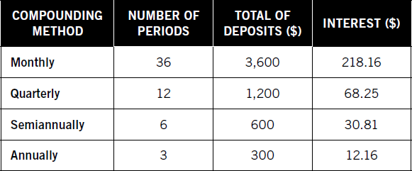
The totals using different compounding methods are based on different numbers of periodic deposits as well as different periodic rates. Breaking this down for the three-year period looks like the summary in Table 3.2.

Table 3.2: Compounding with Accumulated Value of 1 per Period

PRESENT VALUE: ITS MEANING AND CALCULATIONS

You have just seen how money accumulates with compound interest—for example, how money grows in a savings account if you make deposits over a period. A savings account may begin with modest interest, but over many years, the rate of growth accelerates because you earn interest on interest—compound interest. So interest on a single payment into a savings account or on a series of payments can be calculated to determine the future value of an account using the formulas for accumulated value.

Ultimately, a series of present-value calculations is required to figure out how a loan is amortized over many years. The tables of loan payments found in Appendix C make this easier, and you can also make good use of free online mortgage calculators. The following present-value exercises are provided to show how the formulas work, in the belief that it is important to understand where these conclusions come from; knowing how long-term interest is calculated is important to every real estate investor.

Present value shows you what happens when you pay money to a lender or when you need to save money today to arrive at a desired balance in the future. The present value of 1 is the amount required today to reach a required sum in the future, based on the interest rate and the time involved. You need to understand how this calculation works because it is needed to calculate mortgage payments.

You would use this calculation if you wanted to save up money to use in the future. For example, how much do you need to put in the bank in order to have a desired amount in the future, based on the interest rate and the amount of time involved? Using the present value of 1, you calculate how much you need to save now.

•Formula: Present Value of 1 per period

1 ÷ (1 + R)ⁿ = P

where:

R	= periodic interest rate
n	= periods
P	= present value factor

To reduce the present value of 1 to an Excel spreadsheet, use the “PV” function in Excel. All information is entered into a single entry. The elements are the periodic interest rate, number of periods, starting point (represented by zero to calculate a beginning point), and the desired future value. So a 4 percent assumption based on monthly, quarterly, semiannual, or annual compounding, over three years, varies in order to accomplish a future value of $1,000.

•Excel Program: Present Value of 1

=PV(r,p,0,FV)

where:

r	= interest rate
P	= number of periods
0	= starting point (beginning of period)
FV	= future value
Monthly:	= PV(0.333%,36,0,1000)
Quarterly:	= PV(1%,12,0,1000)
Semiannually:	= PV(2%,6,0,1000)
Annually:	= PV(4%,3,0,1000)

The outcomes of the above calculations are:

Monthly:	= PV(0.333%,36,0,1000) = $887.20
Quarterly:	= PV(1%,12,0,1000) = $887.45
Semiannually:	= PV(2%,6,0,1000) = $887.97
Annually:	= PV(4%,3,0,1000) = $889.00

The next step in this series of calculations is the sinking fund payment. As in the previous calculation, you need this step to figure out mortgage payments needed later. A sinking fund is the series of payments you need if you are to get to a target amount in the future. Returning to the previous example, in which you want to save up a fund worth $1,000 at the end of four years, how much do you need to save each quarter (assuming 3 percent compounded quarterly) to end up with $1,000 at the end of three years?

•Formula: Sinking Fund Payments

1 ÷ [( 1 + R )ⁿ ÷ R] = S

where:

R	= periodic interest rate
n	= number of periods
S	= sinking fund factor

•Excel Program: Sinking Fund Payments

= FV(r, n, p,0,0)

where:

R	= periodic interest rate
N	= number of periods
0	= first zero is equal to PV, second zero is type and indicates payments made at the end of each period; change last zero to 1 for payments at the beginning of each period

For example, assuming 4 percent nominal rate, the quarterly periodic interest rate is 1 percent. Over three years in which $100 is deposited at the beginning of each quarter, 12 quarters are involved. The Excel formula for this example is:

=FV(1%,12,100,0,0)

This produces an ending balance of $1,268.25.

The next calculation in this series is called the present value of 1 per period. This is the required deposit to be made today, based on an interest rate and compounding method, to make a series of future withdrawals, quite different from a series of deposits to accumulate a target dollar amount. While this is commonly used in long-term calculations for retirement income, for example, it also applies in real estate applications. For example, let’s assume you want to put aside money to make monthly payments of $1,000 per month over the next four months for the combination of insurance and taxes due on a rental property. You will remove money from another account and set it aside for this, but the exact amount needed each month is figured using the present value of 1 per period. While this calculation itself is not essential for real estate investing activity, it is a component of the calculation for mortgage amortization.

•The formula for the present value per period is:

{1 – [1 ÷ (1 + R)ⁿ]} ÷ R = W

where:

R	= periodic interest rate
n	= number of periods
W	= withdrawal amount

Applying this formula, you further assume that you will earn interest at 6 percent, compounded monthly, which is .005 percent per month:

{1 – [1 ÷ (1 + .005)4]} ÷ 0.005

= 3.95050

Multiplying this factor by the required series of $1,000 withdrawals gives:

3.95050 * $1,000 = $3,950.50

You need to deposit $3,950.50 into an account today to fund withdrawals of $1,000 per month for the next four months. This is an abbreviated and simplified example of how the present value of 1 calculation is performed.

The previous formulas are used as part of the equation for figuring out the required amortization payment on a long-term mortgage loan. The formula provides an answer to the question, What amount of equal payments have to be made each period to retire a debt over a specified number of periods, given the rate of interest and the compounding method?

•Formula: Amortization Payment

B (1 ÷ Pⁿ) = A

where:

B	= original balance of the loan
P	= present value of 1 per period
n	= number of periods
A	= amount of payment per period

•Excel Program: Amortization Payment

=PMT(R/P,T,B)

where:

PMT	= payment
R	= annual rate
P	= number of payments per year
T	= total number of payments
B	= amount borrowed

Example: 5 percent monthly payments for 30 years (360 months) and a loan of $100,000

Formula:

=PMT(0.05/12,360,100000)

The formula in the example above yields an answer of $536.82. This is the amount to be paid each month to retire a 30-year mortgage paid monthly at 5 percent.

The typical mortgage debt is calculated over a long term, such as 30 years (360 months), with interest computed monthly. Thus, performing this calculation by hand would be exceptionally complex, which is why amortization tables are so useful.

Amortization tables may be found in books identifying interest rate and term in years. Any number of online calculators simplify the process as well.

CALCULATING APR

Lenders and investors use specific terminology in discussing interest rates and calculations. These are important because their definitions explain how interest is actually calculated.

The annual percentage rate (APR) is confusing to many real estate investors because lenders calculate this in a variety of ways. As a general rule, the APR includes the stated annual rate plus points and other fees that are included in the loan. These fees may include not only points but prepaid interest, loan processing fees, underwriting fees, and private mortgage insurance. Lenders may also include loan application fees and, if applicable, credit life insurance premiums. However, because the calculation varies from lender to lender, you need to first determine which fees a particular institution includes in the APR.

The annual percentage rate includes the compounding effects of period interest, as well as additional fees. A distinct calculation is the actual percentage rate, which is the annual interest without other fees included. To calculate this, first figure out the periodic interest rate, then multiply the periodic rate by the number of periods in the year. For example, monthly compounding involves 12 annual periods:

•Formula: Annual Percentage Rate

[( i ÷ P ) + 1]ⁿ – 1 = R

where:

i	= annual interest rate
P	= number of periods
n	= number of periods per year
R	= annual percentage rate

•Excel Program: Annual Percentage Ratio

General formula: =RATE(T,-M,B)*12

where:

T	= total number of payments
M	= monthly payment
B	= amount borrowed

Example: = RATE(360,-536.82,100000)*12

Based on assumed 360 payments (30 years), monthly payments of $536.82, borrowed $100,000, multiplied by 12 for annual rate

The accumulated value and present value calculations are significant because they show how interest accumulates over time. This explains why it takes 30 years to pay down a loan and why you end up paying more than twice the loan amount.

The process of paying a loan all the way until it is paid off is called full amortization. This is different from other types of loan arrangements. For example, an interest-only arrangement reduces payments but does not pay down any of the loan. Some loans are negotiated with payments equal to full amortization, but with an earlier due date. This requires payment of a balloon payment or refinancing of the amount borrowed. So there are many different types of mortgage arrangements. The term creative financing often means that a lender has devised a way to qualify a borrower; in other cases, it actually means “expensive financing.”

WHAT PROPERTY REALLY COSTS

You can easily prove that the real cost of property is far higher than the purchase price. You simply need to check the required payment from a loan amortization schedule and multiply that by the months involved. To calculate the total cost of a loan, add the down payment to the total of payments.

•Formula: Cost of Financed Property

( P*M ) + D = C

where:

P	= monthly payment
M	= number of months in loan term
D	= down payment
C	= total cost of property

•Excel Program: Cost of Financed Property

A1:	monthly payment
B1:	number of months
C1:	down payment
D1:	= SUM(A1*B1)+C1

For example, if the price you pay for a property is $150,000 and you make a $50,000 down payment, you finance the balance of $100,000. At 6 percent, your monthly payment will be $599.55 for 30 years, or 360 months. Applying the formula:

($599.55 * 360) + $50,000 = $265,838.00

Lenders may offer a reduced interest rate in exchange for higher down payments. For example, consider the difference it makes if you increase a down payment to $60,000 and finance $90,000 at 5 percent. That reduces the monthly payment to $483.14 and the total cost to:

($483.14 * 360) + $60,000 = $233,930.40

This change reduces the monthly payments by $116.41 and the overall cost by $31,907.60. The savings are even greater when the repayment period is lowered. For example, if you were able to pay off the same $90,000 loan in 25 years instead of 30, the payments would be $526.13 and the total cost would be:

($526.13 * 300) + $60,000 = $217,839.00

LOWERING THE TOTAL COST OF A PROPERTY

The lower the interest rate and the faster the loan is repaid, the lower the overall cost of property. This has to be balanced against the affordability of payments. In addition, you have to be able to qualify for the monthly payment level based on a lender’s criteria for approval. This is why many people accept extended loan terms. The lower monthly payment is more expensive, but they cannot qualify for higher payments. In some cases, the overall cost can still be reduced through voluntary accelerated amortization.

For example, let’s assume that you have financed $100,000 at 6 percent and your monthly payments are $599.55. By adding $44.75 to each payment, you cut five full years off the repayment term. This also saves $22,548.00 in interest:

$599.55 * 360 months	= $215,838.00
$644.30 * 300 months	= $193,290.00
Savings	$  22,548.00

At the point of negotiation with a lender, you may be able to get a reduced interest rate in exchange for other concessions, such as a higher down payment or a shorter repayment term. Reduced rates are also available for variable-rate mortgages, although that includes the uncertainty about future interest costs. Depending on your circumstances and financial condition, any of these negotiation issues—down payment, repayment term, and variable or fixed rates—should all be considered. Offers from competing lenders should also be compared, which is an easier task with online financing.

Mortgage rates for first mortgages and subsequent mortgages are rarely available at the same interest rate. To calculate the overall rate you are paying when you are carrying two or more mortgages, it is necessary to weight each side according to the debt level. For example, if you have two loans and two different principal amounts, you cannot simply take an average of the two rates.

Suppose you have a first mortgage with a balance of $80,000 and a second mortgage with a balance of $20,000. The rate on the first mortgage rate is 7 percent, and that on the second is 11 percent. To calculate your average rate, you need to account for the relative weight of each loan.

•Formula: Weighted Average Interest Rate

[(L₁ * R₁) + (L₂ * R₂)] ÷ L_t = A

where:

L1	= balance, loan 1
L2	= balance, loan 2
Lt	= total balances of loans
R1	= rate on loan 1
R2	= rate on loan 2
A	= average interest rate

Applying this formula to the example gives:

[($80,000 * 7%) + ($20,000 * 11%)] ÷ $100,000

= 7.8%

•Excel Program: Weighted Average Interest Rate

A1:	loan balance # 1
A2:	loan balance # 2
A3:	= SUM(A1+A2)
B1:	interest rate, loan # 1 (decimal form)
B2:	interest rate, loan # 2 (decimal form)
C1:	= SUM(A1*B1)
C2:	= SUM(A2*B2)
C3:	= SUM(C1+C2)
D1:	= SUM(C3/A3)*100

This disproportionate average is accurate, but the average is far lower than it would be with a straight balanced average of 9 percent (halfway between 7 percent and 11 percent). This is due to the weighting of the loans themselves. The 80/100 in the first mortgage has more weight than the 20/100 in the second mortgage.

The same procedure can be used when three or more loans are in force. For example, assume that there were three loans with the following features:

First mortgage:	$85,000 balance, 7 percent rate
Second mortgage:	$25,000 balance, 11 percent rate
Third mortgage:	$10,000 balance, 14 percent rate

The average rate would then be:

[($85,000 * 7%) + ($25,000 * 11%) + ($10,000 * 14%)] ÷ $120,000 = 8.4

You may also need to estimate a payment in some circumstances, based on information you have concerning a higher and a lower rate. For example, if you are quoted a rate of 6.875 percent, how do you find the monthly payment? If your book of mortgage amortization tables includes monthly payments for 6.75 percent and for 7 percent, you need to estimate from the available information.

•Formula: Estimated Monthly Payment

(P_a + P_b) ÷ N = A

where:

Pa	= payment, higher interest rate
Pb	= payment, lower interest rate
N	= number of rates
A	= average

•Excel Program: Estimated Monthly Payment

A1:	payment, higher interest rate
B1:	payment, lower interest rate
C1:	number of rates
D1:	= SUM(A1+B1)/2

For example, your book of amortization tables provides monthly payments on a 30-year, $100,000 loan at 6.75 percent and at 7 percent. However, the rate you are seeking is 6.875 percent. Applying the formula:

(648.60 + 665.30) ÷ 2 = 656.95

This yields a result very close to the correct monthly payment. Applying the Excel program for mortgage amortization:

=PMT(0.06875/12,360,100000)

= 656.93

The outcome is different from the estimate by only two cents.

Applying the Excel formula works equally well even when quoted rates are not exactly halfway between two given rates. For example, let’s assume that you are quoted a rate of 6.9375 percent for a 30-year, $100,000 loan, but your book showing mortgage payments contains only quarter-percent rates. The Excel formula:

=PMT(0.069375/12,360,100000)

= 661.11

MORTGAGE ANALYSIS

Investors are rarely content to simply find a mortgage for their properties. They are equally concerned with the affordability of mortgage terms, the cash flow that is derived given the level of payments, and the potential for refinancing at lower rates and then locking in those rates.

Most people who own real estate directly are naturally concerned with the health of their cash flow. This is actually of greater and more immediate concern than long-term profits. If cash flow doesn’t work out, then investors won’t be able to make it to the long term. In addition, it is possible that the cash obligations involved with owning property could offset and even surpass the long-term profit. When you experience negative cash flow, a situation where you are spending more than you’re bringing in, that is a serious problem. This is true not only because it means that cash in addition to rental income is being spent but also because it means that the entire investment assumption has not worked out. For example, if you are averaging $600 per month in income but spending $750, that comes out to $1,800 per year, before allowing for unexpected repairs or vacancies. If the property is not increasing in market value by a greater amount than the net outflow, you are losing money. Holding on for the long term does not make sense in these circumstances.

Some investors have tried to solve their cash flow problems by negotiating loan terms with smaller payments. An interest-only loan allows you to make monthly interest payments, with nothing going to principal. If you plan to hold onto a property for only five years or so, this could be a sensible plan. At 6 percent financing, a $100,000, 30-year mortgage falls by only about 7 percent over the first five years, and payments on a $100,000 loan are $599.55 with full amortization. This compares to interest-only payments of $500. So if you are willing to save about $100 per month and, in exchange, forgo paying about $7,000 against the $100,000 mortgage, interest-only could be one alternative.

Another possibility is not as sensible. Some lenders will allow you to pay less than the monthly payment required to amortize a loan. For example, in a 6 percent mortgage, you may be able to find a lender who will accept $300 per month as a payment. The problem with this plan is that the balance due rises each month. The $300 is short of the required $500 interest payment, so the loan balance increases, and this problem compounds each month. This negative amortization is a dangerous alternative to picking more sensible investments. The investor who accepts a deal like this is hoping that the property’s value will surpass the negative movement in the loan so that the property can be sold at a profit even though the loan balance is rising. In hot real estate markets, this could be possible, but it is a very speculative plan. A hot market can slow down and even flatten out quickly, in which case negative amortization can cause significant losses on the property.

It makes far more sense to approach real estate investing with risk-tolerance levels in mind. Can you afford negative cash flow? If so, for how long? How much money can you afford to spend each month above rents? Even if your estimates demonstrate that rent income should be adequate, what happens if you have a few months of vacancies? All of these questions are basic to the initial analysis of a real estate investment. Leverage—financing the larger portion of your investment—is an important form of risk. This is not to say that real estate is higher risk than other alternatives. But you should be aware of that risk as part of the investment process.

Investors may employ specific ratios to estimate the cash flow risk in advance, and this is a smart idea. The first calculation is the loan-to-value ratio. This is a comparison between the mortgage balance and the value of the property. “Value” is normally the price paid, but it can also be based on the appraised value. This makes sense. For example, if you are making an offer of $120,000 on a property and you plan to finance $84,000, the loan-to-value ratio is 70 percent. However, if that property is appraised at $127,000, the ratio drops to 66 percent. In the sense of leverage risk, the higher appraisal reduces your exposure. Being able to purchase property below its appraised value is a clear benefit, and that benefit is most clearly expressed by a comparison of loan-to-value ratios on different properties.

•Formula: Loan-to-Value Ratio

L ÷ V = R

where:

L	= loan balance
V	= value (sales price or appraisal)
R	= ratio

•Excel Program: Loan-to-Value Ratio

A1:	loan balance
B1:	value
C1:	= SUM(A1/B1)

The same observation applies when your sales price is higher than the appraised value. For example, if you offer $120,000 and finance $84,000, but the appraised value comes in at $115,000, then the loan-to-value ratio rises to 73 percent. Appraised value that is lower than an offered price may be a deal killer, or (especially in hot markets) it may not matter. The important point is that the loan-to-value ratio is a valuable comparative tool for quantifying leverage risk.

MONTHLY AMORTIZATION

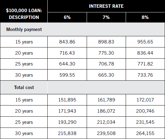
Every long-term mortgage balance drops on a predictable schedule. The longer the term, the more interest expense is involved; and the shorter the loan period, the higher the monthly payment. For example, compare the repayment terms and total costs for various interest rates and loan terms as shown in Table 3.3.

The shorter term saves significantly on total mortgage costs at each rate; however, as a practical matter, you will also need to be able to both afford the payment level and qualify with the lender. Terms for investors are often stricter than those for homeowners. For example, an investor is often required to make a larger down payment than a homeowner, and the investor may also need to meet stricter qualifying standards. Lenders compare monthly estimated cash flow to existing income and expense levels. They may subtract an assumed vacancy factor from estimated income to reflect cash flow in the most conservative manner possible. So you first have to find out if you can qualify with a lender before deciding how (or whether) to pay off a mortgage more rapidly

Table 3.3: Loan Amortization Cost Comparisons

Investors need to not only find and qualify for the best possible loan but also to be able to calculate the monthly breakdowns between principal and interest. Some lenders provide this breakdown for you, but many do not. In order to properly record your mortgage payment in your books each month, you will need to be able to divide the payment between its two major components.

If your payment includes additional impound items (insurance and taxes), these have to be isolated before you perform the loan amortization calculation. So a payment may include two segments: principal/interest and impounds.

•Formula: Monthly Loan Amortization

P – {T [P * ( i ÷ 12)]} = N

where:

P	= previous balance, mortgage loan
T	= total payment
i	= interest rate
N	= new balance, mortgage loan

•Excel Program: Monthly Loan Amortization

= SUM(P-(T-(P*(i/12))))

where:

P	= previous balance, mortgage loan
T	= total payment
i	= interest rate

When this single-line formula is applied to the example ($100,000 loan, $599.55 monthly payment, and 6 percent annual interest), the formula is:

= SUM(100000-(599.55-(100000*(0.06/12))))

And the new balance forward is $99,900.45.

This can be broken down into a series of steps:

1.Calculate monthly interest for 6 percent per year:

.06 ÷ 12 = .005

2.Calculate interest for the current month:

.005 * $100,000 = $500.00

3.Deduct current interest from the total payment to arrive at principal amount:

$599.55 = $500.00 = $99.55

4.Deduct principal from the balance forward to discover the new balance forward:

$100,000 – $99.55 = $99,900.45

The Excel formula can be carried forward with the new balance as a starting point:

= SUM(99900.45-(599.55-(99900.45*(0.06/12))))

And the new balance forward is $99,800.40.

The same procedure is duplicated each month, as shown in Table 3.4.

Table 3.4: Mortgage Amortization, One Year

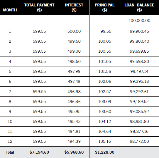
If you continue to calculate a year’s payments by hand, two important math checks should be performed. First is the verification between interest and principal. The sum of the two should equal the total of payments; if it does not, there is a math error in the calculations.

•Formula: Math Check, Interest/Principal

P + I = T

where:

P	= principal amount
I	= interest amount
T	= total of payments

•Excel Program: Math Check, Interest/Principal

A1:	principal amount
B1:	interest amount
C1:	= SUM(A1+B1)

The second verification step is to subtract the ending loan balance from the beginning loan balance; the net should be equal to the total principal for the year.

•Formula: Math Check, Change in Loan Balance

PB – NB = P

where:

PB	= previous balance
NB	= new balance
P	= principal payments

•Excel Program: Math Check, Change in Loan Balance

A1:	previous balance
B1:	new balance
C1:	= SUM(A1-B1)

CASH FLOW CALCULATIONS

The key to deciding whether a real estate investment is sensible is found in cash flow analysis. There are complex models of this analysis, as well as practical and easier ways to make comparative judgments.

One method is called discounted cash flow analysis. This is an estimate of the present value of future earnings, meaning what today’s cash flow is worth in terms of future profits. The problem with this model is that it is based on two models: one for today’s present value and the other for assumed earnings into the future. For most individual investors, discounted cash flow is too obscure to be of practical use.

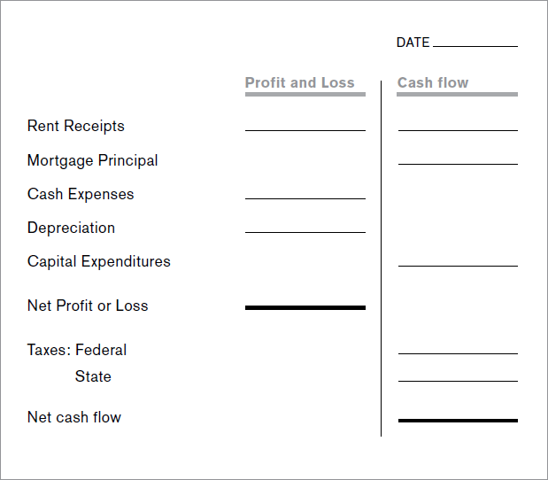
A far more immediate concern is the net cash flow you gain from real estate investments. This has to include calculation of tax benefits for reported losses because those benefits can be substantial. The actual calculation of cash flow requires certain adjustments, because cash flow is not simply a matter of figuring out rent income and expenses. The following items have to be adjusted:

1.Mortgage principal payments. The amount of interest paid each month is an expense, but the principal payments are not. So the portion of payments going to principal do not affect profits, but they do affect cash flow.

2.Depreciation expense. Cash expenses affect both profit and cash flow. However, one of the most significant expenses is depreciation, which is calculated based on the value of improvements (such as buildings, for example). While no cash is paid out for depreciation, a deduction is allowed. So depreciation (see Chapter 11) affects profits but not cash flow.

3.Capital expenditures. Any money spent for capital improvements to property, such as major repairs, equipment, and other depreciable assets, (see Chapter 8) affects cash flow, but those expenditures cannot be deducted as expenses.

4.Effect of reduced income taxes. If you report a loss on your tax return, your tax liability is reduced. This improves cash flow, so the benefit has to be calculated as part of your after-tax cash flows.

The combined effect of these adjustments is shown in the worksheet in Figure 3.1.

TAX EQUATIONS

To calculate each side (profit or loss and cash flow), each of the line items is treated differently.

•Formula: After-Tax Cash Flow

[R – (E + D)] – [P + C – T] = CF

where:

R	= rental income
E	= cash expenses
D	= depreciation
P	= principal payments
C	= capital expenditures
T	= income tax savings
CF	= after-tax cash flow

Figure 3.1: Worksheet, After-Tax Cash Flow

•Excel Program: After-Tax Cash Flow

A1:	rental income
B1:	cash expenses
C1:	depreciation
D1:	principal payments
E1:	capital expenditures
F1:	income tax savings
G1:	= SUM(A1-(B1+C1)-(D1+E1-F1)

In this calculation, the reported net loss is used to calculate the reduction in federal and state income taxes. This is based on your effective tax rate, which is the rate you pay in taxes based on your taxable income. In addition to the federal rate, you also need to calculate your effective tax rate for state-level income taxes.

To figure the federal and state tax benefit from reported real estate losses, multiply the loss by the effective tax rate; the result is the dollar amount of reduced taxes you gain from reporting the real estate loss.

•Formula: Tax Benefits from Reporting Losses

E * L = S

where:

E	= effective tax rate
L	= net loss from real estate
S	= savings from reduced taxes

•Excel Program: Tax Benefits from Reporting Losses

A1:	effective tax rate
B1:	net loss from real estate
C1:	= SUM(A1*B1)

The computation of mortgage breakdowns and the true cost of buying property affect cash flow directly. The time value of money—or, more accurately, the time expense of money—is perhaps the most important factor to consider when estimating profit and loss. Chapter 4 expands on this idea by exploring a series of specific investment calculations for real estate investors.