Chapter 8. Fractals
To understand fractals, we have to start with dimensions. The dimension of a space is the number of coordinates we need to specify a point in a space. A number line takes one coordinate, a Euclidean plane takes two, a solid takes three, and so on. See http://en.wikipedia.org/wiki/Dimension.
For simple geometric objects, dimension is defined in terms of
scaling behavior; that is, how size depends on length,
l. For example, the area of a square is
![]() ; the exponent, 2, indicates that a square is
two-dimensional. Similarly, the volume of a cube is
; the exponent, 2, indicates that a square is
two-dimensional. Similarly, the volume of a cube is ![]() , and a cube is three-dimensional. A line has dimension
1, and if we think of a point as infinitesimally small, it has dimension
0.
, and a cube is three-dimensional. A line has dimension
1, and if we think of a point as infinitesimally small, it has dimension
0.
Fractal dimension is a more precise and more general extension of this definition. There are several versions; the one I find easiest to understand and apply is the box-counting dimension, which is defined for a set, S, of points in a d-dimensional space. See http://en.wikipedia.org/wiki/Box-counting_dimension.
To compute the box-counting dimension, we divide the space into a
grid where the size of each cell is ![]() . Then we count
. Then we count ![]() , the number of cells that contain at
least one element of S. As
, the number of cells that contain at
least one element of S. As ![]() gets smaller,
gets smaller, ![]() gets bigger. For many objects the
relationship has the following form:
gets bigger. For many objects the
relationship has the following form:
The box-counting dimension, ![]() , is defined to be the exponent,
D. Taking the log of both sides and rearranging
yields:
, is defined to be the exponent,
D. Taking the log of both sides and rearranging
yields:
More formally, ![]() is the limit of this ratio as
is the limit of this ratio as ![]() goes to zero.
goes to zero.
Fractal CAs
To investigate the behavior of the fractal dimension, we’ll apply it to cellular automata. Box counting for CAs is simple; we just count the number of “on” cells in each time step and add them up.
As an example, consider Rule 254. Figure 8-1
shows what it looks like after ![]() time steps, and Figure 8-2
shows what it looks like after
time steps, and Figure 8-2
shows what it looks like after ![]() time steps.
time steps.
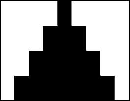
As t increases, we can imagine the triangle
getting bigger, but for purposes of box counting, it makes more sense to
imagine the cells getting smaller. In that case, the size of the cells,
![]() , is just
, is just ![]() .
.
After one time step, there is one black cell. After 2 time steps,
there are a total of 4, then 9, then 16, then 25. As expected, the area
of the triangle goes up quadratically. More formally,
![]() , so
, so ![]() . We conclude that a triangle is
two-dimensional.
. We conclude that a triangle is
two-dimensional.
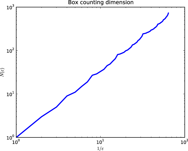
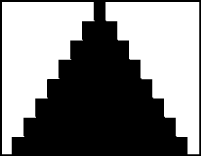
Rule 18 is more interesting. Figure 8-3 shows
what it looks like after 64 steps, and Figure 8-4
shows ![]() versus
versus ![]() on a log-log scale.
on a log-log scale.
To estimate ![]() , I fit a line to this curve; its slope is 1.56.
, I fit a line to this curve; its slope is 1.56.
![]() is a non-integer, which means that this set of
points is a fractal. As
t increases, the slope approaches
is a non-integer, which means that this set of
points is a fractal. As
t increases, the slope approaches
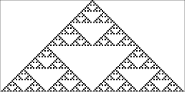
![]() , which is the fractal dimension of
Sierpiński’s triangle. See http://en.wikipedia.org/wiki/Sierpinski_triangle.
, which is the fractal dimension of
Sierpiński’s triangle. See http://en.wikipedia.org/wiki/Sierpinski_triangle.
Write a function that takes a CA object; plots
![]() versus
versus ![]() , where
, where ![]() ; and estimates
; and estimates ![]() .
.
Can you find other CAs with non-integer fractal dimensions? Be
careful, you might have to run the CA for a while before
![]() converges.
converges.
Here are some functions from numpy you might find useful: cumsum, log, and polyfit.
You can download my solution from http://thinkcomplex.com/fractal.py.
In 1990, Bak, Chen, and Tang proposed a cellular automaton that is an abstract model of a forest fire. Each cell is in one of three states: empty, occupied by a tree, or on fire.
The rules of the CA are the following:
An empty cell becomes occupied with probability p.
A cell with a tree burns if any of its neighbors is on fire.
A cell with a tree spontaneously burns with probability f, even if none of its neighbors is on fire.
A cell with a burning tree becomes an empty cell in the next time step.
Read about this model at http://en.wikipedia.org/wiki/Forest-fire_model, and write a program that implements it. You might want to start with a copy of http://thinkcomplex.com/Life.py.
Starting from a random initial condition, run the CA until it reaches a steady state where the number of trees no longer increases or decreases consistently. You might have to tune p and f.
In a steady state, is the geometry of the forest fractal? What is its fractal dimension?
Percolation
Many of the CAs we have seen so far are not physical models; that is, they are not intended to describe systems in the real world. But some CAs are designed explicitly as physical models. In this section, we consider a simple grid-based model of percolation; in the next chapter, we see examples that model forest fires, avalanches, and earthquakes.
Percolation is a process in which a fluid flows through a semiporous material. Examples include oil in rock formations, water in paper, and hydrogen gas in micropores. Percolation models are also used to study systems that are not literally percolation, including epidemics and networks of electrical resistors; see http://en.wikipedia.org/wiki/Percolation_theory.
Percolation processes often exhibit a phase change; that is, an abrupt transition from one behavior (low flow) to another (high flow) with a small change in a continuous parameter (like the porosity of the material). This transition is sometimes called a “tipping point.”
There are two common models of these systems: bond percolation and site percolation. Bond percolation is based on a grid of sites where each site is connected to four neighbors by a bond. Each bond is either porous or non-porous. A set of sites that are connected (directly or indirectly) by porous bonds is called a cluster. In the vocabulary of graphs, a site is a vertex, a bond is an edge, and a cluster is a connected subgraph.
Site percolation is based on a grid of cells where each cell represents a porous segment of the material or a non-porous segment. If two porous cells are adjacent, they are considered connected; a set of connected cells is considered a cluster.
The rate of flow in a percolation system is primarily determined by whether or not the porous cells form a path all the way through the material, so it is useful to know whether a set of cells (or bonds) contains a “spanning cluster.” There are several definitions of a spanning cluster; the choice depends on the system you are trying to model. The simplest choice is a cluster that reaches the top and bottom row of the grid.
To model the porosity of the material, it is common to define a
parameter, p, of the probability that any cell (or
bond) is porous. For a given value of p, you can
estimate ![]() —which is the probability that there
is a spanning cluster—by generating a large number of random grids and
computing the fraction that contain a spanning cluster. This way of
estimating probabilities is called a Monte Carlo simulation because it a
similar to a game of chance.
—which is the probability that there
is a spanning cluster—by generating a large number of random grids and
computing the fraction that contain a spanning cluster. This way of
estimating probabilities is called a Monte Carlo simulation because it a
similar to a game of chance.
Percolation models are often used to compute a critical value, pc, which is the fraction of porous segments where the phase change occurs; that is, where the probability of a spanning cluster increases quickly from near 0 to near 1.
The paper “Efficient Monte Carlo Algorithm and High-Precision Results for Percolation,” by Newman and Ziff, presents an efficient algorithm for checking whether there is a path through a grid. You can download this paper from http://arxiv.org/abs/cond-mat/0005264. Read the paper, implement their algorithm, and see if you can reproduce their Figure 2(a).
What is the difference between what Newman and Ziff call the “microcanonical ensemble” and the “canonical ensemble”? You might find it useful to read about the use of these terms in statistical mechanics at http://en.wikipedia.org/wiki/Statistical_mechanics. Which one is easier to estimate by Monte Carlo simulation?
What algorithm do they use to merge two clusters efficiently?
What is the primary reason their algorithm is faster than the simpler alternative?