
This chapter is a brief review of IPv4,1 the foundation protocol of the Second Internet. I am covering it in this chapter to help you understand what is new and different in IPv6. It is not intended to be comprehensive. There are many great books listed in the bibliography if you wish to understand IPv4 at a deeper level. The reason IPv4 is relevant in this book is because the design of IPv6 is based heavily on that of IPv4. First, IPv4 can be considered one of the great achievements in IT history, based on its worldwide success, so it was a good model to copy from. Second, there were several attempts to do a new design “from the ground up” with IPv6 (a “complete rewrite”). These involved really painful migration and interoperability issues. You need to understand what the strengths and weaknesses of IPv4 are to see why IPv6 evolved the way it did. You can think of IPv6 as “IPv4 on steroids,” which takes into account the radical differences in the way we do networking today and fixing problems that were encountered in the first three decades of the IP-based Internet, as network bandwidth and the number of nodes increased exponentially. We are doing things over networks today that no one could have foreseen a quarter of a century ago, no matter how visionary they were.
Network Hardware
There are many types of hardware devices used to construct an Ethernet network running TCP/IP. These include nodes, Network Interface Cards (NICs), cables, hubs, switches, routers, and firewalls.
A node is a device (usually a computer) that can do processing and has some kind of wired or wireless connection(s) to a network. Examples of nodes are desktop computers, notebook computers, netbooks, smartphones, hubs,2 switches,3 routers,4 wireless access points,5 network printers, network-aware appliances, and so on. A node could be as simple as a temperature sensor, with no display and no keyboard, just a connection to a network. It could have a display and keyboard or be a “headless node” with a management interface accessed via the network with Telnet, Secure Shell 6 (SSH), or a web browser. All nodes connected to a TCP/IP network must have at least one valid IP address 7 (per interface). If a node has only one network interface, such as a workstation computer, it is called a host. If a node has multiple interfaces connected to different networks, and the ability to forward packets between them, it is called a gateway or a router. Routers and firewalls are special types of gateways that can forward packets between networks and/or control traffic in various ways as it is forwarded. Gateways make it possible to build internetworks .8 They are described in more detail under the “IPv4 Routing” section in this chapter.
A NIC 9 (or Network Interface Controller ) is the physical interface that connects a node to a network. It may also be called an Ethernet adapter if the network is based on Ethernet. It should have a female RJ-4510 connector on it (or possibly a coax or fiber-optic connector). It could be an actual add-in Peripheral Computer Interconnect (PCI 11) card. It could be integrated on the device’s motherboard. It could also be something that makes a wireless connection to a network, using Wi-Fi, WiMAX, or similar standard. Typically, all NICs have a globally unique, hard-wired MAC address 12 (48 bits long, assigned by the manufacturer). A node can have one or more NICs (also called interfaces). Each interface can be assigned one or more IP addresses and various other relevant network configuration items, such as the address of the default gateway and the addresses of the DNS servers.
Network cables today are typically unshielded twisted pair 13 (UTP) cables that actually have four pairs of plastic-coated wires, with each pair forming a twisted coil. They have RJ-45 male connectors on each end. They could also be fiber-optic cables for very high-speed or long-run connections. Often today, professional contractors install UTP cables through the walls and bring them together at a central location (sometimes called the wiring closet) where they are connected together with a hub or a switch to form a star network.14 Cables typically are limited to 100 meters or less in length, but the maximum acceptable length is a factor of several things, such as network speed and cable design. Modern cables rated as “CAT5”15 or “CAT5E” are good up to 100 Mbps, while cables rated as “CAT6”16 are good up to a gigabit per second (1 Gbps). Today, you can get CAT7 cables for speeds up to 10 Gbps. Above that speed, you should be using optical fiber 17 NICs and cables. It is also possible for twisted pair cables to be shielded if required to prevent interference from (or with) other devices.
An Ethernet hub 18 is a device that connects multiple Ethernet cables together so that any packet transmitted by any node connected to that hub is relayed to all the other nodes connected to the hub. It typically has a bunch of female RJ-45 connectors in parallel (called ports). In effect it ties together the network cables plugged into it into a star network. Hubs have a speed rating, based on what speed Ethernet they support. Older hubs might be only 10 Mbps. More recent ones might be “fast Ethernet,” which means they support 100 Mbps. If you have five nodes (A, B, C, D, and E) connected together with a hub and node B sends a packet to node D, all nodes, including A, C, and E, will see the traffic. The nodes not involved in the transaction will typically just discard the traffic. This dropping of packets not addressed to a node is often done by the hardware in the NIC, so that it never interrupts the software driver. Many NICs have the ability to be configured in promiscuous mode .19 When in this mode, they will accept packets (and make them available to any network application) whether those packets are addressed to this node or not. If this mode is selected, the dropping of packets not addressed to you must be done in software. However, sometimes you want to see all traffic on the subnet. For instance, this would be useful with intrusion detection, for diagnostic troubleshooting, or for collecting network statistics. Hubs come in various sizes, from 4 ports up to 48 ports, and can even be coupled with other hubs to make large network “backbones.” You can also have a hierarchy of hubs, where several hubs distributed around a company actually connect into a larger (and typically faster) central hub. Hubs do no processing of the packets; they are really just a cluster of Ethernet extenders 20 (repeaters) that clean up and relay any incoming signals from any port to all the other ports. Hubs are quite rare today. Most such devices today are now actually switches.
A network switch 21 is similar to a network hub but has some control logic that minimizes unnecessary traffic. It partitions a LAN into multiple collision domains 22 (one per switch port). Again, say you have a switch with cables connected to nodes A, B, C, D, and E. If B sends a packet to D, that packet will be sent out only to the port to which D is connected. Switches learn what nodes are connected to what ports by maintaining a table of MAC addresses vs. port number. When a switch is first powered on, this table is empty. As the nodes send packets through the switch, it learns what port each node is connected to.
If node A (connected to port 1) sends a packet to node B (connected to port 2), the switch adds the MAC address of A and the port it was seen on (1) to its table. In the future, when packets for A’s MAC address come in any port, they will only be sent out port 1. Since the switch hasn’t previously seen the MAC address of B (as a source address), it doesn’t know where B is located, so it sends this first packet out to all ports. If B replies to A’s packet, the switch adds B’s MAC address and port (2) to the table. In the future, packets sent to B’s MAC address will only be sent out port 2. Each addition to the table expires after a certain amount of time, to allow nodes to be moved to other ports. An incoming packet sent to a broadcast address will always be sent out to all ports. This behavior holds down excessive traffic that would normally just be dropped anyway by the unaddressed nodes (not to mention unnecessary packet collisions). It also provides a small degree of privacy, even if someone enables their NIC in promiscuous mode. If your LAN is built using switches instead of hubs, you can typically only sniff traffic originating from or terminating on the network segment connected to your port of the switch. Most switches are oblivious to IP addresses – they work only with MAC addresses. Because of this, they are IP version agnostic. This means they will carry IPv4 or IPv6 traffic (or even other kinds of Ethernet traffic) so long as that traffic uses Ethernet frames with MAC addresses.
If you are using a switch, but one of your connected nodes really does want to see traffic from other network segments, some switches have a mirror port function that will allow all traffic from any combination of ports to be copied to one port, to which you connect the node that wants to monitor that traffic. This must be configured, which requires a management interface of some kind. Like hubs, switches come in various speeds, from 10 Mbps up to 1000 Mbps (1 Gbps). Unlike hubs, you can mix different speed nodes (10 Mbps, 100 Mbps, and even 1000 Mbps) on a single switch, so the speed rating is the maximum speed for nodes connected to it. Switches also come in sizes from 4 ports up to 48 ports, and better ones can be “stacked” (linked together) to effectively build a single giant switch. Lower-end (cheaper) switches may have few if any configuration options and may not even have a user interface. Smart (or managed) switches typically have a sophisticated GUI management interface (accessible via the network, usually over HTTP) or Command Line Interface (accessible either via a serial port, Telnet, or SSH) that allows you to configure various things and/or monitor traffic. Switches also typically include support for monitoring or control using SNMP (Simple Network Monitoring Protocol). Very advanced switches allow you to configure VLANs (Virtual Local Area Networks 23), which allow you to effectively create multiple sub-switches that are not logically connected together, on a single physical switch. Some of these advanced functions process IP addresses (layer 3 functionality) and hence are IP version specific (an IPv4-only smart switch cannot process IPv6 addresses, but the basic layer 2 switch functionality may work fine). Very recent smart switches do support both IPv4 and IPv6 (dual stack), for layer 3 functionality with both IP versions.
RFCs: The Internet Standards Process
Anyone studying the Internet, or developing applications for it, must understand the RFC 24 system. RFC stands for Request for Comments . These are the documents that define the Internet Protocol Suite (the official name for TCP/IP) and many related topics. Anyone can submit an RFC. Ones that are part of the Standards Track are usually produced by the IETF (Internet Engineering Task Force ) working groups. Anyone can start or participate in a working group. Submitted RFCs begin life as a series of Internet Drafts, each of which has a lifespan of 6 months or less. Most drafts go through considerable peer review, and possibly quite a few revisions, before they are either abandoned or approved and issued an official RFC number (e.g., 793) and become part of the official RFC collection. There are other kinds of documents in addition to the Standards Track, including information memos (FYI), humor (primarily ones issued on April 1), and even one obituary, for Jon Postel, the first RFC editor and initial allocator of IP addresses, RFC 2468,25 “I Remember IANA,” October 1998. There is even an RFC about RFCs, RFC 2026,26 “The Internet Standards Process, Revision 3,” October 1996. That is a good place to start if you really want to learn how to read RFCs.
The Internet Standards Process is quite different from the standards process of the ISO (International Organization for Standardization) that created the Open System Interconnection (OSI) network specification. The ISO typically develops large, complex standards with multiple four-year cycles, with hundreds of engineers and much political wrangling. This was adequate for creating the standards for the worldwide telephony system but is far too slow and hidebound for something as freewheeling and rapidly evolving as the Internet. The unique standards process of the IETF is one of the main reasons that TCP/IP is now the dominant networking standard worldwide. By the time OSI was specified, TCP/IP was already created, deployed, and being revised and expanded. OSI never knew what hit it.
Learning to read RFCs is an acquired skill, one that anyone serious about understanding the Internet, and most developers creating things for it, should master. There are certain “terms of art” (terms that have precise and very specific meanings), like the usage of MUST, SHOULD, MAY, and NOT RECOMMENDED. As an example, the IPv6-ready tests examine all the MUST (mandatory) and SHOULD (optional) items from relevant RFCs.
www.rfc-editor.org/rfc/rfcXXXX.txt (where XXXX is the RFC number)
There are over 8000 RFCs today. I have included many references to the relevant RFCs in this book. If you want to see all the gory details on any subject, go right to the source and read it. You may find it somewhat tough going until you learn to read “RFC-ese.” A number of books on Internet technology are either just a collection of RFCs, or RFCs make up a large part of the content. There is no reason today to do that – anyone can download all the RFCs you want and have them in soft (searchable) form. I have not included the text of even a single RFC in this book (warning: if you try to read this book somewhere without Internet access like on a plane, you may want to look ahead and download any relevant RFCs while you have Internet access). The casual reader should not need to reference the actual RFCs. The complete set of RFCs is easily tens of thousands of pages and growing daily.
Most of the topics covered in this book also have considerable coverage on the Internet outside of the RFCs, such as in Wikipedia. Again, if you want to drill deeper in any of these topics, crank up your favorite search engine and have at it. The information is out there. What I’ve done is to try to collect together the essential information in a logical sequence, with a lot of explanations and examples, plus all the references you need to drill as deep as you like. I taught cryptography and Public Key Infrastructure for VeriSign for two years, so I have a lot of experience trying to explain complex technical concepts in ways that reasonably intelligent people can easily follow. Hopefully you will find my efforts worthwhile.
IPv4
The software that made the Second Internet (and virtually all Local Area Networks) possible has actually been around for quite some time. It is technically a suite (family) of protocols. The core protocols of this suite are TCP (the Transmission Control Protocol) and IP (Internet Protocol), which gave it its common name, TCP/IP. Its official name is the Internet Protocol Suite.
TCP was first defined officially in RFC 675, “Specification of Internet Transmission Control Program,” December 1974 (yes, 45 years ago). The protocol described in this document does not look much like the current TCP, and in fact, the Internet Protocol (IP) did not even exist at the time. Jon Postel was responsible for splitting the functionality described in RFC 675 into two separate protocols: (the new) TCP and IP . RFC 675 is largely of historical interest now. The modern version of TCP was defined in RFC 795, “Transmission Control Protocol – DARPA Internet Program Protocol Specification,” September 1981 (7 years later). It was later updated by RFC 1122, “Requirements for Internet Hosts – Communication Layers,” October 1989, which covers the Link Layer, IP Layer, and Transport Layer. It was also updated by RFC 3168, “The Addition of Explicit Congestion Notification (ECN) to IP,” September 2001, which adds ECN to TCP and IP.
Both of these core protocols, and many others, will be covered in considerable detail in the rest of this chapter.
Four-Layer (“DoD”) IPv4 Architectural Model

A four-layer D o D model for I P V 4 has, from top to bottom, the application layer, transport layer, internet layer v 4, and the link layer.
Four-layer DoD model for IPv4

An illustrated block diagram depicts how the data flows through the four layers of the D o D model. It contains a source, an I P packet, and a destination. Arrows mark the data flow direction.
Data flow in the four-layer model
It just confuses the issue to try to figure out which of the seven OSI layers the various protocols of TCP/IP fit into. It is simply not applicable. It’s like trying to figure out what color “sweet” is. The OSI seven-layer model did not even exist when TCP/IP was defined. Unfortunately, many people use terms like “layer 2” switches vs. “layer 3” switches. These refer to the OSI model. Books from Cisco Press and the Cisco certification exams are particularly adamant about using OSI terminology. I would be surprised if there is even a single actual OSI network running today. In this book we will try to consistently use the four-layer model terminology while referring to the OSI terminology when necessary for you to relate the topic to actual products or other books.
Note: Outgoing data begins in the application and is passed down the layers of the stack (adding headers at each layer) until it is written to the wire. Incoming data is read off the wire and travels up the layers of the stack (processing and removing headers at each layer) until it is accepted by the application. In the following discussion, for simplicity, I describe only the outgoing direction.
The Application Layer 27 implements the protocols most people are familiar with (e.g., HTTP, SMTP, FTP). The software routines for these are typically contained in application programs such as browsers or web servers that make “system calls” to subroutines (or “functions” in C terminology) in the “socket API”28 (an API is an Application Program Interface, or a collection of related subroutines, typically supplied with the operating system or C programming language compiler). The application code creates outgoing data streams and then calls routines in the socket API to actually send the data via TCP (Transmission Control Protocol) or UDP (User Datagram Protocol). Output to the Transport Layer is [DATA] using IP addresses.
The Transport Layer 29 implements TCP 30 (the Transmission Control Protocol) and UDP 31 (the User Datagram Protocol). These routines are internal to the socket API (hence live in Kernel Space 32). In the case of TCP, packet sequencing, plus error detection and retransmission, is handled. The Transport Layer prepends a TCP or UDP packet header to the data passed down from the Application Layer and then passes the resulting packet down to the Internet Layer for further processing. Output to the Internet Layer is [TCP HDR[DATA]], using IP addresses.
The Internet Layer 33 implements IP 34 (the Internet Protocol) and various other related protocols such as ICMP 35 (which includes the “ping” function among other things). The IP routine takes the data passed down from the Transport Layer routines, adds an IP packet header onto it, and then passes the now complete IPv4 packet down to routines in the Link Layer. Output to the Link Layer is [IP HDR[TCP HDR[DATA]]] using IP addresses.
The Link Layer 36 implements protocols such as ARP 37 (Address Resolution Protocol ) that map IP addresses to MAC addresses for transmission between nodes in a single network link. It contains protocols such as Ethernet, Wi-Fi, and MPLS. It also contains routines that actually read and write data (as fed down to it by routines in the Internet Layer) onto the network wire, in compliance with Ethernet or other standards. Output to wire: Ethernet frame containing the IP packet, using MAC addresses (or other Link Layer addresses for non-Ethernet networks).
Each layer “hides” the details (and/or hardware dependencies) from the higher layers. This is called “levels of abstraction.” An architect thinks in terms of abstractions such as roofs, walls, windows, etc. The next layer down (the builder) thinks in terms of abstractions such as bricks, glass, mortar, etc. Below the level of the builder, an industrial chemist thinks in terms of formulations of clay or silicon dioxide to create bricks and glass. If the architect tried to think at the chemical or atomic level, it would be very difficult to design a house. Their job is made possible by using levels of abstraction. Network programming is analogous. If application programmers had to think in terms of writing bits to the actual hardware, applications such as web browsers would be almost impossible. Each Network Layer is created by specialists who understand the details at their level, and lower layers can be treated as “black boxes” by people working at the higher layers.
Another important thing about Network Layers is that you can make major changes to one layer, without impacting the other layers much at all. The connections between layers are well defined and don’t change (much). This provides a great deal of separation between the layers. In the case of IPv6, the Internet Layer is almost completely redesigned internally, while the Link Layer and Transport Layer are not affected much at all (other than providing more bytes to store the larger IPv6 addresses). If your product is “IPv6-only,” that’s about the only change you would need to make to your application software (unless you display or allow entry of IP addresses). If your application is “dual stack” (can send and receive data over IPv4 or IPv6), then a few more changes are required in the Application Layer (e.g., to accept multiple IPv4 and IPv6 addresses from DNS and try connecting to one or more of them based on various factors or to accept incoming connections over both IPv4 and IPv6). This makes it possible to migrate (or “port”) network software (created for IPv4) to IPv6 or even dual stack with a fairly minor effort. In comparison, changing network code written for TCP/IP to use OSI instead would probably involve a complete redesign and major recoding effort.
IPv4: The Internet Protocol, Version 4
IPv4 is the foundation protocol of the Second Internet and accounts for many of its distinguishing characteristics, such as its 32-bit address size, its addressing model, and its packet header structure and routing. IPv4 was first defined in RFC 791 “Internet Protocol,” September 1981.
Relevant Standards for IPv4
RFC 791 , “Internet Protocol,” September 1981 ( Standards Track )
RFC 792 , “Internet Control Message Protocol,” September 1981 (Standards Track)
RFC 826 , “An Ethernet Address Resolution Protocol,” November 1982 (Standards Track)
RFC 1256, “ICMP Router Discovery Messages,” September 1991 (Standards Track)
RFC 2390, “Inverse Address Resolution Protocol,” September 1998 (Standards Track)
RFC 2474 , “Definition of the Differentiated Services Field (DS Field) in the IPv4 and IPv6 Headers,” December 1998 (Standards Track)
RFC 4650, “HMAC-Authenticated Diffie-Hellman for Multimedia Internet KEYing (MIKEY),” September 2006 (Standards Track)
RFC 4884, “Extended ICMP to Support Multi-Part Messages,” April 2007 (Standards Track)
RFC 4950, “ICMP Extensions for Multiprotocol Label Switching,” August 2007 (Standards Track)
RFC 5494, “IANA Allocation Guidelines for the Address Resolution Protocol (ARP),” April 1009 (Standards Track)
RFC 5735 , “Special Use IPv4 Addresses,” January 2010 (Best Current Practices)
IPv4 Packet Header Structure

An illustration depicts the I P v 4 packet header. The packet consists of 7 layers. The first part of the packet is the I P version, and the last part consists of the data.
IPv4 packet header
The IP Version field (4 bits) contains the value 4, which in binary is “0100” (you’ll never guess what goes in the first 4 bits of an IPv6 packet header!).
The Header Length field (4 bits) indicates how long the header is, in 32-bit “words.” The minimum value is “5,” which would be 160 bits, or 20 bytes. The maximum length is 15, which would be 480 bits, or 60 bytes. If you skip that number of words from the start of the packet, that is where the data starts (this is called the “offset” to the data). This will only ever be greater than 5 if there are options before the data part (which is not common).
The Type of Service field (8 bits) is defined in RFC 2474,39 “Definition of the Differentiated Services Field (DS Field) in the IPv4 and IPv6 headers,” December 1998. This is used to implement a fairly simple QoS (Quality of Service ). QoS involves management of bandwidth by protocol, by sender, or by recipient. For example, you might want to give your VoIP connections a higher priority than your video downloads or the traffic from your boss higher priority than your co-worker’s traffic. Without QoS, bandwidth is on a first come–first served basis. 8 bits are not really enough to do a good job on QoS, and DiffServ is not widely implemented in current IPv4 networks. QoS is greatly improved in IPv6.
The Total Length field (16 bits) contains the total length of the packet (including the packet header) in bytes. The minimum length is 20 (20 bytes of header plus 0 bytes of data), and the maximum is 65,535 bytes (since only 16 bits are available to specify this). All network systems must handle packets of at least 576 bytes, but a more typical packet size is 1508 bytes. With IPv4, it is possible for some devices (like routers) to fragment packets 40 (break them apart into multiple smaller packets) if required to get them through a part of the network that can’t handle packets that big. Packets that are fragmented must be reassembled at the other end. Fragmentation and reassembly is one of the messy parts of IPv4 that got cleaned up a lot in IPv6. A lot of hacking attacks exploit the messy scheme in IPv4.
The Identification (Fragment ID) field (16 bits) identifies which fragment of a once larger packet this one is, to help in reassembling the fragmented packet later. In IPv6 packet fragmentation is not done by intermediate nodes, so all the header fields related to fragmentation are no longer needed.
The next three bits are flags related to fragmentation. The first is reserved and must be zero (an April Fool’s RFC 41 once defined this as the “evil” bit, which the sender should set if they are doing something malicious). The next bit is the DF (Don’t Fragment) flag. If DF is set, the packet cannot be fragmented (so if such a packet reaches a part of the network that can’t handle one that big, that packet is dropped). The third bit is the MF (More Fragments) flag. If MF is set, there are more fragments to come. Unfragmented packets of course have the MF flag set to zero.
The Fragment Offset field (13 bits) is used in reassembly of fragmented packets. It is measured in 8-byte blocks. The first fragment of a set has an offset of 0. If you had a 2500-byte packet, and were fragmenting it into chunks of 1020 bytes, you would have three fragments as follows:

A table with five columns and four rows. The column headers are fragment I D, M F flag, total length, data size, and offset.
The Time-To-Live (TTL) field (8 bits) is to prevent packets from being shuttled around indefinitely on a network. It was originally intended to be lifetime in seconds (hence the name), but it has come to be implemented as “hop count.” This means that every time a packet crosses a switch or router, the hop count is decremented by one. If that count reaches zero, the packet is dropped. Typically, if this happens, an ICMPv4 message (“Time Exceeded”) is returned to the packet sender. This mechanism is how the traceroute command works. The primary purpose of TTL is to prevent looping (packets running around in circles).
The Protocol field (8 bits) defines the type of data found in the data portion of the packet. Protocol numbers are not to be confused with ports. Some common protocol numbers are

A table with 7 rows and 3 columns contains protocol details. The first column has the protocol numbers, and the next has the protocol acronyms, followed by their corresponding abbreviations.
The Header Checksum field (16 bits) is the 16-bit one’s complement of the one’s complement sum of all 16-bit words in the header. When computing, the checksum field itself is taken as zero. To validate the checksum, add all 16-bit words in the header together including the transmitted checksum. The result should be 0. If you get any other value, then at least 1 bit in the packet was corrupted. There are certain multiple bit errors that can cancel out, and hence bad packets can go undetected. Note that since the hop count (TTL) is decremented by one on each hop, the IP header checksum must be recalculated at each hop. The IP header Checksum was eliminated in IPv6.
The Source IP Address field (32 bits) contains the IPv4 address of the sender (may be modified by NAT).
The Destination IP Address field (32 bits) contains the IPv4 address of the recipient (may be modified by NAT in a reply packet).
Options (0–40 bytes) is not often used. These are not relevant to this book. If you want the details, read the RFCs.

An illustration depicts the I P v 4 and I P v 6 packet headers side by side, showcasing their difference.
IPv4 and IPv6 packet headers side by side

A text box represents ten changes between the I P v 4 and I P v 6 headers.
IPv4 Addressing Model
In IPv4, addresses are 32 bits in length. They are really just integer numbers from 0 to 4,294,967,295. For the convenience of humans, these numbers are typically represented in dotted decimal notation . This splits the 32-bit addresses into four 8-bit fields and then represents each 8-bit field with a decimal number from 0 to 255. These decimal numbers cover all possible 8-bit binary patterns from 0000 0000 to 1111 1111. The decimal numbers are separated by “dots” (periods). Leading zeros can be eliminated. The following are all valid IPv4 addresses represented in dotted decimal:

Four I P v 4 addresses consist of a globally routable address, a private address, a broadcast address, and a loopback address.
Originally there were five classes of IPv4 addresses, as defined in RFC 791,42 “Internet Protocol,” September 1981:
Class A: First bit 0 (0.0.0.0–127.255.255.255), 8-bit network number, 24-bit node within network number, subnet mask 255.0.0.0. There are 128 class A networks, each containing 16.7M addresses.
Class B: First 2 bits “10” (128.0.0.0–191.255.255.255), 16-bit network number, 16-bit node within network number, subnet mask 255.255.0.0. There are 16,384 class B networks, each containing 65,536 addresses.
Class C: First 3 bits “110” (192.0.0.0–223.255.255.255), 24-bit network number, 8-bit node within network number, subnet mask 255.255.255.0. There are 2M class C networks, each containing 256 addresses.
Class D: First 4 bits “1110” (224.0.0.0–239.255.255.255), used for multicast.
Class E: First 4 bits “1111” (240.0.0.0–255.255.255.255), experimental/reserved (not forwarded by most routers).
Network Ports
Each IP address on a network node has 65,536 ports associated with it (the port number is a 16-bit value, and 2 to the 16th is 65,536). Any of those ports can either be used to make an outgoing connection or to accept incoming connections. There is a list of well-known ports 43 that associates particular ports with certain protocols. For example, port 25 is associated with SMTP. There is nothing magical (or email-ish) about port 25. SMTP will work just as well on any other port, for example, 10025. Use of port 25 for SMTP is simply a convention that many people adopt. Such conventions make it easier to locate the SMTP server on a node you might not be familiar with. To be specific, ports are a Transport Layer thing, and there are really 65,536 TCP ports and another 65,536 UDP ports for each address. IP and ICMP, which are Internet Layer things, do not have any port(s) associated with them.

A screenshot depicts a table containing the details of an I R P port number registration process. It has eight columns and two rows.
IRP port number registration
When you deploy an Internet server (e.g., an SMTP server for sending and receiving email), the software opens a socket (a programming abstraction) in listen mode on a particular port (in the case of SMTP, port 25). An email client that wants to connect to it creates its own socket in connect mode and tells it to connect to a particular IP address (that of the SMTP server) using a particular port (in this case 25). When the connection attempt reaches the server, the server detects the attempt and accepts the connection (actually the port on the server that the connection is accepted on will be any available port, typically higher than 1024). A well-written server would then make a clone of itself (this is called forking in UNIX speak) and then go back to listening for further connections, while its clone went ahead and processed the connection. When the processing is complete on a given connection, the sockets used would be closed (on both server and client), and the clone of the server will quietly commit suicide. In theory you could have thousands of clones of the server all simultaneously handling email connections on a single server (given sufficient memory and other resources). Busy web servers (like those at Google) often have many thousands of connections being processed at any given time (but never more than 65,000 on a given interface – each connection uses up one port).
If threads are used instead of processes, the scheme is similar but has far less overhead.
In UNIX, ports with numbers under 1024 are special, and only software that has root privilege can use them. Most common Internet services use ports in that range. There are many well-known ports , but here are a few of the more common ones:

An image displays eight port numbers, along with their acronyms and abbreviations.
IPv4 Subnetting
This leads us naturally into the topic of IPv4 subnetting.45 This is one of the more difficult areas of networking for people learning to work with IPv4. All addresses have two “parts,” the first part being the address of the network (e.g., 192.168.0.0) and the second being the node within that network (e.g., 0.0.2.5). These two parts can be split apart at some “bit boundary.” In this case, the address of the network is in the first 16 bits, and the node within the network is in the last 16 bits. The addresses of all nodes in such a network share the same first 16 bits, but each has a unique last 16 bits. So such a network might have nodes with addresses 192.168.2.5, 192.168.3.7, and 192.168.200.12, but not one with the address 192.169.2.1 (that address is in network 192.169.0.0, not network 192.168.0.0).

An illustration of an I P address using a subnet mask and without it. It presents the I P address in both decimal and binary forms.
IP addresses and subnet masks
For subnet mask 255.0.0.0 (class A), the first 8 bits are the network address, and the last 24 are the node within subnet.
For subnet mask 255.255.0.0 (class B), the first 16 bits are the network address, and the last 16 are the node within subnet.
For subnet mask 255.255.255.0 (class C), the first 24 bits are the network address, and the last 8 are the node within subnet.
Subnetting was easy when the three IP address classes (A, B, and C) were used. The first few bits of the address determined the subnet mask. If the first bit of the 32-bit address was “0,” then the address was class A, and the subnet mask was 255.0.0.0. If the first 2 bits of the address were “10,” then the address was class B, and the subnet mask was 255.255.0.0. If the first 3 bits of the address were “110,” then the address was class C, and the subnet mask was 255.255.255.0. This could actually be done automatically, so no one worried about subnet masks.
One of the changes made in the IPv4 addressing model in the mid-1990s was to introduce Classless Inter-domain Routing,47 in RFC 1519,48 “Classless Inter-domain Routing (CIDR),” September 1993. It was later replaced by RFC 4632 49, “Classless Inter-domain Routing (CIDR) ,” August 2006.
When CIDR was introduced, there were two consequences. First, the split between the two parts of the address could come at any bit boundary, not just after 8, 16, and 24 bits. Second, several small blocks (e.g., /28 blocks) could be carved out of a bigger block anywhere in the address space (perhaps from an old class A block, such as 7.x.x.x), so you could no longer determine the correct subnet mask by looking at the first few bits of an address. For example, a “/8” (class A) block might be carved up into 65,536 “/24” (class C) subnets, which could be allocated to different organizations.
Let’s say your ISP, instead of giving you a class C block, only gives you a “/28” block of real (routable) IPv4 addresses, which would be 16 real IPv4 addresses, for example, 123.45.67.0 through 123.45.67.15. First, two of these addresses are not usable (may not be assigned to nodes). 123.45.67.0 is the “network address,” and 123.45.67.15 is the “broadcast address.” That leaves 14 usable addresses (123.45.67.1 through 12.45.67.14). So what is your subnet mask? If you check the preceding table of useful CIDR block sizes, a /28 subnet has a subnet mask of 255.255.255.240. In binary that is 1111 1111 1111 1111 1111 1111 1111 0000 (first 28 bits are 1; last 4 bits are 0). However, by the old rules (first bit is a 0), these are really from a “class A” block, so the automatically generated subnet mask would have been 255.0.0.0, which is not correct.
Now, what if your organization really has 100 nodes that need IP addresses? How do you give each of them unique addresses if you only have 14 usable addresses to work with? That’s where Network Address Translation (NAT) comes in (covered in the next chapter). If you think CIDR made your life more “interesting,” wait until you see what NAT does to it! Getting rid of CIDR and NAT is one of the big wins in IPv6. In fact, you will find that the entire subject of subnets has become totally trivial.
MAC Addresses
IPv4 addresses are not actually used at the lowest layer of the IPv4 network stack (the Link Layer). Each network hardware interface actually has a 48-bit “MAC address ” burned into it by the manufacturer. The first 24 bits of this (called the “Organizationally Unique Identifier 50” or OUI) specify the manufacturer and are purchased by vendors from the IEEE 51 (Institute of Electrical and Electronics Engineers). A given vendor may have multiple OUIs, but a given OUI is associated only with one vendor. The last 24 bits of this (called the “Network Interface Controller–Specific” part) are assigned by each manufacturer, to be unique within a given OUI. This means that the entire 48-bit value is globally unique. For example, Dell Computer has a number of OUIs assigned to them by the IEEE, including 00-06-5B, 00-08-74, and 00-18-8B. If you encounter a NIC with a MAC address that has one of those sets of 24 bits, it was made by Dell Computer. When you use the command “ipconfig /all” in Windows, you get a list of network configuration information for all your interfaces (some of which are “virtual”). If you look for “Local Area Connection,” that is information about your main (or only) network connection to your LAN. Under that, you will see an item labeled “Physical Connection,” followed by six pairs of hex digits, separated by dashes. That is the MAC address of your Network Interface Controller (NIC) . Mine is 00-18-8B-78-DA-1A. This means my NIC was made by Dell (my whole computer was, but the MAC address doesn’t tell you that). Actually, since the NIC I’m using is on the motherboard (not an add-on PCI card), this does tell me the motherboard was made by Dell.
You can look up the vendor of any device based on its OUI (or MAC-48 address). See
www.whatsmyip.org/mac-address-lookup/
This site tells me that the Ethernet adapter in my desktop computer (MAC address 9C-5C-8E-8F-2F-B0) was created by ASUSTek Computer Inc.
Network switches come in two varieties. “Layer 2” switches (which I would call Link Layer switches) only work with MAC addresses. They don’t even “see” IP addresses. Hence, “Layer 2” switches are IP version agnostic; they work equally well with IPv4 or IPv6 or a mixture of the two (dual stack). “Layer 3” switches (sometimes called “smart” switches) work with MAC addresses, but they also understand and can see IP addresses (these work at both the Link Layer and the Internet Layer, in terms of the four-layer Model). They can do things like create VLANs (Virtual LANs) to segregate traffic based on IP addresses. An IPv4-only “layer 3 switch” cannot work with IPv6 traffic (or at least none of its “higher-level” functions will affect IPv6 traffic). There are now a few dual-stack “layer 3” switches on the market, such as the SMC 8848M, which I happen to be running in my home network. I can even manage it over IPv6 (via Web and SNMP) and create VLANs 52 based on IPv6 addresses.
Mapping from IPv4 Addresses to Link Layer Addresses
The software in the Application Layer, the Transport Layer, and the Internet Layer of the IPv4 stack work with IP addresses. But the Link Layer (and the hardware) works with MAC addresses (or other Link Layer addresses). How do IPv4 addresses get mapped onto Link Layer addresses?
Address Resolution Protocol (ARP)
There are two protocols in IPv4 (that don’t even exist in IPv6) called ARP 53 (Address Resolution Protocol ) and InARP 54 (Inverse Address Resolution Protocol ). These protocols live in the Link Layer. ARP maps IP addresses onto Link Layer addresses. This is kind of like the mapping between FQDNs and IP addresses done in the Application Layer by DNS, but down in the Link Layer. InARP maps Link Layer addresses onto IP addresses (kind of like a reverse DNS lookup).
ARP is defined in RFC 826,55 “An Ethernet Address Resolution Protocol,” November 1982. ARP operates only within the network segment (routing domain) that a host is connected to. It does not cross routers. It is used to determine the necessary Link Layer addresses to get a packet from one node in a subnet to another node in the same subnet (which could be a “default gateway” node that knows how to relay it on further). But for the hop from the sender to the default gateway, it is the same problem as getting the packet to any other local node. When the sender goes to send a packet, if the recipient’s address is on the local link, an ARP request is done for the recipient’s address, and the packet is sent to the recipient. If the recipient’s address is not on the local link, an ARP request is done instead for the sender’s default gateway address, and the packet is sent to the default gateway node, which will then worry about forwarding it on toward the real recipient.
Say Alice (one IPv4 node) wants to send a packet to Bob (another IPv4 node, on the same Ethernet network segment). Assume Alice does not currently know Bob’s MAC address. Each machine has a table of IP addresses and MAC addresses (called an ARP table). At this time, there is no entry in Alice’s ARP table with Bob’s IP address and MAC address. So Alice first sends an Ethernet ARP request to all machines on the network segment (using the Ethernet broadcast address), with the following info:

A few lines of code contain information that is part of an Ethernet A R P request sent over I P v 4.
All machines on the network segment will receive the packet, but everyone other than Bob will ignore it (“Not for me – IGNORE!”). Bob understands Ethernet protocol and IPv4. He recognizes his own IPv4 address (“It’s for ME!”). He adds Alice’s IPv4 address and Alice’s MAC address into his ARP table (for future reference) and then sends a response Ethernet ARP packet back to Alice, using her MAC address (which he now knows) instead of the broadcast address , with the following info:

A few lines of code contain information that is part of an Ethernet A R P response sent over I P v 4.
Only Alice gets the response (this was not a broadcast). Alice sees that this is a RESPONSE, and the sender’s address tells her whom the response was from. Alice then adds Bob’s IP address and MAC address into her ARP table. Now that she knows how to send things to Bob, she goes ahead with sending the packet that she originally was trying to send. This process is called address resolution , hence the name Address Resolution Protocol.
The ARP table has expiration times (TTL), and when an entry becomes “stale,” it will be discarded, and the next time a packet is sent to that address, a new fresh entry will be added to the ARP table.

The output table of a r p - a command in D O S windows. It contains three columns, internet address, physical address, and type.
Reverse ARP listing
Inverse ARP (InARP)
There is another protocol called Inverse ARP (InARP) that maps Link Layer addresses onto IP addresses. InARP is defined in RFC 2390,56 “Inverse Address Resolution Protocol,” September 1998.
InARP is needed only by a few network hardware devices (like ATM). It works almost exactly like ARP, except different opcodes are used and the sender sends the recipient’s MAC address (which it knows), but zero fills the recipient’s IP address (which it wants to know). The recipient recognizes its own MAC address and responds with the same information that it does to an ARP. The older RARP (Reverse ARP) protocol is now deprecated.
Types of IPv4 Packet Transmissions
The most common type of packet transmission is unicast .57 This is when one node (A) sends a packet to just one other node (B). A and B can be in the same local link or halfway around the world. So long as routable IP addresses are used and a routing path is available between A and B, it is still called unicast .
Another kind of transmission is broadcast 58 (covered in more detail in the following). Here a node can transmit a packet to all nodes in the local link. Any node not interested in a broadcast packet will just drop it. If the packet was an ICMP Echo Request (ping), all nodes on the local link might reply to it, which could cause a lot of excess traffic.
There is another kind of transmission called anycast .59 Here a node can transmit a packet to a single node out of a set of some collection of nodes (e.g., the “nearest” DNS server). Usually only a single node will accept the transmission and reply to the sender. This mechanism is somewhat limited in IPv4 but works really well in IPv6. DNS anycast is used with the root DNS servers to allow multiple copies of each root server, to handle the load and minimize turnaround on root server requests. DNS anycast is usually done at the BGP routing level.
There is one more kind of transmission called multicast .60 Here one node can send a single stream of packets, such as a digitized radio program, and any number of recipient nodes can subscribe to that multicast and receive it. Usually listening is a passive act; no responses are sent to the sender. The sender has no knowledge of which or even how many nodes are receiving the transmission. It is efficient because other nodes further along the network handle replication of the traffic to nodes beyond them. This is analogous to many radios receiving a transmission from a single radio transmitting station. This is covered in more detail in the following. This is supported in IPv4 but works far better in IPv6.
IPv4 Broadcast
Any node can send a packet to a special IPv4 address (255.255.255.255), and all nodes on the local link will receive it. Any destination address that has all ones in the “node within subnet” field is broadcast (e.g., 172.16.255.255 in 172.16/16). Usually, there is some kind of information in the packet that allows most nodes to realize that packet does not concern them (e.g., if a broadcast packet contains a DHCPv4 request, all nodes that don’t have a DHCPv4 server will ignore it). This mechanism can help locate servers or solve other problems (like not yet having a valid IP address), but it can put unnecessary loads on all nodes that aren’t involved. It can also lead to broadcast storms, which involve massive amounts of useless traffic clogging or totally shutting down an IPv4 network. As an example, a “smurf attack”61 sends zillions of pings to the broadcast address with the source address containing the spoofed address of the node under attack (not the address of the actual sender). All nodes on the local link “respond” to the poor node under attack, which amplifies the attack. There are certain kinds of misconfigurations or hardware failures in network switches that can cause broadcast storms as well.
Packets sent to the broadcast address do not cross routers (or VLAN boundaries), so appropriate use of these can limit the extent of disruption due to excessive broadcasts or storms. The set of nodes that a broadcast will reach is called a broadcast domain. Switches do not block broadcasts – they relay packets with a broadcast destination address out all ports (unlike packets with a unicast destination address).
Broadcast is used in the DHCPv4, to allow a node to find and communicate with the DHCPv4 server before it even gets an address.
Broadcast does not exist in IPv6, because it can be so trouble-prone. Other mechanisms (e.g., multicast or solicited node multicast) are used to locate DHCPv6 servers or solve other problems for which broadcast may be used in IPv4.
IPv4 Multicast
Multicast allows a node to transmit a stream of data to one of a number of special “multicast ” addresses. Multicast supports only UDP, not TCP. Any number of other nodes can subscribe to that address and receive the datagrams. As one example, this could be used to send “broadcast” (in the media sense) radio or television programs. Multicast packet transmission differs from broadcast packet transmission in that only nodes that have subscribed to that multicast address receive the packets.
Sites like YouTube, and services like “on-demand” television, use traditional unicast (one sender connecting to one recipient) transmissions to each user. This requires a great deal of bandwidth and a powerful network infrastructure at the transmission site, especially if there are a large number of recipients (potentially millions). Multicast is necessary to bring costs and network bandwidth requirements low enough to make it competitive with media “broadcast” over satellite or cable systems.
An IP multicast group address (one of the IPv4 “class D” addresses described previously)
A sending node that can convert some kind of data such as audio and/or video into digital form and transmit the resulting UDP packets to that multicast group address
A multicast distribution tree, where every router crossed supports multicast operation
A new protocol called IGMP (Internet Group Management Protocol) that allows clients to subscribe to a particular multicast transmission
Another new protocol called PIM (Protocol Independent Multicast) that sets up multicast distribution trees
Clients that can “subscribe” to specific multicast addresses (receive the data being transmitted by the sender) and process the received digital data into some kind of service, such as audio or video
Assuming there is a multicast program available on a particular multicast address (e.g., 239.1.2.3), a consumer can use a multicast client application to extend the distribution tree associated with that address to reach their computer. This corresponds to selecting a channel on a television. There may be multiple routers between the sender and this subscriber. All those routers must support multicast and be informed to replicate packets from the sender to that recipient. IGMP 62 is used to subscribe to a specific multicast address, and PIM 63 is used to inform all intervening routers to extend the distribution tree to this client. The multicast server does not need to know anything about the recipients and does not get any response from them. The creation of the distribution tree and subscriptions to particular multicast addresses are handled by the clients and intervening multicast routers, not by the multicast server.
Unlike unicast routers, a multicast router does not need to know how to reach all possible distribution trees, only those for which it is passing traffic from a sender to a recipient. If there is no recipient subscribed to a given channel “downstream” from a router (from the sender to recipient), there is no need for it to replicate packets and forward them downstream . If a recipient downstream from that router subscribes to a particular address, then that router will start replicating incoming upstream packets from the multicast address and relay them downstream toward that recipient (or recipients). This is called adding a “graft” onto the tree. If there are recipients downstream on a particular path from a multicast router and the last one “tunes out,” then the last router in the path between the server and that node is informed to stop replicating packets along that path. This is called “pruning” the distribution tree. It is possible that one subscriber “tuning out” could result in an entire chain of multicast routers being pruned if there are no other subscribers down that path.
Multicast is often used for services such as IPTV, including applications such as distance learning. Not all IPv4 routers support multicast and the related protocols, so IPv4 multicast works best in “walled garden” networks, for example, within a single ISP’s network (e.g., Comcast subscriber accessing multicast content from Comcast). In such a situation, it is possible to ensure that all intervening routers support the necessary protocols (which are optional in IPv4).
It is possible to build a fully IPv4 multicast-compliant router using open source operating systems and an open source package called XORP 64 (eXtensible Open Router Platform , at www.xorp.org ). XORP was first developed for FreeBSD, but is available on Linux, OpenBSD, NetBSD, and Mac OS X. The XORP technology and team was transferred to a commercial startup backed by VCs (called XORP Inc.65). Many modern enterprise-class routers support Ipv4 multicast, but not all do. Not many small office/home office (SOHO)–class routers do. In IPv6, multicast is an integral part of the standard, and support is mandatory in all IPv6-compliant devices. It also works in a very different way and is much more scalable.
Internet Relay Chat 66 (IRC) uses a different approach to multicast (not the standard multicast protocols) and creates a spanning tree across its overlay network to all nodes that subscribe to a given chat channel. Unlike multicast-delivered media content, IRC is a two-way channel.
Relevant Standards for IPv4 Multicast
RFC 1112 , “Host Extensions for IP multicasting,” August 1989 (Standards Track)
RFC 2236, “Internet Group Management Protocol, Version 2,” November 1997 (Standards Track)
RFC 2588 , “IP Multicast and Firewalls,” May 1999 (Informational)
RFC 2908 , “The Internet Multicast Address Allocation Architecture,” September 2000 (Informational)
RFC 3376 , “Internet Group Management Protocol, Version 3,” October 2002 (Standards Track)
RFC 3559, “Multicast Address Allocation MIB,” June 2003 (Standards Track)
RFC 3973, “Protocol Independent Multicast – Dense Mode (PIM-DM),” January 2005 (Experimental)
RFC 4286, “Multicast Router Discovery,” December 2005 (Standards Track)
RFC 4541, “Considerations for Internet Group Management Protocol (IGMP) and Multicast Listener Discovery Protocol (MLD) Snooping Switches,” May 2006 (Informational)
RFC 4601 , “Protocol Independent Multicast – Sparse Mode (PIM-SM): Protocol Specification (Revised),” August 2006 (Standards Track)
RFC 4604, “Using Internet Group Management Protocol Version 3 (IGMPv3) and Multicast Listener Discovery Protocol Version 2 (MLDv2) for Source-Specific Multicast,” August 2006 (Standards Track)
RFC 4605, “Internet Group Management Protocol (IGMP)/Multicast Listener Discovery (MLD)–Based Multicast Forwarding (IGMP/MLD Proxying),” August 2006 (Standards Track)
RFC 4607, “Source-Specific Multicast for IP,” August 2006 (Standards Track)
RFC 4610, “Anycast-RP Using Protocol Independent Multicast (PIM),” August 2006 (Standards Track)
RFC 5015 , “Bidirectional Protocol Independent Multicast (BIDIR-PIM),” October 2007 (Standards Track)
RFC 5060, “Protocol Independent Multicast MIB,” January 2008 (Standards Track)
RFC 5110 , “Overview of the Internet Multicast Routing Architecture,” January 2008 (Informational)
RFC 5135, “IP Multicast Requirements for a Network Address Translation (NAT) and a Network Address Port Translator (NAPT),” February 2008 (Best Current Practices)
RFC 5332, “MPLS Multicast Encapsulations,” August 2008 (Standards Track)
RFC 5374, “Multicast Extensions to the Security Architecture for the Internet Protocol,” November 2008 (Standards Track)
RFC 5384, “The Protocol Independent Multicast (PIM) Join Attribute Format,” November 2008 (Standards Track)
RFC 5401, “Multicast Negative-Acknowledgement (NACK) Building Blocks,” November 2008 (Standards Track)
RFC 5519, “Multicast Group Membership Discovery MIB,” April 2009 (Standards Track)
RFC 5740, “NACK-Oriented Reliable Multicast (NORM) Transport Protocol,” November 2009 (Standards Track)
RFC 5771 , “IANA Guidelines for IPv4 Multicast Address Assignments,” March 2010 (Best Current Practice)
RFC 5790, “Lightweight Internet Group Management Protocol Version 3 (IGMPv3) and Multicast Listener Discovery Version 2 (MLDv2) Protocols,” February 2010 (Standards Track)
Internet Group Management Protocol (IGMP)
IGMP 67 is an Internet Layer protocol that supports IPv4 multicast. It manages the membership of IPv4 multicast groups and is used by network hosts and adjacent multicast routers to establish multicast group membership. There are three versions of it so far. IGMPv1 is defined in RFC 1112, “Host Extensions for IP Multicasting,” August 1989. IGMPv2 is defined in RFC 2236, “Internet Group Management Protocol, Version 2,” November 1997. IGMPv3 is defined in RFC 3376,68 “Internet Group Management Protocol , Version 3,” October 2002.
Some “layer 2” switches have a feature called “IGMP snooping,” which allows them to look at the “layer 3” packet content, to enable multicast traffic to go only to those ports that have subscribers on them while blocking it (and thereby reducing unnecessary traffic) on ports with no subscribers. A switch without IGMP snooping will flood all connected nodes in the broadcast domain with all multicast traffic. This can be used by hackers to “deny service” to clients who are too busy receiving and ignoring multicast traffic to handle useful traffic. This is called a Denial of Service, or DoS, attack. Active IGMP snooping is described in RFC 4541,69 “Considerations for Internet Group Management Protocol (IGMP) and Multicast Listener Discovery Protocol (MLD) Snooping Switches,” May 2006.
Protocol Independent Multicast (PIM)
PIM 70 supports IPv4 multicast. It is called “protocol independent” because it does not include its own network topology discovery mechanism. PIM does not include routing, but provides multicast forwarding by using static IPv4 routes, or routing tables created by IPv4 routing protocols, such as RIP, RIPv2, OSPF, IS-IS or BGP.
PIM Dense Mode is defined in RFC 3973,71 “Protocol Independent Multicast – Dense Mode (PIM-DM),” January 2005. This uses dense multicast routing, which builds shortest-path trees by flooding multicast traffic domain-wide and then pruning branches where no receivers are present. It does not scale well.
PIM Sparse Mode is defined in RFC 4601,72 “Protocol Independent Multicast – Sparse Mode (PIM-SM),” August 2006. PIM-SM builds unidirectional shared trees routed at a rendezvous point per group and can create shortest-path trees per source. It scales fairly well for wide-area use.
Bidirectional PIM is defined in RFC 5015,73 “Bidirectional Protocol Independent Multicast (BIDIR-PIM) ,” October 2007. It builds shared bidirectional trees. It never builds a shortest-path tree, so there may be longer end-to-end delays, but it scales very well.
ICMPv4: Internet Control Message Protocol for IPv4
ICMPv4 74 is a key protocol in the Internet Layer that complements version 4 of the Internet Protocol (IPv4). It was originally defined in RFC 792,75 “Internet Control Message Protocol ,” September 1981. There are several ICMPv4 messages defined. Some of these are generated by the network stack in response to errors in datagram delivery. Some are used for diagnostic purposes (to check for network connectivity). Others are used for flow control (source quench) or routing (redirect).

An illustration of an I C M P message having 8 layers. The first 5 layers comprise the message header, and the remaining 3 layers comprise the message being transmitted.
ICMPv4 message syntax
The IP header Version field contains the value 4 (for IPv4).
The IP header Type of Service contains the value 0.
The IP header Length field contains the sum of 20 (header length) + 8 (ICMPv4 header length) + number of bytes of data to be sent in message.
The IP header Time To Live field is set to some reasonable count (or very specific counts if used to implement the traceroute function).
The IP header Protocol field contains the value 1 (ICMPv4).
The IP header Source IP Address field contains the IPv4 address of the sending node.
The IP header Destination IP Address field contains the IPv4 address of the intended target node.
The ICMPv4 header Type of Message field (8 bits) specifies the ICMPv4 message type, such as 8 for Echo Request. See the following for the most possible ICMPv4 message types.
The ICMPv4 header Code field (8 bits) specifies options for the specified ICMPv4 message. For example, with Message Type 3, the code defines what failed, for example, 0 means “Destination network unreachable,” while 1 means “Destination host unreachable.”
The ICMPv4 header Checksum (16 bits) field is defined the same way as for an IPv4 header but covers the bytes in the ICMPv4 message (not including the IP header bytes).
The ICMPv4 header Identifier field (16 bits) can contain an ID, used only in Echo messages.

A table with 4 columns and 6 rows depicts the I C M P header sequence number field. The column titles are I C M P v 4, message type, code, and description.
ICMPv4 header Sequence Number field options
For a ping diagnostic, the sending node transmits an ICMPv4 Echo Request message (Type = 8). The ID can be set to any value (0–65,535), and the sequence number is set initially to 0 and then is incremented by one for each ping in a sequence. The Data field (following the ICMPv4 header) can contain any data (typically some ASCII string). When the receiving node gets an ICMPv4 Echo Request, it sends an ICMPv4 Echo Reply (Type = 0). The Identifier, Sequence Number, and Data fields in the reply must contain exactly what were sent in the request.
If the destination of a packet is unreachable, your TCP/IP stack will return a Destination Unreachable ICMPv4 packet, with the code explaining what could not be reached.
If a packet cannot be sent by the preferred path (e.g., due to a link specified in a static route being down), an ICMPv4 Redirect message will be sent to the packet sender (typically the previous router), which should then try other paths.
If the TTL in a packet header is decremented all the way to zero, the packet is discarded, and a Time Exceeded ICMPv4 message will be sent to the packet sender.
If a node is receiving packets faster than it can handle them, it can send an ICMPv4 Source Quench message to the sender, who should slow down.
According to the standards, all nodes should always respond to an Echo Request with an Echo Reply. Due to use of this function by many hackers and worms (for network mapping), many sites now violate the standard and do not reply to Echo Requests. Many ISPs now actually block Echo Requests. Note that in IPv6, you cannot just block all ICMPv6 messages, as it is a far more integral part of the protocol.
IPv4 Routing
TCP/IP was designed from the beginning to be an internetworking 76 protocol . This term is where the name “Internet” comes from. TCP/IP supports ways to get packets from one node to another, even across multiple networks, by various routes through a possibly complex series of interconnections. If one or more links go down, the packets may travel by another route. Even within a given group of packets (say, ones that constitute a long email message), some of the packets may go by one route and others by another. The process of determining a viable route (or routes) to get traffic from A to B is called routing. This is one of the most complex areas of TCP/IP. There are entire long books on the subject. We will be covering only the simplest details, in order to show how routing differs between IPv4 and IPv6.
Some simpler network protocols (such as Microsoft’s NetBIOS or NetBEUI) are non-routing. They will work only within a single LAN. TCP/IP and NetWare’s IPX/SPX 77 support routing. You can connect multiple networks together with them and any node in any network can (in general) exchange data with any other node in any connected network. The Internet is simply the largest set of interconnected networks in the world. TCP/IP’s flexible routing capabilities are one of the things that make it possible.
There are many components used to create IP-based networks, including NICs, cables, bridges, switches, and gateways. Of these, only gateways (network devices that can forward packets from one network segment to another) do routing. There are several kinds of gateways. The simplest case is a router, which uses various protocols, such as RIP, OSPF, and BGP, to determine where to forward packets, depending on their destination address. It is possible to build a router from a generic PC (or another computer) if it has multiple network interfaces (NICs) , connected to multiple networks and the ability to forward packets between two or more interfaces. Most operating systems with network support can be configured to do packet forwarding (accepting a packet from one network, via one NIC, and then forwarding it on to another network, via a different NIC). Typically, no changes are made to the IP packet other than decrementing the hop count in the IP packet header. If NAT is being performed, numerous changes may be made to the IP packet header. If the packet is layered over Ethernet, there may be a new Ethernet frame 78 wrapped around the IP packet for each stage of its journey.
It is also possible for a gateway node to do other processing as the packets flow through it, such as filtering packets on certain criteria (e.g., allow traffic using port 25 to node 172.20.0.11 to pass, but block port 25 traffic to all other nodes). These are called packet filtering firewalls . They are really just routers that allow more control over the flow of traffic and can help protect the network from various attacks. Even in a packet filtering firewall, all processing still takes place at the Internet Layer. More sophisticated packet filtering firewalls can “inspect” the contents of the packets and maintain a record (“state”) of things that really are associated with higher levels of the network stack (e.g., Transport or Application Layer). This is called deep packet inspection, or stateful inspection.
It is also possible to have a bastion host that doesn’t just forward traffic; it receives protocol connections on behalf of nodes on the Internet network and relays them onward if they are acceptable. They act as a proxy for the internal servers. Processing here takes place at the Application Layer. Proxy firewalls are much more secure, but also more complex and slower. Typically, a proxy server must be created for each protocol handled by the firewall (e.g., SMTP, HTTP, FTP). There can be both incoming proxies (as described previously) and outgoing proxies (your node makes an outgoing connection to a proxy in your firewall, and it makes a further outgoing connection to the node you really want to connect to). These allow better control than a simple packet filtering firewall. If a firewall both does packet forwarding with stateful inspection and has proxy servers (incoming and/or outgoing) for at least some protocols, it is called a hybrid firewall and can provide the best of both worlds.
Relevant Standard for IPv4 Routing
RFC 1058 , “Routing Information Protocol,” June 1988 (Historic)
RFC 1142, “OSI IS-IS Intra-domain Routing Protocol,” February 1990 (Informational)
RFC 1195 “Use of OSI IS-IS for Routing in TCP/IP and Dual Environments,” December 1990 (Standards Track)
RFC 2328 , “OSPF Version 2,” April 1998 (Standards Track)
RFC 2453 , “RIP Version 2,” November 1998 (Standards Track)
RFC 4271 , “A Border Gateway Protocol 4 (BGP-4),” January 2006 (Standards Track)

The output of route print command in windows. The first part of the output contains the interface list, and the next part includes the I P v 4 route table, which has active and persistent routes.
Output of the IPv4 route print command
There are several routing protocols for IPv4 that are typically handled only in the core or where a customer network meets the core, the edge router. These include RIP, RIPv2, EIGRP, IS-IS, OSPF, and BGP.
TCP/IP routing is a very deep, complex subject, and we will be touching only on the most obvious aspects in this book, to give a rough idea of the differences in routing between IPv4 and IPv6.
RIP: Routing Information Protocol ,79 version 1. Defined in RFC 1058,80 “Routing Information Protocol,” June 1988. This protocol is very old and of primarily historic interest, since it does not support address blocks based on CIDR 81 (it is a classful routing protocol). It is used to exchange routing information with gateways and other hosts. It is based on the distance vector algorithm,82 which was first used in the ARPANET, circa 1967. RIP is a UDP-based protocol, using port 520.
RIPv2: Routing Information Protocol, version 2.83 Defined in RFC 2453,84 “RIP Version 2,” November 1998. Although OSPF and IS-IS are superior, there were so many implementations of RIP in use it was decided to try to improve on it. Extensions were made to incorporate the concepts of autonomous systems (ASs), IGP/EGP interactions, subnetting and authentication, as well as address blocks based on CIDR (it is a “classless” routing protocol). The lack of subnet masks in RIPv1 was a particular problem. RIPv2 is limited to networks whose longest routing path is 15 hops. It also uses fixed “metrics” to compare alternative routes, which is an oversimplification. However, RIPv2 becomes unstable if you try to account for different metrics. See RFC for details.
EIGRP: Enhanced Interior Gateway Routing Protocol .85 This is not an IETF protocol, but a Cisco proprietary routing protocol based on their earlier IGRP.86 EIGRP is able to deal with addresses allocated via CIDR (it is a classless routing protocol), including use of variable-length subnet masks. It can run separate routing processes for IPv4, IPv6, IPX, and AppleTalk protocols, but does not support translation between protocols. For details, see Cisco documentation. There is an RFC that covers a subset of the full Cisco EIGRP, RFC 7868,87 “Cisco’s Enhanced Interior Gateway Routing Protocol (EIGRP),” May 2016.
IS-IS: Intermediate System to Intermediate System routing protocol .88 IS-IS (pronounced “eye-sys”) was originally developed by Digital Equipment Corporation (DEC) as part of DECnet Phase V and formally defined as part of ISO/IEC 10589:2002 for the Open System Interconnection reference design. It is not an Internet standard, although the details are published as Informational RFC 1142,89 “OSI IS-IS Intra-domain Routing Protocol,” February 1990 (since reclassified as historic by RFC 7142 90 in 2014). Another RFC specifies how to use IS-IS for routing in TCP/IP and/or OSI environments: RFC 1195,91 “Use of OSI IS-IS for Routing in TCP/IP and Dual Environments,” December 1990. IS-IS is an Interior Gateway Protocol, for use within an administrative domain or network. It is not intended for routing between autonomous systems, which is the role of BGP. It is not a distance vector algorithm; it is a link-state protocol.92 It operates by reliably flooding network topology information through a network of routers, allowing each router to build its own picture of the complete network. OSPF (developed by the IETF about the same time) is more widely used, although it appears that IS-IS has certain characteristics that make it superior in large ISPs.
OSPFv2: Open Shortest Path First ,93 version 2. Unlike EIGRP and IS-IS, OSPF is an IETF standard. OSPFv2 is defined in RFC 2328,94 “OSPF Version 2,” April 1998. OSPF is the most widely used Interior Gateway Protocol today (as opposed to BGP, which is an Exterior Gateway Protocol). Like IS-IS, OSPF is a link-state protocol.95 It gathers link-state information from available routers and builds a topology map of the network. It was designed to support variable-length subnet masking (VLSM) or CIDR addressing models. Changes to the network topology are rapidly detected, and it converges on a new optimal routing structure within seconds. It allows specification of different metrics (“cost of transmission” in some sense) for various links to allow better modeling of the real world (where some links are fast and some slow). OSPF does not layer over UDP or TCP but uses IP datagrams with a protocol number of 89. This is very different from RIP or BGP. OSPF uses multicast, including the special addresses:

An image displays two special I P addresses that are part of O S P F multicasting.
For routing IPv4 multicast traffic, there is MOSPF (Multicast Open Short Path First), defined in RFC 1584,96 “Multicast Extensions to OSPF,” March 1994. However, this is not widely used. Instead, most people use PIM 97 in conjunction with OSPF or other Interior Gateway Protocols.
BGP-4: Border Gateway Protocol 4 .98 Defined in RFC 4271,99 “A Border Gateway Protocol 4 (BGP-4),” January 2006. This version supports routing only IPv4. There are defined multiprotocol extensions (BGP4+) that support IPv6 and other protocols, which will be described in Chapter 5.
BGP is an Exterior Gateway Protocol 100 (compare with IS-IS and OSPFv2, which are Interior Gateway Protocols 101). It is not used within networks, but only between autonomous systems.102 Its primary function is to exchange AS network reachability information with other AS networks. This includes information on the list of autonomous systems (ASs) that reachability information traverses. This is sufficient for BGP to construct a graph of AS connectivity from which routing loops can be pruned, and, at the AS level, certain policy decisions may be enforced.
BGP-4 includes mechanisms for supporting CIDR. They can advertise a set of destinations as an IP prefix, eliminating the concept of network “class,” which was present in early BGP implementations. BGP-4 also has mechanisms that allow aggregation of routes and AS paths. Most networks that obtain service from ISPs never deploy BGP themselves. It is mostly for exchange of information between ISPs, especially if they are multihomed (obtain upstream service from more than one source). This would be referred to as Exterior Border Gateway Protocol or EBGP. Enormous networks that are too large for OSPF could deploy BGP themselves as a top level linking multiple OSPF routing domains (this would normally be referred to as Interior Border Gateway Protocol or IBGP).
BGP is a path vector protocol.103 It does not use IGP metrics, but makes routing decisions based on path, network policies, and/or rulesets. It replaces the now defunct Exterior Gateway Protocol (EGP), which was formally specified in RFC 904,104 “Exterior Gateway Protocol Formal Specification,” April 1984.
Network Address Translation (NAT)
It is also possible for a gateway to do Network Address Translation 105 (NAT) as packets are forwarded. One form of this (“Full Cone” or “Static” NAT ) allows multiple internal nodes (which use private addresses, such as 10.1.2.3) to be translated to globally routable addresses (like 123.45.67.89) on the way out. It also can translate the globally routable destination address of packets sent in reply to an outgoing packet back to the private address of the originating node, so that the internal node can complete a query/response transaction. The port numbers in outgoing packets are shifted by a NAT gateway in such a way that it can figure out which internal node to send reply packets to. This allows many internal nodes to “share” (hide behind) a single globally routable Ipv4 address (necessary now that we are running out of these). NAT will be covered in more detail in the next chapter.
Relevant Standard for IPv4 NAT
RFC 1918 , “Address Allocation for Private Internets,” February 1996 (Best Current Practices)
RFC 2663 , “IP Network Address Translation (NAT) Terminology and Considerations,” August 1999 (Informational)
RFC 2694, “DNS Extensions to Network Address Translations (DNS_ALG),” September 1999 (Informational )
RFC 2709, “Security Model with Tunnel-mode IPsec for NAT Domains,” October 1999 (Informational)
RFC 2993 , “Architectural Implications of NAT,” November 2000 (Informational)
RFC 3022 , “Traditional IP Network Address Translation (Traditional NAT),” January 2001 (Informational)
RFC 3235, “Network Address Translation (NAT)-Friendly Application Design Guidelines,” January 2002 (Informational)
RFC 3519, “Mobile IP Traversal of Network Address Translation (NAT) Devices,” April 2003 (Standards Track)
RFC 3715 , “IPsec-Network Address Translation (NAT) Compatibility Requirements,” March 2004 (Informational)
RFC 3947 , “Negotiation of NAT-Traversal in the IKE,” January 2005 (Standards Track)
RFC 4008, “Definitions of Managed Objects for Network Address Translations (NAT),” March 2005 (Standards Track)
RFC 4787 , “Network Address Translation (NAT) Behavioral Requirements for Unicast UDP,” January 2007 (Best Current Practices)
RFC 4966, “Reasons to Move the Network Address Translation – Protocol Translator (NAT-PT) to Historic Status,” (Informational)
RFC 5128, “State of Peer-to-Peer (P2P) Communication Across Network Address Translations (NATs),” March 2008 (Informational)
RFC 5207, “NAT and Firewall Traversal Issues of Host Identity Protocol (HIP) Communication,” April 2008 (Informational)
RFC 5382 , “NAT Behavioral Requirements for TCP,” October 2008 (Best Current Practices)
RFC 5389 , “Session Traversal Utilities for NAT (STUN),” October 2008 (Standards Track)
RFC 5508 , “NAT Behavioral Requirements for ICMP”, April 2009 (Best Current Practices)
RFC 5597, “Network Address Translation (NAT) Behavioral Requirements for the Datagram Congestion Control Protocol,” September 2009 (Best Current Practices)
RFC 5684 , “Unintended Consequences of NAT Deployments with Overlapping Address Space,” February 2010 (Informational)
It should be obvious from the number of RFCs that explain how NAT affects other things that NAT has a heavy impact on almost every aspect of networks. There are also a lot of “Informational” RFCs required to explain exactly how it impacts these things. Removing NAT has no downside (given sufficient public addresses) and vastly simplifies network architecture and management in addition to lowering costs. It also vastly simplifies application design and implementation. The removal of NAT and restoration of the flat address space is one of the main benefits of moving to IPv6. Unfortunately, we have an entire generation of network engineers who have assumed that NAT is “the way networks are done” and don’t realize it was created only as a temporary crutch to extend the life of the IPv4 address space until IPv6 could be completed and deployed. Before NAT, the IPv4 Internet was “flat,” and firewalls had very effective security without NAT (I call this “classic firewall architecture ”). In IPv6, we are simply returning to the original concept of “any node to any node connectivity” that characterized the pre-NAT IPv4 Internet. Protocols like SIP, IPsec, IKE, and Mobile IP will work far better without NAT in the way. DNS is also greatly simplified in the absence of NAT (no internal vs. external “views” are required).
Unfortunately, there is no possible way to remove NAT from the current Internet. There are far too many users to handle with the possible public addresses, and essentially all the routable addresses are already in use. The only possible way now to remove NAT is by migrating to IPv6.
Most routers and firewalls typically include NAT for IPv4 as part of their functionality, although it would be possible to have a NAT gateway without any filtering or routing capabilities that does only NAT.
In general, any gateway that modifies the source and/or destination addresses in a packet (possibly also the source port number) is doing NAT. There are several forms of it, the most popular being address masquerading (hide-mode NAT) and one-to-one (BINAT, or static NAT).
Most IPv4 networks today make use of private addresses as defined in RFC 1918,106 “Address Allocation for Private Internets,” February 1996. Basically, three blocks of addresses (10.0.0.0/8, 172.16.0.0/12, and 192.168.0.0/16) were permanently removed from the available Internet allocation pool, marked as “unroutable” on the Internet, and reserved for use as something similar to telephone extension numbers in an office (hiding behind a single company phone number, via a Private Branch Exchange). It is possible for any company to use addresses from any or all of these ranges to number the nodes inside their networks. However, these addresses cannot be routed on the Internet from anyone, since they are no longer globally unique. Hence, if the users of nodes with those addresses want to use the Internet, there must be address translation to and from “real” (globally unique) addresses at the gateway that connects them to the Internet, which is what NAT does.
One thing that confuses people is that internal telephone extensions don’t look like public telephone numbers (e.g., 100, 101, 1125 vs. 9472-4173). However, private IP addresses look just like public addresses (except for the address ranges) and in fact used to be public addresses that were repurposed.

The three private address ranges of R F C 1918.
RFC 1918 address ranges

A new private address range that is reserved for the use of C G N and which the I S P s solely use.
New private IP address block for CGN
Note that the most popular form of NAT is more properly called NAPT (“Network Address Port Translation ”), which involves the translation of both IP addresses and port numbers.
NAT is defined in RFC 3022,108 “Traditional IP Network Address Translation (Traditional NAT ),” January 2001. Some aspects of NAT are defined in RFC 2663,109 “IP Network Address Translation (NAT) Terminology and Considerations,” August 1999.
One form of NAT traversal (STUN) is defined in RFC 5389,110 “Session Traversal Utilities for NAT (STUN),” October 2008. STUN is a protocol that serves as a tool for other protocols in dealing with Network Address Translation (NAT) traversal. It can be used by an endpoint to determine the IP address and port allocated to it by a NAT. It can also be used to check connectivity between two endpoints and as a keepalive protocol to maintain NAT bindings. STUN works with many existing NATs and does not require any special behavior from them.
Connection Without NAT (Inside the LAN)
Say you have two nodes (Alice and Bob) on your LAN. Alice has the address 10.50.3.12, and Bob has the address 10.50.3.75 (both private addresses). They can make connections within their LAN (to any address in the 10.0.0.0/8 network) with no problem. Say there is a web server (port 80) at 10.1.20.30.

A table illustrates the port mapping for I P v 4 N A T. The source and destination I P address have port numbers.
Port mapping for IPv4 NAT
Note: The preceding behavior is somewhat simplified. Such a server could accept only one connection at a time, which would have to complete before anyone else could connect. This is because a given address:port can only handle one connection at any given time. A real-world server would have a parent process listening for connections on a well-known port (e.g., 80). When some client connects to the well-known port, the parent process would create a child process (or thread), which would accept the connection (using yet another unused port number) and process it. Meanwhile, the main process would go back to listening for further connections on the well-known port. If ten users were connected at a time, there would be 11 processes running, one main process and ten child processes (one for each connection). From the viewpoint of the client (e.g., with “netstat –na”), it would appear that the remote port (the one on the server) was the original well-known port (e.g., 80).
Connection Through Hide-Mode NAT
But how do Alice and Bob connect to www.ipv6.org ? That node happens to have an IPv4 address of 194.63.248.52, and we’re still in Chapter 3 (about Ipv4), so they don’t have IPv6 yet! Let’s say there is a NAT gateway where their LAN (or ISP) connects to the Internet. It has an “outside” address (which must be a valid, routable Ipv4 address) of 12.34.56.137. If either Alice or Bob connects to www.ipv6.org (over Ipv4), the web page there will indicate to both of them that they are connecting over IPv4, from the address 12.34.56.137, not from their respective private addresses, even if the connections are made at the same instant. The web server log will show that both are connected from that one public address. How can www.ipv6.org reply with the correct web page to each of them?

A table illustrates an example of the outgoing and incoming port mapping for I P v 4 N A T. The source and destination I P address have port numbers.
Example of outgoing and incoming port mapping for NAT
Alice’s connection to www.ipv6.org appears to be coming from 12.34.56.137:30567. When www.ipv6.org replies to Alice, it is sent from 194.63.248.52:80 to 12.34.56.137:30567. The NAT gateway looks up that port in its table and sees that it was used for an outgoing connection from 10.50.3.12:10123, so it translates the destination address and port to Alice’s private address and port, thereby forwarding the packets correctly to Alice.
Bob’s connection to www.ipv6.org appears to be coming from 12.34.56.137:40765. When www.ipv6.org replies to Bob, it is sent from 194.63.248.52:80 to 12.34.56.137:40765. The NAT gateway looks that port up in its table and sees that it was used from a connection from 10.50.3.75:20321, so it translates the destination address and port to Bob’s private address and port, thereby forwarding those packets correctly to Bob.
BINAT (One-to-One NAT)
If you are doing NAT at your gateway, most routers or firewalls support another form of NAT, which is known as BINAT (bidirectional NAT ) or one-to-one NAT (sometimes also static NAT). This works much the same as regular (hide-mode) NAT, except there is no port shifting involved. This means there can only be one internal node associated with each globally routable external address. This is used only for servers that must be accessible from the outside world.
Typically, a server has both an internal (private) address (e.g., 10.0.0.13) and an external (unique, globally routable) address (e.g., 12.34.56.131). With outgoing connections, the gateway rewrites the source address of each packet to be the external address for that node (but does not shift the port). For incoming connections, the gateway rewrites the destination address to be the internal address for that node. Internally, the node will have only the internal address. However, if you connected to www.ipv6.org from such a node, the resulting web page would show a connection not from the internal address of the server, but from the unique external address associated with that node. This is similar to hide-mode NAT except that there is exactly one internal node per external address (rather than many), there is no port shifting, and the mapping can be done in both directions (incoming and outgoing connections).
There is a minor problem of the “missing ARP” that must be solved in some way for this to work (there is no physical node at the external address, so no node will respond to ARP requests concerning that address). One approach is to configure a static ARP on the gateway that can supply that response. Every operating system or router has some way to do this. Without that, connections from the outside will not work. It is also possible in most cases to assign the external address as an alias to the outside interface of the gateway (in addition to its real address). Solving the missing ARP problem is one of the most difficult things for firewall administrators to master. This problem only exists in IPv4. As no NAT is needed or done in IPv6, there is no missing ARP (actually in IPv6, it would be a missing ND response).
BINAT at least allows incoming connections but uses up one globally routable IPv4 address for each server node. Most SOHO gateways do not support BINAT. Many do have a simpler mechanism called port redirection, which allows incoming connections to the hide-mode external address. At most one internal server can be configured as the target for any given port. So you could configure an internal mail server and redirect ports 25 (SMTP), 110 (POP3), and 143 (IMAP) to it. However, if you have two internal web servers both configured for port 80, you could not redirect port 80 on the gateway to both servers.
Ramifications of Using NAT
When Network Address Translation happens, the NAT gateway is actually rewriting new values into the address and port number fields in the IP and TCP (or UDP) packet headers of all packets flowing through the NAT gateway, according to the rule just specified. For outgoing packets, it is rewriting the source address and source port. For incoming packets, it is rewriting the destination address and destination port. Obviously, this would invalidate the IP and TCP header checksums (the IP header contains source and destination addresses; the TCP header contains the source and destination port numbers). Therefore, the NAT gateway also has to recalculate both IP and TCP header checksums and rewrite those as well.
Packet fragmentation is a real complication for TCP and UDP via NAT. A NAT gateway must reassemble an entire packet, in order to be able to recalculate the TCP checksum (which covers all bytes in the payload, plus the pseudo header, which contains the source and destination addresses). It typically must then re-fragment the packet for further transmission.
What about the IPsec Authentication header (AH) ? (Note: IPsec will be discussed in detail in Chapter 6.) The IPsec AH algorithm works like a checksum, but there is a key that only the sender has, required to generate the cryptographic checksum. All this address and port rewriting invalidates the existing AH cryptographic checksum, and the NAT gateway does not have the necessary key to regenerate a correct new AH for the modified packet headers. Because of this IPsec does not work through a NAT gateway. Actually, AH is performing its function very effectively; it is detecting tampering with the contents of the packet header! It just happens that this tampering is done by a NAT gateway, not a hacker. It’s kind of like getting hit by “friendly fire” in a war zone (getting shot by your own side). If any node other than the original sender could generate a new valid AH checksum, then AH would not be very useful! IPsec and NAT are mutually exclusive (although IPsec VPNs can be made to work in conjunction with NAT traversal).
Another ramification involves FTP (File Transfer Protocol ). FTP is a very old protocol (RFC 765 111 is from 1980, back in the days of the First Internet). In active mode, FTP uses separate connections for control traffic (commands) and for data traffic. The initiating host identifies the corresponding data connection with its Network Layer and Transport Layer addresses. Unfortunately, NAT invalidates this. Fortunately, here, it is possible to create a reverse FTP proxy (included on most firewalls) that solves this problem. Without such a proxy though, FTP will not work if NAT is in place, even for outgoing connections. My company early on ported a popular one for IPv4 to IPv6. That allowed FTP connections to dual-stack networks such as freebsd.org to work from our own dual-stack network.
“Peer-to-peer” (like Kazaa, not “real” peer-to-peer) applications have the same kinds of problems with NAT. You must somehow provide a way for your peers to connect to you for these applications to work. All participants really need a real, globally routable IP address. This is not easy to arrange on the Second Internet. All such “fake” peer-to-peer applications must use NAT traversal.
SIP (Session Initiation Protocol 112) is used with many things, including VoIP and video conferencing. It also has major problems with NAT. SIP may use multiple ports to set up a connection and transmit the analog stream over RTP (Real-Time Transport Protocol ). IP addresses and port numbers are encoded in the payload and must be known prior to the traversal of NAT gateways (this was bad protocol design, but now we are stuck with it). Again, a SIP proxy on the gateway can help resolve this problem. Another solution is to use NAT traversal, such as STUN. Unfortunately, in these days of widespread NAT, both the caller and the callee are typically behind NAT, so VoIP must overcome problems with NAT both going out from the caller and coming in to the callee. If this sounds like an ugly mess, it is.
Another problem with NAT is the limit of 65,536 ports on the NAT gateway. When NAT was first deployed, most network applications used only one or two ports. Some recent applications (Apple’s iTunes and Google Maps) use 200–300 ports at a time for better performance. If each node is using 300 ports, then there can be at most 200 nodes behind a given external IPv4 address. If the NAT gateway runs out of ports, there can be very mysterious failures in network applications. For example, in Google Maps, some areas of the map never get drawn. There is no way for end users (or typically even the network administrator) to determine that this has happened other than by seeing mysterious failures in some applications. This means that a larger number of NAT gateways (and valid external IPv4 addresses) are required today than in the past, for a given number of users behind NAT. Just as we are running out of public IPv4 addresses!
Some legacy applications (like web surfing and email) work okay through one layer of NAT. Even with chat, today there must be an intermediary system that two or more chatters connect to via outgoing connections from their nodes (e.g., AOL Instant Messenger). In a flat address space (especially with working multicast), much better connectivity models are possible that may require little or no central facilities.
As the IPv4 addresses run out, it will become more common to have multiple layers of NAT (CGN). This can happen today, if you deploy a Wi-Fi access point with NAT behind a DSL modem that also has NAT. If you think a single layer of NAT causes problems, you should try dealing with multiple layers of it!
With the wide-scale deployment of NAT, we have lost the original end-to-end model of the early Second Internet, which was a core feature. We’ve also broken one of the fundamental rules of protocol design: never tamper with source or destination addresses or ports in an IP packet.
Today users are either content producers who can publish information or videos (e.g., cnn.com, youtube.com) or content consumers who can view the content published by the producers. It is much more complicated and expensive to be a producer in the current Second Internet (with NAT in the way) than to be a consumer. There are relatively few producers and millions of consumers. This was not that much of a problem when most people were running mainly web browsers and email clients on their nodes. As newer applications emerge (VoIP, IPTV, multiplayer games, peer-to-peer), this new “digital divide” between producers and consumers is becoming more of a problem. Today, many people would like to be prosumers (both producers and consumers of content). With IPv6 that is simple.
Another problem is that since the first implementation of networking on smartphones (WAP), there were not enough public IPv4 addresses for phones, so historically there have never been public IP addresses on phones. Phones could only be used to make outgoing connections – you could not deploy a server on your phone, and Alice’s phone could not connect directly to Bob’s phone. With IPv6 for the first time, phones have public addresses and hence can run servers or do end-to-end connections.
All these problems go away with a flat address space (no NAT). Unfortunately, there is no way to restore the flat address space of the early (pre-NAT) Second Internet. The Second Internet is now permanently broken (there are not enough addresses to allow even the existing users to have access without NAT, even if we use all the remaining unallocated addresses today). The only real solution is to switch to IPv6 (at least for protocols such as VoIP, P2P, multiplayer games, IPTV, and IPsec VPNs).
Basic IPv4 Routing
In the simplest case, where two nodes (A and B) are on the same network segment (not separated by any router), no routing is required. Let’s say node A wants to send a packet to node B. Node A determines if node B is in the same network segment by examining B’s IP address and the network subnet mask. If node B is in the same subnet as A’s IP address, then B is a local node. Node A simply uses B’s MAC address from its ARP table to send the packet to B. If there is no entry for B’s IP address, then node A does address resolution (obtains the MAC address for B), as described earlier.
If B’s address is not in the local subnet, B is not a local node, and the packet (with B’s correct IP address as the destination) is sent to the node that serves as the default gateway for A’s subnet (A may first have to do an ARP to obtain the MAC address of the default gateway). The default gateway is a node with multiple network interfaces that knows how to forward the packet on toward the network in which B’s IP address is found. Note that by default, packet forwarding (relaying packets from one interface to another on a multihomed system) is not enabled. It must be specifically enabled for each protocol (IPv4 and IPv6). The address of a network’s default gateway is known to every node in a subnet, either through manual configuration or via DHCPv4. Once the default gateway receives the packet, it may already have the necessary routing information to know where to send that packet (either via static routes or via a routing protocol, such as RIP, OSPF, and/or BGP). In the case of a home network, your SOHO router typically just knows how to forward packets for the outside world to yet another gateway at the ISP, where the real routing takes place (via its own default gateway, which is a node at the ISP).
Once your traffic gets to your default gateway, that node typically uses an Interior Gateway Routing Protocol (RIP, RIPv2, or OSPF) to route that traffic to the edge of your overall network (e.g., the place your organization’s or ISP’s network connects to the rest of the Internet). At that point, an Exterior Gateway Routing Protocol (typically BGP-4) is used to determine the best route to the correct edge router for the destination address. Once your traffic arrives there, once again an Interior Gateway Routing Protocol (RIP, RIPv2, or OSPF) takes over and gets the packets to the default gateway of the subnet where the destination node lives. From there, ARP is used to forward the packets to the actual destination node, because the default gateway and the destination node are now on the same subnet. And all this takes place in the blink of an eye, billions of times a day, just like clockwork.
TCP: The Transmission Control Protocol
TCP , the Transmission Control Protocol,113 is defined in RFC 793,114 “Transmission Control Protocol,” September 1981. This is a Transport Layer 115 protocol . TCP implements a reliable, connection-oriented 116 model. When we say reliable, we aren’t talking about a “well-designed” or “robust” protocol. With respect to TCP, “reliable” simply means that the protocol includes error detection and recovery (via retransmission). The term connection oriented refers to the fact that TCP is designed to handle potentially large streams of data (typically larger than a single packet). It does this by breaking the large object up into multiple packet-sized chunks and sending those packets out and to the recipient. For example, a large email message or a JPEG photograph might require quite a few packets. Software that uses TCP typically opens (initiates) a connection for I/O, reads and/or writes potentially a lot of data from/to it, and then, when done, closes (terminates) the connection. This is very similar to the process for reading and writing files, and in fact in UNIX, network streams are just a special kind of file.
Standards Relevant to TCP
RFC 793 , “Transmission Control Protocol,” September 1981 (Standards Track)
RFC 896, “Congestion Control in IP/TCP Internetworks,” January 1984 (Unknown )
RFC 1001 , “Protocol Standard for a NetBIOS Service on a TCP/UDP Transport: Concepts and Methods,” March 1987 (Standards Track)
RFC 1002 , “Protocol Standard for a NetBIOS Service on a TCP/UDP Transport: Detailed Specifications,” March 1987 (Standards Track)
RFC 1006, “ISO Transport Service on Top of the TCP Version: 3,” May 1987 (Standards Track)
RFC 1085, “ISO Presentation Services on Top of TCP/IP-Based Internets,” December 1998
RFC 1086, “ISO-TP0 Bridge Between TCP and X.25,” December 1988
RFC 1144 , “Compressing TCP/IP Headers for Low-Speed Serial Links,” February 1990 (Standards Track)
RFC 1155, “Structure and Identification of Management Information for TCP/IP-Based Internets”, May 1990 (Standards Track)
RFC 1180 , “TCP/IP Tutorial,” January 1991 (Informational)
RFC 1213, “Management Information Base for Network Management of TCP/IP-Based Internets: MIB II,” March 1991 (Standards Track)
RFC 1323, “TCP Extensions for High Performance,” May 1992 (Standards Track)
RFC 2018, “TCP Selective Acknowledgement Options,” October 1996 (Standards Track)
RFC 2126, “ISO Transport Service on Top of TCP (ITOT),” March 1997 (Standards Track)
RFC 2873, “TCP Processing of the IPv4 Precedence Field,” June 2000 (Standards Track)
RFC 2883, “An Extension to the Selective Acknowledgement (SACK) Option for TCP,” July 2000 (Standards Track)
RFC 2988, “Computing TCP’s Retransmission Timer,” November 2000 (Standards Track)
RFC 3042, “Enhancing TCP’s Loss Recovery Using Limited Transport,” January 2001 (Standards Track)
RFC 3293, “General Switch Management Protocol (GSMP) Packet Encapsulation for Asynchronous Transfer Mode (ATM), Ethernet and Transmission Control Protocol (TCP),” June 2002 (Standards Track)
RFC 3390, “Increasing TCP’s Initial Window,” October 2002 (Standards Track)
RFC 3517, “A Conservative Selective Acknowledgement (SACK)-Based Loss Recovery Algorithm for TCP,” April 2003 (Standards Track)
RFC 3782, “The New Reno Modifications to TCP’s Fast Recovery Algorithm,” April 2004 (Standards Track)
RFC 3821, “Fiber Channel over TCP/IP (FCIP),” July 2004 (Standards Track)
RFC 4015, “The Eifel Response Algorithm for TCP,” February 2005 (Standards Track)
RFC 4022 , “Management Information Base for the Transmission Control Protocol (TCP),” March 2005 (Standards Track)
RFC 4614 , “A Roadmap for Transmission Control Protocol (TCP) Specification Documents,” September 2006 (Informational)
RFC 4727, “Experimental Values in IPv4, IPv6, ICMPv4, ICMPv6, UDP and TCP Headers,” November 2006 (Standards Track)
RFC 4898, “TCP Extended Statistics MIB,” May 2007 (Standards Track)
RFC 4996, “Robust Header Compression (ROHC): A Profile for TCP/IP (ROHC-TCP),” July 2007 (Standards Track)
RFC 5348, “TCP Friendly Rate Control (TFRC): Protocol Specification,” September 2008 (Standards Track)
RFC 5482, “TCP User Timeout Option,” March 2009 (Standards Track)
RFC 5681 , “TCP Congestion Control,” September 2009 (Standards Track)
RFC 5682, “Forward RTO-Recovery (F-RTO): An Algorithm for Detecting Spurious Retransmission Timeouts with TCP,” September 2009 (Standards Track)
RFC 5734, “Extensible Provisioning Protocol (EPP) Transport over TCP,” August 2009 (Standards Track)
TCP Packet Header
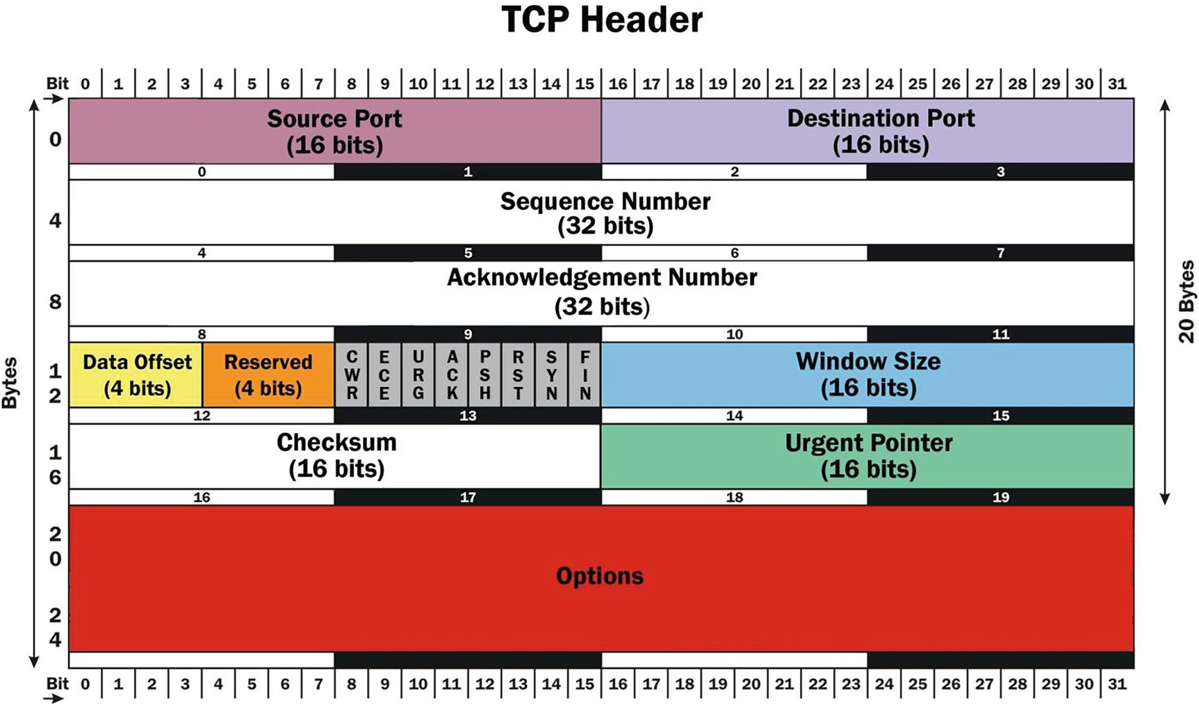
An illustration of the T C P packet header containing six layers. The source and destination port details are present in the first layer.
TCP packet header
Source Port (16 bits): Specifies the port that the data was written to on the sending node.
Destination Port (16 bits): Specifies the port that the data will be read from on the receiving node.
If the SYN flag is set, this field contains the initial sequence number. The sequence number of the actual first data byte (and the acknowledgment number in the resulting ACK) will then be that value plus 1.
If the SYN flag is clear, this field contains the accumulated sequence number of the first data byte of this packet for the current session.
If the ACK flag is set, this field is the next sequence number that the receiver is expecting. This acknowledges receipt of all previous bytes.
If the ACK flag is clear, this field is not used.
Data Offset (4 bits): Specifies the size of the TCP header in 32-bit words. The minimum value is 5 words (20 bytes), and the maximum value is 15 words (60 bytes), allowing for up to 40 bytes of options.
Reserved (4 bits): Not currently used and must be zeros.
CWR: Congestion Window Reduced. If set by the sender, it indicates it has received a TCP segment with the ECE flag set and has responded in a congestion control mechanism.
ECE: ECN Echo. If the SYN flag is set, then ECE set indicates that the TCP peer is ECN capable. If the SYN flag is clear, then the ECE flag set indicates that a Congestion Experienced flag in the IP header set was received during normal transmission.
URG: Indicates whether the Urgent Pointer field is significant.
ACK: If set, indicates that the Acknowledgement Number field is significant. All packets after the initial SYN packet sent by a node should have this flag set.
PSH: Push flag. If set, asks to push any buffered data to the receiving application.
RST: Reset flag. If set, resets the connection.
SYN: Synchronize flag. If set, synchronizes sequence numbers. Only the first packet sent from each end should have this flag set.
FIN: Finished flag – if set, no more data is coming.
Window Size (16 bits): Size of the receive window, which is the number of bytes that the receiver is willing to receive.
Checksum (16 bits): Used for error checking of the TCP header and data.
Urgent Pointer (16 bits): If the URG flag is set, this is the offset from the sequence number indicating the last urgent data byte.
Options (from zero to ten 32-bit words): Optional, not commonly used – see RFC for details.
- 1.
Connection is established using a three-way handshake, which creates a virtual circuit.
- 2.
Data is transferred over the virtual circuit until connection is terminated.
- 3.
Connection termination closes the established virtual circuit and releases allocated resources.
- 1.
LISTEN: Wait for a connection request from a remote client.
- 2.
SYN-SENT: Wait for the remote peer to send back a segment with SYN and ACK flags set.
- 3.
SYN-RECEIVED: Wait for the remote peer to send back acknowledgment after sending back a connection.
- 4.
ESTABLISHED: The port is ready to exchange data with the remote peer.
- 5.
FIN-WAIT-1
- 6.
FIN-WAIT-2
- 7.
CLOSE-WAIT
- 8.
CLOSING
- 9.
LAST-ACK
- 10.
TIME-WAIT: Ensure the remote peer has received acknowledgment of the termination request (< 4 minutes).
- 11.
CLOSED

A flow chart depicts the T C P state transition diagram. It has numerous blocks connected by arrows.
TCP state transition diagram (from Wikipedia)
Notes
TCP uses sequence numbers to detect lost packets and/or reorder packets that arrive out of order. The cumulative acknowledgment scheme informs the sender that all packets up to the acknowledged sequence number have been received. Selective acknowledgment (RFC 2018 117) allows for optimization of this feature. Lost data is automatically retransmitted by the sender. End-to-end flow control provides for a mismatch in performance between sender and receiver. A sliding window algorithm allows multiple packets to be in progress, which increases efficiency. Recently, congestion control has been added into TCP to avoid network congestion.
TCP is very complicated. The good news is that when used over IPv6, TCP works essentially the same way. The very minor changes will be covered later.
UDP: The User Datagram Protocol
The User Datagram Protocol is defined in RFC 768,118 “User Datagram Protocol,” August 1980. Like TCP, it is also a Transport Layer 119 protocol. Unlike TCP, UDP implements an unreliable, connectionless model . When we say unreliable, we just mean that error detection and recovery are not built into the protocol, so it is up to the application to do any desired error detection and recovery. By connectionless, we mean that each transmission consists of a single (but complete) packet. In IPv4, a packet is typically 1508 bytes, but can be more or less. If you send a big packet, it will likely be fragmented somewhere along the way and reassembled at the other end. Each datagram is an atomic event, not connected to any other datagram. UDP does not handle streams of data (as is done with the connection-oriented model ). Software that uses UDP does not need to open or close a connection; it can simply read or write datagrams at any time, and each operation sends or receives one packet. This is a much simpler model than TCP, with less overhead. However, when using UDP you are responsible for doing certain things that TCP does for you, such as error detection and retransmission. UDP is often used for things like streaming audio or video. It is also used for DNS queries and responses and for TFTP 120 (Trivial File Transfer Protocol ).
Standards Relevant to UDP
RFC 768 , “User Datagram Protocol,” August 1980 (Standards Track)
RFC 2508 , “Compressing IP/UDP/RTP Headers for Low-Speed Serial Links,” February 1999 (Standards Track)
RFC 3095, “Robust Header Compression (ROHC): Framework and Four Profiles: RTP, UDP, ESP and Uncompressed,” July 2001 (Standards Track)
RFC 3828, “The Lightweight User Datagram Protocols (UDP-Lite),” July 2004 (Standards Track)
RFC 4019, “Robust Header Compression (ROHC): Profiles for User Datagram Protocol (UDP) Lite,” April 2005 (Standards Track)
RFC 4113 , “Management Information Base for User Datagram Protocol (UDP),” June 2005 (Standards Track)
RFC 4362, “RObust Header Compression (ROHC): A Link-Layer Assisted Profile for IP/UDP/RTP,” January 2006 (Standards Track)
RFC 4727, “Experimental Values in IPv4, IPv6, ICMPv4, ICMPv6, UDP and TCP Headers,” November 2006 (Standards Track)
RFC 4815, “Robust Header Compression (ROHC): Corrections and Clarifications to RFC 3095,” February 2007 (Standards Track)
RFC 5097, “MIB for the UDP-Lite Protocol,” January 2008 (Standards Track)
RFC 5225, “RObust Header Compression Version 2 (ROHCv2): Profiles for RTP, UDP, IP, ESP and UDP-Lite,” April 2008 (Standards Track)
UDP Packet Header

A U D P header packet has three layers. The first layer has the source and destination port details. The next layer has length and checksum, and the final layer contains the data.
UDP packet header
The Source Port field (16 bits) specifies which port number the data is being written to on the sending computer. This field is optional (if not used, fill with zeros).
The Destination Port field (16 bits) specifies which port number the data is being read from on the receiving computer.
The Length field (16 bits) is the number of bytes in the datagram, including the UDP header and the data. Therefore, the minimum value is 8 (the length of the UDP header). The maximum value in theory is 65,536 bytes, but this value is limited by the maximum packet size, typically 1508.
- 1.
A “pseudo header,” which contains the source and destination IP addresses, the protocol number, and the UDP length (from the IP header)
- 2.
The UDP header itself
- 3.
The data, padded with a zero byte if required to make an even number of bytes
The Checksum field is optional (if not used, fill with zeros).
The Data field begins immediately after the Checksum field. It is not really part of the header, but it is factored into the checksum.
DHCPv4: Dynamic Host Configuration Protocol for IPv4
One of the network services that is really useful in network configuration is the Dynamic Host Configuration Protocol (DHCP 121) . The version that works with IPv4 is now called DHCPv4 (to distinguish it from the one for IPv6, which is called DHCPv6). DHCPv4 is specified in RFC 2131,122 “Dynamic Host Configuration Protocol,” March 1997. Without DHCPv4 running on your network, someone must manually configure all IPv4 network settings on every computer. This can be very complicated and error-prone. It also requires at least some expertise, which many users don’t possess. It is possible to accidently configure two computers with the same address or mistype a DNS server’s address on the 35th computer you install that day. These kinds of errors can cause tricky problems. With a DHCPv4 server, you can configure all the client computers to do “autoconfiguration.” When such a computer powers up, it will search for a DHCPv4 server (or a relay agent, connected to a real DHCPv4 server in another network). When it finds one, it will request configuration data (including the default gateway, the IP addresses of the DNS servers, the Internet domain name, and other items, including a lease on an IPv4 address, which should be unique within your network). This makes it easier to change things. If you move a DNS server or make other changes, you need only update your DHCPv4 server configuration and terminate all client leases (all nodes will request new configuration information).
DHCPv4 is widely used by ISPs, especially ones that have lots more customers than valid (globally routable) IPv4 addresses. They can set very short lease times. Then when someone disconnects, the address they had been using can be reused by another customer. Of course, these days, most people want 7×24 Internet connectivity, as opposed to perhaps 1 hour a day or dial-up access. Many ISPs now provide their customers with RFC 1918 private addresses, unless for some reason they specifically require a globally routable address. Some ISPs charge more for a globally routable address and a lot more for multiple globally routable addresses. I have one real public IPv4 address for my home network, so I can run email and other services, in addition to using one to tunnel IPv6 into my network over IPv4. DHCPv4 can provide autoconfiguration with private addresses just as easily as with globally routable addresses, so they still use DHCPv4 to assign those. Basically, all their users are now “hiding” behind a single public address, via NAT. More recently, users are behind two layers of NAT – they don’t even have one public IPv4 address anymore. This is done with CGNAT (Carrier-Grade NAT 123), with one mapping from a public address at the ISP to one private address from 100.64/10 at the ISP and another from that private address to multiple RFC 1918 private addresses in their network.
DHCPv4 uses broadcast (which doesn’t exist in IPv6) and can only deliver 32-bit addresses (for the assigned IP address or things like DNS IP addresses), so it had to be completely rewritten for IPv6. The differences will be covered in Chapter 6.
Most client operating systems in use today (especially on personal computers) include a DHCPv4 client, including all versions of Windows, FreeBSD, Linux, Solaris, Mac OSX, etc. Even smartphones with Wi-Fi include a DHCPv4 client. In practice, DHCPv6 may not be widely used, as IPv6 addresses and even discovery of IPv6 addresses for DNS are more likely to be done via Stateless Address Autoconfiguration (SLAAC) than via DHCPv6 (see RFC 6106,124 “IPv6 Router Advertisement Options for DNS Configuration”, November 2010).
Most server operating systems (such as Windows Server, FreeBSD, Linux, etc.) include a DHCPv4 server. The most common one for UNIX and UNIX-like servers is dhcpd from the Internet Systems Corporation (ISC) . It is configured by editing some complex ASCII text configuration files (with a text editor). This type of configuration has not changed appreciably in 50 years (and you thought IPv4 was old). The DHCPv4 server included with Windows Server at least has a GUI configuration tool, which is much easier to use. Most appliances that provide DHCPv4 service include a GUI web-based configuration tool (as a “front end” to dhcpd, in most cases).
When you configure a DHCPv4 server, you typically configure one or more pools of addresses to be managed by that server. You can have more than one DHCPv4 server in a given network subnet, but the managed address ranges must not overlap. DHCPv4 clients cannot contact DHCPv4 servers on another subnet (on the other side of a router) directly (since DHCPv4 servers are found via broadcast). So you either need to have a DHCPv4 server (or at least a DHCPv4 relay agent) in every subnet (“broadcast domain”). You can create a “scope” on the server and configure the “stateless” items that it will use to autoconfigure clients, including the domain name, the subnet mask, the address of the default gateway, the IP addresses of two DNS servers, etc. There are dozens of things you can autoconfigure with DHCPv4. You also specify a range of addresses (e.g., 192.168.5.100 to 192.168.5.199) as a pool from which to lease addresses. You should not manually assign any of these addresses to other nodes. If you do for some reason, you can exclude that address from the available pool.
Once such a server is installed and configured, just set up your client computers to “Obtain an IP address automatically” and to “Obtain DNS server address automatically.” As soon as you specify that or anytime the computer powers up, it will obtain all necessary information (including a unique IPv4 node address) from the DHCPv4 server. In Windows, you can use the “ipconfig /all” command (in a DOS prompt window) to view the obtained settings (look for the interface named Local Area Connection).
By default, addresses are assigned on a “first come, first served” basis. If you want a given node to be assigned a specific address each time, you can make an address reservation by associating one of the pool addresses with that node’s MAC address. Any time that node requests configuration data from the DHCPv4 server, it will be assigned the reserved address for that MAC address, rather than a random one from the pool.
The DHCPv4
- 1.
IP Discovery
- 2.
IP Lease Offer
- 3.
IP Request
- 4.
IP Lease Acknowledgment
Let’s say our network uses 192.168.0.0/16. That means the subnet mask is 255.255.0.0. Our DNS servers are at 192.168.0.11 and 192.168.0.12. The DHCPv4 server is also running on 192.168.0.11. The default gateway is 192.168.0.1. We have created a pool of addresses from 192.168.1.0 to 192.168.1.255.
Source address = 0.0.0.0, source port = 68
Destination address = 255.255.255.255, destination port = 67
DHCP option 50: IP address 192.168.1.100 is requested.
DHCP option 53: Message is DHCPDISCOVER.
Request subnet mask, default gateway, domain name, and domain name server(s).
In this case, the node is requesting its last known IP address. Assuming it is still connected to the same network and the address is not already leased to someone else, the server may grant the request. Otherwise, the client will have to negotiate for a new address.
Source address = 192.168.0.11, source port = 67
Destination address = 255.255.255.255, destination port = 68
DHCP option 01: Subnet mask is 255.255.0.0.
DHCP option 03: Default gateway is 192.168.0.1.
DHCP option 06: IP addresses of DNS servers are 192.168.0.11 and 192.168.0.12.
DHCP option 51: Lease duration is 86400 seconds (1 day).
DHCP option 53: Message is DHCPOFFER.
DHCP option 54: IP address of the DHCP server is 192.168.0.11.
Source address = 0.0.0.0, source port = 68
Destination address = 255.255.255.255, destination port = 67
DHCP option 50: IP address 192.168.1.100 is requested.
DHCP option 53: Message is DHCPREQUEST.
DHCP option 54: IP address of the DHCP server is 192.168.0.11.
Source address = 192.168.0.11, source port = 67
Destination address = 255.255.255.255, destination port = 68
DHCP option 01: Subnet mask is 255.255.0.0.
DHCP option 03: Default gateway is 192.168.0.1.
DHCP option 06: IP addresses of DNS servers are 192.168.0.11 and 192.168.0.12.
DHCP option 51: Lease duration is 86400 seconds (1 day).
DHCP option 53: Message is DHCPACK.
DHCP option 54: IP address of the DHCP server is 192.168.0.11.
At this point, the client actually configures those values for its network interface and can begin using the network.
Useful Commands Related to DHCPv4
ipconfig /release: Release the assigned IPv4 address and de-configure network.
ipconfig /renew: Do a new configuration request for IPv4.
ipconfig /all: View all network configuration settings.

A windows screen presents the output of an all ipconfig command. It has 11 lines.
Output of the ipconfig /all command
IPv4 Network Configuration
Furthermore, assume the DHCPv4 server is correctly configured with this information and is managing the address range 192.168.1.0–192.168.1.255 (and that some leases have already been granted).
IPv4 node address
Subnet mask (or, equivalently, CIDR subnet mask length)
IPv4 address of the default gateway
IPv4 addresses of DNS servers
Nodename
DNS domain name
Manual Network Configuration
It is possible to perform IPv4 network configuration on a node manually, either by editing ASCII configuration files, as in FreeBSD or Linux, or via GUI configuration tools, as in Windows. If you have understood the material in this chapter, it should be fairly easy for you to configure your node(s). In most cases, if you have ISP service, the ISP will give you all the information necessary to configure your node(s).
Let’s configure a FreeBSD 7.2 node manually. Assign it the nodename “us1.redwar.org” and the IP address 192.168.0.13. The interface we are configuring has the FreeBSD name “vr0”.
You need to edit the following files (you will need root privilege to do this):
Auto Network Configuration Using DHCPv4
It is also possible for a node to be automatically configured if a DHCPv4 server (or relay agent) is available somewhere on the LAN (or possibly from the ISP). If you are deploying several nodes on a home network, it is likely that there is a DHCPv4 server in your home gateway/DSL modem.
Let’s configure a FreeBSD 7.2 node automatically using DHCPv4. Assign it the nodename “us1.redwar.org” and any IP address from DHCPv4. The interface we are configuring has the FreeBSD name “vr0”.
You need to edit the following file (you will need root privilege to do this):

A screenshot of the T C P slash I P v 4 network configuration page. On the right side, there are instructions for configuration.
TCP/IP network configuration – main tab

A screenshot of the T C P slash I P v 4 properties dialog box. On the right are instructions for the I P v 4 network configuration.
IPv4 network configuration – TCP/IPv4 Properties dialog

A screenshot of the T C P slash I P v 4 properties dialog box. On the right are instructions for manually setting up the I P v 4 network configuration.
TCP/IP network configuration – IPv4 manual configuration dialog

A screenshot of the T C P slash I P v 6 network configuration main page. On the right side, there are instructions for configuration.
TCP/IP network configuration main tab – select IPv6

A screenshot of the T C P slash I P v 6 properties dialog box. On the right are instructions for automatically setting up the I P v 6 network configuration.
TCP/IP network configuration – TCP/IPv6 automatic configuration

A screenshot of the T C P slash I P v 6 properties dialog box. On the right are instructions for manually setting up the I P v 6 network configuration.
TCP/IP network configuration – TCP/IPv6 manual configuration
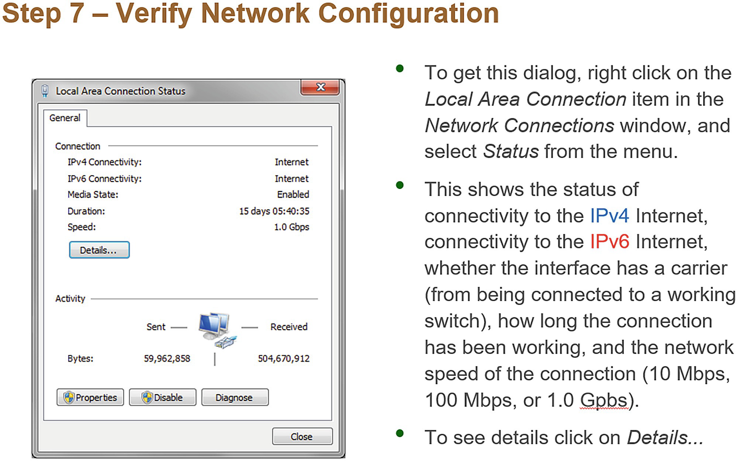
A screenshot of the local area connection status page. On the right, there are common instructions to verify I P v 4 and I P v 6 network configurations.
TCP/IP network configuration – verify configuration

A screenshot of the network connection details page. The common instructions to check the I P v 4 and I P v 6 network configurations are on the right.
TCP/IP network configuration – check network configuration details
Summary
In this chapter, we reviewed the technical aspects of IPv4. First off, some of you might not be familiar with the details of this protocol or how it has evolved over the many years since 1981, when it was specified.
In particular, we covered how we have “broken the Internet” by introducing NAT and private addresses and why it was done. This allowed us to keep using IPv4 well past its real shelf life, but at a very high cost (more complex network software design and limits on what most uses can do in terms of connections to and from other nodes). We have splintered the original IPv4 “monolithic address space” into millions of tiny “private Internets” loosely coupled together through NAT gateways.
There are many RFCs that specify how IPv4 works, going back to 1981 (RFCs 791 and 792).
Since IPv6 is heavily based on IPv4, you need to understand IPv4 in order to understand what is new in IPv6.
Likely, IPv4 will be phased out (at least at the international backbone level) in the next few years. Until then, we will have a global Internet that is partly IPv4 and partly IPv6. The two can exist in parallel, but it is not really practical to translate between them in either direction (NAT64 is very limited to allow translation from IPv6 addresses to external IPv4 servers).
If you are like most network engineers and developers today, you only know IPv4. If so, you are rapidly becoming obsolete. The future is IPv6. This book will help you make the leap from IPv4 to IPv6, so you will still have a job in a few years. Today, when I run into a corporate network that is IPv4-only, I feel like I am being asked to ride on a horse instead of my much more powerful and fast car (IPv6). The four-octet IPv4 addresses now look quaint and primitive to me, like the one-octet NDP addresses from ARPANET look to you now. Get used to 128-bit addresses in hexadecimal. The future is here.
A good analogy is when Novell NetWare was being replaced by TCP/IP some years ago. Many people were very tied to NetWare, with multiple certifications and extensive expertise, but soon there were no jobs for them. All networks were being converted over to TCP/IP because that was the native protocol of the Internet. They had to learn TCP/IP to be useful. The next generation has arrived.
If you want to have a good dose of reality, check out “Sunset IPv4” – the working group of the IETF whose charter was to figure out how to finally put IPv4 to sleep for good, like NetWare or OSI. So let us say a fond farewell to IPv4. The king is dead. Long live the king.