The Cyber Kill Chain

Developed by Lockheed Martin researchers to describe responses to advanced persistent threat (APT) attacks, the Cyber Kill Chain (CKC) methodology is based around the concept that attacks have multiple stages, and those stages can be associated with discrete, observable behaviors, leading to specific courses of actions for defense. The key idea of the CKC isn’t new (multistage models have been around for a long time), but it is critical for threat hunting—the attack takes multiple steps. In particular, there is a gap between the time that the attacker succeeds in infiltrating, and the time when the damage occurs.

While the original Intrusion Kill Chains are focused on APT, the same methodology can be applied to other classes of attacks. Figure 4-1 shows an example of the CKC multistage model and an application to APTs (the center column) and script kiddie attacks (right column). As the figure notes, in several stages, there is minimal expected difference between the two strategies—once an attacker is exploiting a host, the mechanism they used to get in is less of a barrier.

Kill Chains are a military concept; in the original paper, the authors create a very clever matrix relating courses of actions to the DoD’s IO actions: Detect, Deny, Disrupt, Degrade, Deceive, and Destroy. Linking observed phenomena, attacks, and courses of actions is an excellent product from a hunt, however the DoD IO framework is based around tools that the DoD has—in particular, the Destroy option¹ is out of the question. That said, deception is increasingly a viable approach with a number of companies playing in that field.²

Throughout the remainder of this chapter, I will refer to the terminology from the Cyber Kill Chain—the attack phases and the IO responses.

Figure 4-1. Examples of Kill Chains

Ranking Versus Detection

Lower tier analysis is usually expressed in terms of classification—intrusion detection, signatures, ways to definitively find a bad guy—which are then plugged into workflow. Hunters, being the people most likely to define these clean-cut cases, must first work with much more roughly defined data and vague phenomena. To that end, when hunters are developing tools for their own consumption, it’s preferable to think in terms of ranking rather than detection. By ranking, I mean ordering phenomena by likelihood and presenting that ordered list to spur further investigation.

For example, consider a situation where the hunter is looking to detect file exfiltration, and they’ve hit on two criteria: data volume and whether the targeted address is on a hitlist. The detection approach would involve creating a threshold, such as “more than 50 GB and target address on the hitlist,” then reporting any address above the threshold. The ranking approach would involve ordering the addresses, then returning that ordered list for further investigation.

The goal of ranking as opposed to simple detection is to identify cases that merit the analyst’s further attention. In a hunting process, you can do this by identifying cases that involve nonmalicious and repeatable anomalies, then pulling them away from the analyst’s direct attention. For example, in the file exfiltration case discussed, we may see backup servers copying traffic, we may see regular transfer to caches, we may see web proxies—all phenomena that on a well-behaved network should be somewhat manageable via a watchlist. When developing ranking systems, think about how the analyst will use the data after ranking, and whether there is additional data you can pull to help this. For example:

• If you’re returning an IP address, get further information. IP addresses are almost totally useless without context, so save the analyst a couple of steps by prefetching that context for them. If it’s internal, find out who owns it, and if it’s external, use geolocation or other labeling from threat intelligence.

• If you’re looking at something like volumes over time, provide some historical information—what happened yesterday, last week. If you’re looking at days of the week, note if it’s on the weekend or not.

• If you’re looking at some fraction of a larger set of traffic (for example, weird HTTP traffic among all HTTP traffic), include that context—how much of the total traffic does this amount make up?

The second element in this process is the metric itself, how you’re deciding to order the results. If you’re dealing with a single dimension (e.g., just volume or packet count), this is usually easy—bigger is near the top of the list, smaller near the bottom; pick your metric so bigger is weirder. When you’re dealing with multiple metrics, first normalize them (so that minimums and maximums have comparable values), then just add them together. For exploratory analysis, simple addition, or reasonable first step to get a console working, just recognize that it is an enormous kludge.

As an example of how all this behavior ties together, consider the example dashboard in Figure 4-2. This ties together several key points:

• Note that the dashboard has a central visualization, and that anomaly detection is applied to the dashboard. The red lines in the visualization indicate anomalies, while the horizontal line indicates the threshold for anomalous behavior.

• Anomalous behavior has been prefetched and pre-analyzed for the analysts. The list at the bottom corresponds to each anomaly and provides contextual information—how big the anomaly was, what hosts contributed to it, and when the anomaly occurred.

• Note that the dashboard has multiple top-n lists; there’s a master list on the right with all the hosts, and then each anomaly gets its own top-n list. This enables the analyst to quickly compare the addresses in the master list with the individual events.

• Whitelisting is removed from the main view, but whitelisted addresses are not ignored. Note that whitelisted information is included, just not as much and with a lower priority.

Figure 4-2. An example dashboard

Finite Cases

A hypothetical example: let’s say that you needed to build a system to identify the country of origin of an aircraft carrier. You could start building a general system, or you could start with some library research and find out that there are 21 active aircraft carriers, they’re owned by 9 countries, and the US owns 11 of these carriers. There are 9 cases to consider, and if you just say “US” you’re good over half the time.

Imagining all the potential cases is a very common source of analysis paralysis. However, when working with the type of data we’re usually looking at, answers are usually dominated by logistical and design concerns that reduce what we’re looking to down to a common set of cases—there’s a limited number of protocols, there’s a limited number of exploits, there’s a limited number of platforms. Furthermore, in many cases the potential set of cases is dominated by a small set. This is one of those problems where your analysts would be well served by doing some basic research. Ask: “how many solutions can there be for this?” and look up the relevant manufacturers.

Searching and Cross-Source Correlation

At the heart of any threat hunting loop is pulling data, examining it, and evaluating it. This usually involves cross-correlating the data from multiple sources. Nine times out of ten, correlation is a cut and dried process—you look across the records for the same IP addresses and the same times, and you’re done. The bulk of this section is concerned with the one time out of ten when correlation is weird, at which point the relationship becomes a lot less certain and a lot more dependent on the hunter’s judgment.

The correlation process consists of three parts; given the record of an event that occurred at a particular time, between two addresses, find other instances of that event in other log records. The motivation for doing this is due to the data you can collect from different vantage points, as shown in Figure 4-3. The scenario shown in Figure 4-3 is common: you have an HTTP session that you can observe via tcpdump and via HTTP logs. Correlation will be necessary for several reasons:

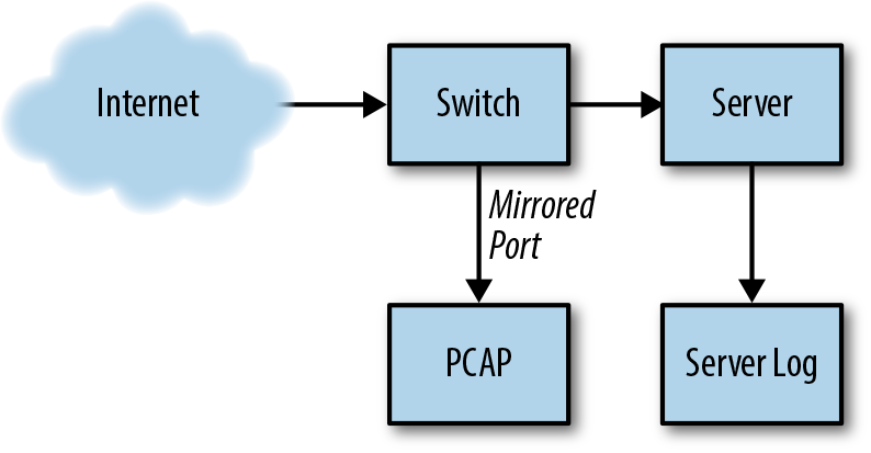
Figure 4-3. The vantage of network sensors and their impact on data collection

• You may not have access to the HTTP logs. The host may be an embedded device, or it may not be configured to record logs. Multiply this by hundreds or thousands of cases across your network.

• The service may be encrypted, such as HTTPS, in which case network collection is less directly valuable.

• The service may not be HTTP—the attacker may be using port 80 to evade your firewall, in which case the results will not appear in the server’s HTTP log.

Correlation starts with an event—you should have a time and a pair of addresses defining where the event came from and where it went to. For example, an HTTP request from 128.2.11.3 to 209.11.4.18 at 4:18 PM on Tuesday the 14th. Starting from this information, you look at all your other data sources in a similar time window and look for the same addresses. The factors that complicate this are how different systems record time, and how addresses may be changed en route.

Before assembling data for correlation, as part of your standard collection process, ensure that all the information you are using is synchronized and uses a common format. The first part of this (synchronization) is critical, so critical that I recommend creating heartbeat signals ahead of time (discussed in “Heartbeat Signals”) so that you can constantly verify and compensate for synchronization errors. The second part is critical for your sanity—if you have to constantly reformat timing data (and if you’re dealing with HTTP log files, you will), you will spend an inordinate amount of time double-checking results. On-the-fly reformatting wastes attention and introduces the risk of error; solve the problem before you hunt.

These steps are intended to ensure that whatever complications arise from data storage and formatting are addressed before you deal with the local and messy problems of how different systems model events, in particular, whether the event has a duration. If you’re looking at something like processor state, disk space, or individual packets, you’re looking at a sample that occurs instantly—start time and end time are the same. However, network sessions, flows, web pages, and the like, have a duration: they start at some time, and end at another time. Durations introduce a few distinct challenges:

• You need to know how a session ends. For most server logs, this is cut and dried, but NetFlow uses a timeout mechanism that can result in multiple flow records for a single session.

• Pay attention to how the logging system records these durations. If a session isn’t recorded until it terminates, you may never find log-based evidence for a long-lived session. Log systems that record session starts and ends are more useful for this purpose.

• You need to consider overlap. For example, if you record a page fetch from 10 to 14, and you have memory samples at 9, 11, 14, and 15, the samples at 11 and 14 may both be germane.

For these reasons, it’s better to work with time ranges rather than exact times. If you know that an event happened at time X, don’t just search for everything that happened at X, look between X–a, and X+a, where a is about as much additional time as you can computationally tolerate. The scope is going to drop as soon as you consider addressing anyway.⁴

For addressing, the cornerstone data is the 5-tuple: source IP address, destination IP address, source port, destination port, and protocol. When configuring log files, you should try to be able to infer a 5-tuple even if you can’t get the whole thing (for example, in the case of HTTP log files, you know the port from configuration and the protocol is always TCP, but you should add in the client port so you can reconstruct the whole 5-tuple). While the 5-tuple should be an exact match, there are elements which complicate it:

• NATting (network address translation) is generally the biggest confluence of common and obnoxious; if you have a NAT between one of your collection points then you have to be able to map the addresses. The NAT may have a log file that records this information, or it may dump a translation table at fixed intervals—in my experience, however, correlating across NATs is frustrating and manually intensive. This also applies for VPNs, load balancers, proxies, reverse proxies, MPLS, some too-clever-for-their-own-good firewalls, coloring, or any other technology that involves either manipulating addresses or rewriting packets.

• The 5-tuple is only meaningful for TCP and UDP, which have ports. You can still use source and destination IPs for most other protocols, although you should be cautious with ICMP—ICMP is an error-messaging protocol and an ICMP source address is often a piece of network hardware rather than the intended target.

• If you are working within the same VLAN, then MAC addresses are also a viable option. However, once a router enters the picture, then you are using IP addresses.

• If your timing information is imprecise, you can sometimes make up for timing by looking at ephemeral port assignments. IP stacks tend to assign port numbers linearly, so 2000, 2001, 2002, etc. If you need to figure out the order in which something happened and you don’t have enough precision in your timing, the ports might give you a way out.

Outside of the 5-tuple proper, you may want to use a number of different service-specific identifiers. These include, but aren’t limited to, domain names, active directory names, user IDs, email addresses, and MAC addresses. Many of these systems will behave in ways similar to IP addresses—they are hierarchical, there’s some kind of system for looking up relationships, and there are load-balancing systems that mess up the relationships. There are a a lot of ways to refer to an asset, and when managing a complex hunt, you may eventually find yourself juggling a number of different naming assets, at which point it is a good idea to create some lookup tables that link this information to randomly assigned UUIDs (universally unique identifiers). You can use the UUIDs as shorthand for the actual assets you’re looking for, and distinguish between the asset and all the observable information.

Lookup

Lookup is the process of figuring out where a network indicator (primarily IP addresses, although often names) is from—who owns it, for how long, and what for. Lookup is hard, and the results are rarely certain—as a rule of thumb, I assume that if I see an attack originating from some organization/country/company, that organization is likely uninvolved in the attack.

There are several common attribution searches, more than can be covered in this report: reverse lookups, WHOIS lookups, ASN lookups, and geolocation. None of these searches is perfect: the internet is designed on a store and forward model that relies on the destination address being legitimate, but doesn’t much care about the source address. This means that much of this data is not necessary for running the internet and is maintained by hand, where it’s subject to vigilance, honesty, and accurate recordkeeping.

Reverse lookups use DNS to trace the relationship between an IP address and a name. Reverse lookups are a part of the DNS protocol (e.g., you can run one using dig -x), but they are very much a kludge. There are multiple services (particularly CDNs and round robin allocation) that will break the reverse lookup relationship,⁵ as such, always do a forward lookup from the address the reverse lookup provides. The odds are that I am going to get a very different relationship, particularly if CDNs are involved.

A WHOIS lookup is a search for records in the WHOIS databases to provide information on who owns a particular domain. WHOIS information is intended to be human-readable, but the quality of it will vary based on vigilance and privacy constraints.⁶ While WHOIS can be done from the command line, it is a federated service and I find it’s generally more useful to go to one of the sources (e.g., http://whois.arin.net/ui/) directly and query from there.

An AS lookup will convert an IP address into an autonomous system number (ASN). ASes are address aggregates used for routing, and a basic structure for IP address allocation—that said, AS allocation is hierarchical in the sense that somebody might allocate an AS, then another one in that AS. There is no one tool for this process, but websites such as MxToolbox and Team Cymru are representative of lookup services that provide this information.

Finally, there’s geolocation. This is the relationship of an IP address to its physical location on the globe. There is no perfect geolocation, and frankly, outside of certain domains it isn’t very reliable at all, so before I say more be aware that this is very glitchy, uncertain, and you will have to be very careful.⁷ Geolocation is done by using databases manufactured by geolocation services such as Neustar, Dyn, and the like. These companies use a combination of internet-based research and physical investigation to determine address location, and in many cases provide additional information such as NAICS code, MSA,⁸ and the like. With geolocation services, you get what you pay for; I have used free data sources and found that I’ve spent more time manually vetting the results than I saved from the geolocation database. If you have the need for geolocation, and the resources, you buy a premium database. Period.

This leads to the final point of this brief section—I do not consider any source I have discussed in this section to be reliable. That doesn’t mean I won’t use them (I do, a lot), but it’s important to cross-correlate and compare information between these different sources all the time. You will get a result from a geolocation tool that tells you something is located in Germany, then do a WHOIS lookup to find it’s owned by a Canadian ISP, and then a reverse lookup that informs you that it’s a CDN. Trust nothing, buy quality sources, cross compare, and expect to use redundant versions of the same source.

Stack Counting

The most basic tool for identifying outliers in data is stack counting; stack counting is a technique applied to categorical data, and just consists of counting all the elements you see in each category, then ordering them to find the outliers (see Figure 4-4). At the command line, this is usually some incarnation of sort | uniq -c | sort -n, although your options vary by tool. Doing a count will give you a breakdown of tokens, order, and number.

In my experience, data in the output falls into four distinct categories: common phenomena, infrequent legitimate stuff, suspicious infrequent stuff, and errors. For the purposes of the remainder of this discussion, I will use HTTP User-Agent strings originating within an enterprise network. If you look at any enterprise site, you should expect that the overwhelming majority of the User-Agent strings are going to come from whatever browsers you run inside. You may well see over half of your traffic coming from one type of browser; you will almost certainly see less than a dozen different tokens making up the majority of your data.

Figure 4-4. Examples of stack counting

After this initial set, you should see a smaller set of tokens that appear regularly. Again, using the User-Agent example, these will include older browsers, as well as a number of things like embedded devices and apps that you don’t generally think of as a browser.

The third and fourth categories are where things get interesting. I’ll talk about the end first—often, the singletons are errors rather than actual malicious indicators. Examples of errors include partial packets, parsing errors, or just glitches in the collection system itself. The point is that if you see something once it may very well be false positive. The other category, more interesting, is when you see multiple sessions of things that you haven’t seen before, for example, User-Agent strings that almost look like legitimate User-Agent strings but only come from one host. Figure 4-5 discusses this more visually.

Stack counting is a good example of the use of ranking as opposed to detection; the categories in the preceding breakdown also suggest particular rules for examining the data to determine if there are additional suspicious actions. Other techniques to use include:

Checking to see if something is off about your common tokens

By definition, these values should be things that everybody uses, and if you see a string that appears there you’ve never heard of, you should find out what it is.

Movement between categories

You should expect the left end (frequently encountered elements) to be static—things just aren’t going to change that much. As you move rightward, there will be more churn—often times, it’s less the top 10 that’s interesting and more how fast things are climbing in the middle.

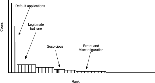
Figure 4-5. A rough breakdown of phenomena by frequency

Histograms and Barplots

You use stack counting when you’re working with unorderable categorical data. When you have some kind of ordering, you can move into histograms and barplots. Histograms and barplots are a similar looking plot for different data—histograms are used for ratio data (that is, continuous numerical values), and barplots for ordered categorical data. For the remainder of this section, I’m going to refer to everything as a histogram.

Figure 4-6 is an example showing the comparison of two histograms; in this case, the histograms represent the volume of traffic seen in short-lived HTTP and BitTorrent sessions. As this example shows, the difference between expected values is obvious, and a well-chosen histogram will often show these types of obvious results.

When looking at histograms, the first thing to do is identify peaks; these are a good place to focus analyst attention to determine why those peaks are occurring. For example, the significant peak at 88 bytes for BitTorrent in Figure 4-6 is a result of BitTorrent using a distinctively sized packet to determine whether the peer has a relevant file slice. Most of the time, the session returns negative and terminates immediately afterwards, resulting in this distinctive peak.

Figure 4-6. An example histogram comparing BitTorrent and HTTP expected session sizes

Apart from guiding attention, histograms are also a good tool for automated comparisons. As the example in Figure 4-6 shows, short-lived HTTP and BitTorrent sessions don’t look alike, and a user intending to masquerade BitTorrent as web surfing is going to have a hard time of it. Histogram comparison is a common research topic,⁹ and so there are a variety of different approaches depending on the data, precision requirements, and assumptions. For the purposes of this discussion, I am going to recommend the simplest approach, called L1 or Manhattan distance. For two normalized histograms, A and B, with bins from 0 to n, the Manhattan distance is:

Note the term “normalized” here; histograms are normally expressed as probability mass functions—the sum total of the heights is 1. Without accounting for the heights relative to each other, your results are likely to be useless.

Indicator Webwalk

Watchlists and indicator management will primarily work to reduce the number of hosts that an analyst is looking at, which raises the question of how do we add to that list of hosts? We do so primarily by looking at indicators of compromise (IOCs) and their spread throughout the network, a process that to me always resembles a spider walking across a web.

The indicator webwalk begins with a working set of suspicious hosts; these are hosts that the hunter believes are compromised to some degree.

1. The hunter pulls a host from the working set.

2. The hunter examines the host’s traffic and behavior to determine if it’s compromised.

   1. If the hunter believes the host is compromised, the hunter drops the host into a set of known bad hosts.

   2. If the hunter believes the host is not compromised, the hunter drops the host into a set of presumed good hosts.

   3. If the host is bad, the hunter identifies extracts new IOCs from the host and runs them across the remaining unknown hosts.

      1. Hosts that show the new IOCs are moved into the working set.

3. The process repeats until the working set is empty or the hunter runs out of time.

The heart of this process is a loop of examining a host for indicators of compromise, expanding the collection of indicators, and repeating the process. The most notable indicators in this process are communications patterns, for example:

• The compromised host speaks to a particular command and control server. Any other host that spoke to the C&C in the network is suspicious.

• The host drops a suspicious file on a fileshare. Any other host that copied that file is now suspicious.

Note also the use of the known bad and believed good categories. Hosts in this model are either guilty or not thoroughly examined.

Configuration Tracking and Baselining

There are two ways to determine whether behavior on a network is anomalous. In one approach, you collect observations about your network’s behavior and build statistical models to define normal and abnormal. In the second approach, you cheat. Cheating is good.

To cheat, engineer your network so that anomalous behavior is identifiable. In enterprise environments, this involves collecting inventories, generating baseline configurations, and tracking those baselines. Baseline configurations refer, basically, to whatever your IT department hands people when they get a new asset. For purposes of training and detection, consider the illustration in Figure 4-7—OEM, Baseline, User, and Power User.

• OEM systems are straight out of the factory and should have configurations straight out of the manual.

• Baseline systems refer to the configuration after your IT department gets a hold of the system. A hunter should be familiar with how the baseline differs from OEM—in particular, what additional software is added, what permissions are set up or removed, what security software is added, the network signatures of that software, and a list of all the potential software a user may add.

• User systems refer to the configuration after the user has gotten a hold of it. This should deviate from the baseline configuration, but it should be a manageable and largely additive deviation—the user adds new software such as productivity suites but does not, for example, spend a lot of time fiddling in the Windows directory. For the hunter, it’s better to think of the user space as a potential set of configurations rather than individual hosts. The hunter should be aware of things that a user may add that are not part of normally maintained software.

• Power Users is a bit glib here, but it refers to developers, system administrators, and any other user who has the knowledge and permission to develop or install arbitrary applications on their host. In the case of power users, the best the hunter can do is know that they exist, and that they will be the largest legitimate source of weirdness.

Figure 4-7. A reductive description of host complexity by user category

Honey

Once you have a trustworthy baseline, you can start to think about honeytokens. Honey is anything added to the system for the explicit purpose of detecting hostile probing or to frustrate attackers. The classic honey systems are honeypots, ersatz hosts that exist purely so that attackers contact them and waste time and reveal their techniques by controlling them. However, honey can be extended beyond that.

The basic criterion for honey is that it has to be something that is never used for legitimate purposes. It shouldn’t even be mentioned to the outside world, but instead left for attackers to find. Things that may be turned into honey include email addresses, credentials, websites, user accounts, and passwords. The key feature of honey is that legitimate users should never touch it (and outside of the administrators and security team, be unaware of it). That way, when the honey is tasted, admins know a priori it’s worth their attention.

Situational Awareness of Your Network: Mapping, Blindspots, Endpoint Detection

Inventory information is a constant output of the hunting process; your initial hunts will often turn into pure asset discovery as you find out that the traffic on your network is going to a huge number of resources you didn’t even know existed. As you do so, you should consider more systematic efforts to network mapping. This is a large topic, so I’m only going to touch on some basic principles here:

• Mapping can be done actively or passively. Passive mapping is done by examining the data you collect on the network as a matter of course, while active mapping is done by actively scanning and probing your network. The two techniques complement each other, as active mapping can be fine-tuned to specific problems, while passive mapping will point out things you didn’t know existed. A good starting point is to keep track of IP addresses and other information in your network passively, and when you see something you haven’t seen before, actively probe at it.

• Depending on the asset, you may be able to add local instrumentation, such as configuring its logs or adding an endpoint collection and analysis tool. Conversely, the asset may not have any instrumentation, in which case you may need to compensate by collecting right next to the asset.

• Pay particular attention to blindspots. Routing is self-healing, and that healing means that traffic may take strange, asymmetric paths through your network. If you see evidence of legitimate half-sessions (i.e., TCP sessions where you see only half of the client/server interaction, but it looks like it’s a real session), then there’s a good chance your network collection isn’t instrumenting every path.

• Pay attention to how the network looks from the outside world; external scanning, asset discovery services like Censys or Shodan, Alexa rankings, and Google Analysis are all tools. A good red team manual will provide you with a list of techniques.

• Guidance for future instrumentation is a common hunting output, and it’s often expensive and impractical to do everything at once. Keep a running list of what you’d like to collect or fix, and consider them as future projects.

Identifying Weird Port Behavior

Port assignments are an easily abused social convention; there is no central registry that requires that port 80 serve HTTP, there’s no requirement that port 80 be a server port. So, it’s chaos, it’s a fertile ground for attacker exploitation, and a good defender knows to check the ports for weirdness. These tips will help in finding the weird:

• Pay attention to whether the port is operating as a client or a server; in the case of TCP this is easily identified by looking at the flag combinations in the first packet. In the case of UDP, you’re going to have to look at spread—a server port will have a diverse set of IPs talking to it in a short period, while a client port is going to talk to one server and then pause for a while before being recycled. If a common server port is operating as a client, it’s a very good sign that someone’s trying to evade a firewall.

• Look for common packet and session sizes, especially with UDP-based services. Many services exchange packets with a very specific size or with some small degree of variation.¹⁰ When dealing with a new service, see if there are RFCs you can use to guess at the sizes.

• Often, the first 10–15 packets of a session are the most useful ones to look at. Many services are just a negotiation session leading up to a file transfer, so look at the negotiation for more information.

Producer/Consumer Ratio and Services

I broadly break services into a couple of categories: services that transfer control messages (NTP, BGP, SNMP), services that transfer files (SMTP, HTTP, FTP, some DNS), services that chat (IRC, XMPP, RabbitMQ), streamers (RTSP), and interactive services (SSH, telnet¹¹). These services tend to “look” different if you look at their packet sizes and interarrival times: control protocols have limited packet sizes and short exchanges, file transfer services tend to have a short negotiation, and then every packet is at MTU; chat services have short, different-sized packets, and a staccato back-and-forth; and interactive services go on for a long time with tiny packet sizes. Figuring out how to precisely express this is a work in progress, but one technique is the producer/consumer ratio (PCR).

The PCR is a metric developed by Carter Bullard and John Gerth for expressing the direction of network traffic. The PCR is defined as the ratio of difference of bytes from a source to a destination over the sum of bytes from a source to a destination (i.e., (SRC – DST)/(SRC + DST)); the intuition is that the lower the PCR, the more uploady the traffic is—a PCR of –1 indicates that traffic is a straight upload, while a PCR of 1 indicates the traffic is a straight download.

Know Your Calendar

Most enterprises will see their traffic follow the business cycle—that is, roughly from 9 to 5 daily on weekdays their traffic will peak, then lie fallow in the off hours. In addition, the characteristics of the traffic change. Activity during work hours is going to be human driven, while activity in the off hours is more likely to be automated.

In addition to this general shape, every organization has distinct holidays and business processing dates that are unique to the organization or its sector. Examples include:

National or local holidays

Holidays usually appear as “super weekends,” in the sense that they resemble weekend or off-hour traffic. The most useful detection tool for you in this group is the holiday unique to your organization—if you have special days dedicated to office retreats, founders days, or an out-of-country celebration, keep track of activity on that day.

Payment dates and payment processing

In general, anything that may require activity from internal accounting systems merits some study to determine how it works as a baseline. If you have internal accounting systems such as timecards, or an internal paystub server, note that the traffic there will tend to peak every two weeks.

Publishing reports or other outward-facing documents

If you are an organization that generally publishes reports (magazines, technology reports, annual studies), expect that activity will peak around those days.

Software releases, patch days

This particular calendar requires checking with your IT team, and in particular if their patching schedule is divorced from the main schedule. If the latter case is true, check theirs.

Knowing this traffic (start time, end time, volume of traffic, characteristic protocols) is a good start for understanding the normal traffic of your system. This is a rough-and-ready approach to time series analysis, and it does a disservice to compare it to more advanced techniques.

Of particular note when looking at timing is absence of evidence. If activity is regular, repeated, or predictable, then its absence should be a concern as much as too much activity. For example, a common attacker tactic is to disable antivirus; if you expect to see a regular AV update and hosts are missing from that update, it’s worth finding out why.

Watch Invocation Sequences

There are a lot of sequential operations in networks and on hosts that run predictably and regularly. This was generally observed by Forrest et al. in their seminal paper “A Sense of Self for Unix Processes.”¹² This general observation can be used in a number of different ways to find aberrant behavior; examples of this include:

• System applications: shells, daemons, servers. An exploit behavior is a shell launching from something that isn’t user interactive—if you see a shell launched from your PDF reader, isolate first and question later. Administrative processes are, in general, run predictably or auditably—the server launches on startup; if it launches in the middle of the day it’s because Administrator Bob had to mess with the system.

• Similarly, ssh and administrative traffic is often automated. On large networks, you’ll see administrative processes launch every hour, or every half an hour, predictably over the evenings.

• Web pages often require contacting multiple servers in an order specified by the information loaded. For example, an HTML page may load some JavaScript that, after the page is fully loaded, calls another server. This results in a specific sequence of pulls—the HTML page first, the server containing the JavaScript, and then the third server.

• DNS is another example of this kind of sequencing—almost all external traffic should require a DNS lookup. If you see contact with an IP address, and there’s no corresponding A record in your servers, that may mean caching, a manually modified hosts file, or someone entering an address by hand. All raise eyebrows.

There’s a couple of ways to leverage sequencing. For system administration application, it boils down to heuristics—track how shells are invoked, and if it’s off of a small list of allowed rules, make a note of it for further investigation. For sequences of servers, you can create a directed graph mapping out these dependencies, which can provide a visualization and comparison technique. In the case of network services, also be wary of caching, proxies, and other tools which may store the information, as they’ll mess with the sequence.

Be Aware of Physical Locations

A useful cue for anomalous activity is when it’s occurring from a location you wouldn’t expect. There are a number of tips for this kind of information that are worth keeping track of. These include:

Logins

If you see a user engaged in multiple redundant logins, it’s worth asking why.

Geolocation

Mobile monitoring packages will let you keep track of the physical coordinates of a device. Physical access logs such as card readers can help you get an idea of where a user is.

Language and preferences

Checking browser language preferences is an old trick for determining country of origin.

Physical locations are particularly important to consider when working with embedded and mobile devices.

Approximate String Matching

These are techniques that refer to matching strings that are close, but not exactly like each other. Approximate string matching techniques define a distance metric that explains how far away the strings are from each other—usually zero means an exact match, and the values increase from there.

For the threat hunter, approximate string matching techniques help obscure some of the ways that attackers will deceive end users. Often, the attacker looks to place something that is close enough for the user to believe or the casual reviewer to skip over.

Broadly speaking, the threat hunter needs to consider two classes of string matching techniques. The first are actual algorithms for string matching and analysis, the second are the various ways that the strings they are looking at may be structured to also evade detection.

In the former class are string matching algorithms. There are a lot of string matching algorithms, a brief set of which I’m going to discuss next. When I’m discussing these metrics, I’m going to use the term token to refer interchangeably to bits, characters, or even complete words if they’re taken from a dictionary.

Jaccard metric

The Jaccard metric is the ratio of characters that appear in both strings over the characters that appear in either string. So the metric is 1 if the strings have the same character sets, and 0 if the strings have nothing in common. The Jaccard metric is purely concerned with presence or absence, not ordering or count—so “cat,” “tac,” “tact,” and “act” will all have a metric of 1 vis-a-vis each other. That said, it’s very quick to calculate.

Hamming distance

Hamming distances are a character-by-character comparison, and consist of a sum of the distances between the individual characters. For example, the bit strings 010 and 000 have a Hamming distance of 1, and the strings 000 and 101 have a Hamming distance of 2. Hamming distance requires that the strings be of identical length; if they aren’t, you have to establish some convention for padding the strings.

Levenshtein distance

The Levenshtein distance between two strings is measured by breaking the differences between the string into a set of simple operations—insertion, deletion, and substitution.

Here’s the thing: there are lot of approximate string matching algorithms—they’re bread and butter for bioinformaticists, so diving into more of them is your responsibility, threat hunter. What’s really important for the threat hunting side of the equation is how you combine these matching algorithms with some know-how about how the data is structured.

For approximate string matching, much of the task involves identifying the large, redundant chunks of information in the dataset and removing it. Much of this information is a result of the data you’re looking at having some kind of tree structure. For example, in URLs, you will want to separate out the domain name, tokenize the TLD, and focus primarily on the elements in the middle.

LRU Cache Depth Analysis

Cache depth analysis is a technique for checking locality, which refers to the likelihood that requests are going to be closely related in time. The idea behind locality is that, much like in stack counting, activity is dominated by a limited number of tokens at any time. You would use stack depth analysis when you’re dealing with a sequence of indicators, and want an indication for how much that sequence changes.

An LRU cache operates as shown in Figure 4-8. As this figure shows, the cache pushes elements in order, with additional behaviors:

• Only one instance of a particular token is in the stack at any time. So if you send 50 copies of the same token in order, it’s treated as one.

• The cache is fixed size (this is important); when you introduce a a new value to a filled cache, the least recently used value is ejected.

• If you push a value into the cache and it’s already present, that value is moved to the top of the cache.

Figure 4-8. An LRU stack in action

The net result of these behaviors is that the top of the cache is dominated by the most recently seen values, most of which are commonly accessed. You can control this cache by observing the rate of replacement (how often values are ejected out of the cache) as a function of the depth of the cache.

Leaky Buckets

Leaky bucket algorithms come from network queueing, and they’re effectively a counter. A leaky bucket is a counter that polls a system at fixed intervals (for example, every second or every token, the intervals don’t have to be synchronous, as long as they’re well defined). If the phenomenon the bucket is looking for is present, then the counter is incremented. If not, then the bucket is decremented every few intervals—the net result is that if you have an event that is concentrated in time, you’ll see the bucket’s count spike up. However, if an event is occurring infrequently, the bucket will tend towards zero. Figure 4-9 illustrates this result.

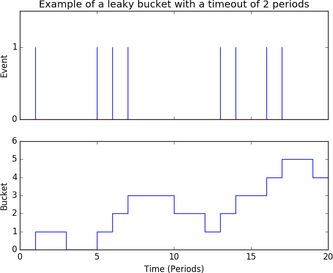
Figure 4-9. An example of a leaky bucket

Machine Learning

While specific machine learning techniques are outside the scope of this report, I can make several comments on machine learning and its relationship to threat hunting that will help inform the hunting process.

For threat hunters, machine learning is best treated as an undirected, exploratory analysis process. I have found that the most useful machine learning techniques in hunting are usually clustering techniques—a simple clustering approach such as k-means will help you organize data into discrete categories and guide further analysis. Be aware that applying machine learning to hunting is still manually intensive: the hours spent on machine learning primarily involve sanitizing and structuring data to feed into techniques.

A very common danger with machine learning techniques, and a reason for extreme conservatism, is that the more degrees of freedom you use in an algorithm, the more likely you are to concoct a story to justify a result.¹³ The problem is sufficiently well known that there are terms of art for it—p-hacking, in particular, refers to practices such as throwing variables into a regression analysis so that you’ll find a significant p-value through sheer chance.¹⁴

With all that said, some rules to keep in mind:

• I recommend learning k-means clustering, then regression, then ARIMA analysis. After that, go learn any techniques you like, but keep in mind that overly complex techniques lead to overfitting. As for why I recommend regression over ARIMA, it’s because everyone should know how linear regression works.

• Be conservative. Overfitting is a serious problem; if your solution is to fit hundreds of variables, rethink your premises. There’s a very real problem of p-hacking with excessive variables.

• Machine learning is not a substitute for good data. Time spent improving the quality of data collected is time well spent.

• You will never find quality labeled training data, so stop asking for it. You can occasionally gin up some training sets in the lab (and you shouldn’t be afraid to use a lab to generate a representative set of samples), but attackers aren’t interested in creating distinctive sets for you to work with.

• Be aware that many data sets will be too small. Techniques like deep learning require millions of observations. If you say something like “machine learning to detect attack X,” be aware that attack X may be infrequent enough and change rapidly enough that by the time you have a reasonable set of observations, the attack is obsolete.

• Pay attention to the visualizations. You should expect primarily to use machine learning techniques as a guide for further investigations in your hunt. Learn to read a dendrogram.

Trellising and Sparklines

This is a sparkline: . It is a small plot intended to be injected into another report in order to provide contextual information. Sparklines are, more than anything else, compact; the most extensive sparkline I’ve created had three visually distinct elements, but it was a very effective way of providing information at a glance.

Sparklines are particularly useful when trellised. Trellising is a plotting technique that ties multiple plots together on a common axis. A good example of a trellis is shown in Figure 4-10, which plots all the variables in a data set against each other to determine if there are any relationships between the variables.

Figure 4-10. An example of a trellised plot

Trellising and sparklines are valuable tools for dashboard design, as they provide a compact and clean representation of multiple variables simultaneously. I prefer using these plots rather than information such as color, both for human factors reasons (such as red-green colorblindness), and for cleanliness—you can express the same information without multiple colored points overlapping each other.

Remember that the strength of these plots is that they enable you to plot information cleanly; the plot in Figure 4-10, for example, shares axes so they don’t have to be drawn on each individual element. Use tricks like that to reduce complexity.

Radial Plots

A radial plot, also called a spider plot, is a plot that maps attributes on a circle. Radial plots are particularly useful for visualizing cyclical phenomena, such as the activity per days of the week shown in Figure 4-11.

Figure 4-11. A radial plot example

Heat Mapping and Space Filling Curves

A heat map (choropleth) is a visualization technique that paints different values in a map with different colors based on the numerical value. For threat hunting, heat maps are a good way to measure the frequency of data across different categories, where the categories may be organizational features, geographic, or even things like time of day. An example heat map is shown in the CAIDA IPv4 Census, which uses color to show the densities of individual address blocks.

A minor headache with mapping out internal IP addresses is the need to handle the end of the grid. For example, if you have a 16×16 grid, IP addresses 15 and 16 are going to end up in columns on either side of the map, even though they’re adjacent to each other. Another way to show this information is to use a space-filling curve, also called a Hilbert curve; this approach was popularized a few years by a map in Randall Munroe’s XKCD comic. The CAIDA IPv4 census I referred to is a mechanically generated version of that drawing. Hilbert curves will have uniformly sized cells, and they maintain adjacency, but it takes a while to build up the intuition for the various left and right turns, and the positioning changes the more information you add.

I slightly prefer space-filling curves over spirals, if only because the cells remain uniformly sized, however I feel that they’re generally best used at fixed cell counts and with extensive mapping. A guideline for the IP address and direction will make them much more usable.