© Akshay R Kulkarni, Adarsha Shivananda, Anoosh Kulkarni, V Adithya Krishnan 2023
A. R. Kulkarni et al.Time Series Algorithms Recipeshttps://doi.org/10.1007/978-1-4842-8978-5_1

1. Getting Started with Time Series

Akshay R Kulkarni1  , Adarsha Shivananda2, Anoosh Kulkarni3 and V Adithya Krishnan4
(1)
Bangalore, Karnataka, India
(2)
Hosanagara, Karnataka, India
(3)
Bangalore, India
(4)
Navi Mumbai, India
 

A time series is a sequence of time-dependent data points. For example, the demand (or sales) for a product in an e-commerce website can be measured temporally in a time series, where the demand (or sales) is ordered according to the time. This data can then be analyzed to find critical temporal insights and forecast future values, which helps businesses plan and increase revenue.

Time series data is used in every domain where real-time analytics is essential. Analyzing this data and forecasting its future value has become essential to these domains.

Time series analysis/forecasting was previously considered a purely statistical problem. It is now used in many machine learning and deep learning–based solutions, which perform equally well or even outperform most other solutions. This book uses various methods and approaches to analyze and forecast time series.

This chapter uses recipes to read/write time series data and perform simple preprocessing and Exploratory Data Analysis (EDA).

The following lists the recipes explored in this chapter.

  • Recipe 1-1. Reading Time Series Objects

  • Recipe 1-2. Saving Time Series Objects

  • Recipe 1-3. Exploring Types of Time Series Data

  • Recipe 1-4. Time Series Components

  • Recipe 1-5. Time Series Decomposition

  • Recipe 1-6. Visualization of Seasonality

Recipe 1-1A. Reading Time Series Objects (Air Passengers)

Problem

You want to read and load time series data into a dataframe.

Solution

Pandas load the data into a dataframe structure.

How It Works

The following steps read the data.

Step 1A-1. Import the required libraries.

import pandas as pd
import matplotlib.pyplot as plt

Step 1A-2. Write a parsing function for the datetime column.

Before reading the data, let’s write a parsing function.
date_parser_fn = lambda dates: pd.datetime.strptime(dates, '%Y-%m')

Step 1A-3. Read the data.

Read the air passenger data.
data = pd.read_csv('./data/AirPassenger.csv', parse_dates = ['Month'], index_col = 'Month', date_parser = date_parser_fn)
plt.plot(data)
plt.show()
Figure 1-1 shows the time series plot output.
Figure 1-1

Output

The following are some of the important input arguments for read_csv.
  • parse_dates mentions the datetime column in the dataset that needs to be parsed.

  • index_col mentions the column that is a unique identifier for the pandas dataframe. In most time series use cases, it’s the datetime column.

  • date_parser is a function to parse the dates (i.e., converts an input string to datetime format/type). pandas reads the data in YYYY-MM-DD HH:MM:SS format. Convert to this format when using the parser function.

Recipe 1-1B. Reading Time Series Objects (India GDP Data)

Problem

You want to save the loaded time series dataframe in a file.

Solution

Save the dataframe as a comma-separated (CSV) file.

How It Works

The following steps read the data.

Step 1B-1. Import the required libraries.

import pandas as pd
import matplotlib.pyplot as plt
import pickle

Step 1B-2. Read India’s GDP time series data.

indian_gdp_data = pd.read_csv('./data/GDPIndia.csv', header=0)
date_range = pd.date_range(start='1/1/1960', end='31/12/2017', freq='A')
indian_gdp_data ['TimeIndex'] = pd.DataFrame(date_range, columns=['Year'])
indian_gdp_data.head(5).T

Step 1B-3. Plot the time series.

plt.plot(indian_gdp_data.TimeIndex, indian_gdp_data.GDPpercapita)
plt.legend(loc='best')
plt.show()
Figure 1-2 shows the output time series.
Figure 1-2

Output

Step 1B-4. Store and retrieve as a pickle.

### Store as a pickle object
import pickle
with open('gdp_india.obj', 'wb') as fp:
        pickle.dump(IndiaGDP, fp)
### Retrieve the pickle object
with open('gdp_india.obj', 'rb') as fp:
     indian_gdp_data1 = pickle.load(fp)
indian_gdp_data1.head(5).T
Figure 1-3 shows the retrieved time series object transposed.
Figure 1-3

Output

Recipe 1-2. Saving Time Series Objects

Problem

You want to save a loaded time series dataframe into a file.

Solution

Save the dataframes as a CSV file.

How It Works

The following steps store the data.

Step 2-1. Save the previously loaded time series object.

### Saving the TS object as csv
data.to_csv('ts_data.csv', index = True, sep = ',')
### Check the obj stored
data1 = data.from_csv('ts_data.csv', header = 0)
### Check
print(data1.head(2).T)
The output is as follows.
1981-01-01
1981-01-02    17.9
1981-01-03    18.8
Name: 20.7, dtype: float64

Recipe 1-3A. Exploring Types of Time Series Data: Univariate

Problem

You want to load and explore univariate time series data.

Solution

A univariate time series is data with a single time-dependent variable.

Let’s look at a sample dataset of the monthly minimum temperatures in the Southern Hemisphere from 1981 to 1990. The temperature is the time-dependent target variable.

How It Works

The following steps read and plot the univariate data.

Step 3A-1. Import the required libraries.

import pandas as pd
import matplotlib.pyplot as plt

Step 3A-2. Read the time series data.

data = pd.read_csv('./data/daily-minimum-temperatures.csv', header = 0, index_col = 0, parse_dates = True, squeeze = True)
print(data.head())
The output is as follows.
Date
1981-01-01    20.7
1981-01-02    17.9
1981-01-03    18.8
1981-01-04    14.6
1981-01-05    15.8
Name: Temp, dtype: float64

Step 3A-3. Plot the time series.

Let’s now plot the time series data to detect patterns.
data.plot()
plt.ylabel('Minimum Temp')
plt.title('Min temp in Southern Hemisphere From 1981 to 1990')
plt.show()
Figure 1-4 shows the output time series plot.
Figure 1-4

Time series plot

This is called univariate time series analysis since only one variable, temp (the temperature over the past 19 years), was used.

Recipe 1-3B. Exploring Types of Time Series Data: Multivariate

Problem

You want to load and explore multivariate time series data.

Solution

A multivariate time series is a type of time series data with more features that the target depends on, which are also time-dependent; that is, the target is not only dependent on its past values. This relationship is used to forecast the target values.

Let’s load and explore a Beijing pollution dataset, which is multivariate.

How It Works

The following steps read and plot the multivariate data.

Step 3B-1. Import the required libraries.

import pandas as pd
from datetime import datetime
import matplotlib.pyplot as plt

Step 3B-2. Write the parsing function.

Before loading the raw dataset and parsing the datetime information as the pandas dataframe index, let’s first write a parsing function.
def parse(x):
    return datetime.strptime(x, '%Y %m %d %H')

Step 3B-3. Load the dataset.

data1 = pd.read_csv('./data/raw.csv',  parse_dates = [['year', 'month', 'day', 'hour']],
                   index_col=0, date_parser=parse)

Step 3B-4. Do basic preprocessing.

Drop the No column.
data1.drop('No', axis=1, inplace=True)
Manually specify each column name.
data1.columns = ['pollution', 'dew', 'temp', 'press', 'wnd_dir', 'wnd_spd', 'snow', 'rain']
data1.index.name = 'date'
Let’s mark all NA values with 0.
data1['pollution'].fillna(0, inplace=True)
Drop the first 24 hours.
data1 = data1[24:]
Summarize the first five rows.
print(data1.head(5))
The output is as follows.
                     pollution  dew  temp   press wnd_dir  wnd_spd  snow  rain
date
2010-01-02 00:00:00      129.0  -16  -4.0  1020.0      SE     1.79     0     0
2010-01-02 01:00:00      148.0  -15  -4.0  1020.0      SE     2.68     0     0
2010-01-02 02:00:00      159.0  -11  -5.0  1021.0      SE     3.57     0     0
2010-01-02 03:00:00      181.0   -7  -5.0  1022.0      SE     5.36     1     0
2010-01-02 04:00:00      138.0   -7  -5.0  1022.0      SE     6.25     2     0

This information is from a dataset on the pollution and weather conditions in Beijing. The time aggregation of the recordings was hourly and measured for five years. The data includes the datetime column, the pollution metric known as PM2.5 concentration, and some critical weather information, including temperature, pressure, and wind speed.

Step 3B-5. Plot each series.

Now let’s plot each series as a separate subplot, except wind speed direction, which is categorical.
vals = data1.values
# specify columns to plot
group_list = [0, 1, 2, 3, 5, 6, 7]
i = 1
# plot each column
plt.figure()
for group in group_list:
    plt.subplot(len(group_list), 1, i)
    plt.plot(vals[:, group])
    plt.title(data1.columns[group], y=0.5, loc='right')
    i += 1
plt.show()
Figure 1-5 shows the plot of all variables across time.
Figure 1-5

A plot of all variables across time

Recipe 1-4A. Time Series Components: Trends

Problem

You want to find the components of the time series, starting with trends.

Solution

A trend is the overall movement of data in a particular direction—that is, the values going upward (increasing) or downward (decreasing) over a period of time.

Let’s use a shampoo sales dataset, which has a monthly sales count for three years.

How It Works

The following steps read and plot the data.

Step 4A-1. Import the required libraries.

import pandas as pd
import matplotlib.pyplot as plt

Step 4A-2. Write the parsing function.

def parsing_fn(x):
    return datetime.strptime('190'+x, '%Y-%m')

Step 4A-3. Load the dataset.

data = pd.read_csv('./data/shampoo-sales.csv', header=0, parse_dates=[0], index_col=0, squeeze=True, date_parser= parsing_fn)

Step 4A-4. Plot the time series.

data.plot()
plt.show()
Figure 1-6 shows the time series plot.
Figure 1-6

Output

This data has a rising trend, as seen in Figure 1-6. The output time series plot shows that, on average, the values increase with time.

Recipe 1-4B. Time Series Components: Seasonality

Problem

You want to find the components of time series data based on seasonality.

Solution

Seasonality is the recurrence of a particular pattern or change in time series data.

Let’s use a Melbourne, Australia, minimum daily temperature dataset from 1981–1990. The focus is on seasonality.

How It Works

The following steps read and plot the data.

Step 4B-1. Import the required libraries.

import pandas as pd
import matplotlib.pyplot as plt

Step 4B-2. Read the data.

data = pd.read_csv('./data/daily-minimum-temperatures.csv', header = 0, index_col = 0, parse_dates = True, squeeze = True)

Step 4B-3. Plot the time series.

data.plot()
plt.ylabel('Minimum Temp')
plt.title('Min temp in Southern Hemisphere from 1981 to 1990')
plt.show()
Figure 1-7 shows the time series plot.
Figure 1-7

Output

Figure 1-7 shows that this data has a strong seasonality component (i.e., a repeating pattern in the data over time).

Step 4B-4. Plot a box plot by month.

Let’s visualize a box plot to check monthly variation in 1990.
month_df = DataFrame()
one_year_ser = data['1990']
grouped_df = one_year_ser.groupby(Grouper(freq='M'))
month_df = pd.concat([pd.DataFrame(x[1].values) for x in grouped_df], axis=1)
month_df = pd.DataFrame(month_df)
month_df.columns = range(1,13)
month_df.boxplot()
plt.show()
Figure 1-8 shows the box plot output by month.
Figure 1-8

Monthly level box plot output

The box plot, Figure 1-8, shows the distribution of minimum temperature for each month. There appears to be a seasonal component each year, showing a swing from summer to winter. This implies a monthly seasonality.

Step 4B-5. Plot a box plot by year.

Let’s group by year to see the change in distribution across various years. This way, you can check for seasonality at every time aggregation.
grouped_ser = data.groupby(Grouper(freq='A'))
year_df  = pd.DataFrame()
for name, group in grouped_ser:
    year_df[name.year] = group.values
year_df.boxplot()
plt.show()
Figure 1-9 shows the box plot output by year.
Figure 1-9

Yearly level box plot

Figure 1-9 reveals that there is not much yearly seasonality or trends in the box plot output.

Recipe 1-4C. Time Series Components: Seasonality (cont’d.)

Problem

You want to find time series components using another example of seasonality.

Solution

Let’s explore tractor sales data to understand seasonality.

How It Works

The following steps read and plot the data.

Step 4C-1. Import the required libraries.

import pandas as pd
import matplotlib.pyplot as plt

Step 4C-2. Read tractor sales data.

tractor_sales_data = pd.read_csv("./data/tractor_salesSales.csv")
tractor_sales_data.head(5)

Step 4C-3. Set a datetime series to use as an index.

date_ser = pd.date_range(start='2003-01-01', freq='MS', periods=len(Tractor))

Step 4C-4. Format the data.

tractor_sales_data.rename(columns={'Number of Tractor Sold':'Tractor-Sales'}, inplace=True)
tractor_sales_data.set_index(dates, inplace=True)
tractor_sales_data = tractor_sales_data[['Tractor-Sales']]
tractor_sales_data.head(5)

Step 4C-5. Plot the time series.

tractor_sales_data.plot()
plt.ylabel('Tractor Sales')
plt.title("Tractor Sales from 2003 to 2014")
plt.show()
Figure 1-10 shows the time series plot output.
Figure 1-10

Output

From the time series plot, Figure 1-10 shows that the data has a strong seasonality with an increasing trend.

Step 4C-6. Plot a box plot by month.

Let’s check the box plot by month to better understand the seasonality.
month_df = pd.DataFrame()
one_year_ser = tractor_sales_data['2011']
grouped_ser = one_year_ser.groupby(Grouper(freq='M'))
month_df = pd.concat([pd.DataFrame(x[1].values) for x in grouped_ser], axis=1)
month_df = pd.DataFrame(month_df)
month_df.columns = range(1,13)
month_df.boxplot()
plt.show()
Figure 1-11 shows the box plot output by month.
Figure 1-11

Monthly level box plot

The box plot shows a seasonal component each year, with a swing from May to August.

Recipe 1-5A. Time Series Decomposition: Additive Model

Problem

You want to learn how to decompose a time series using additive model decomposition.

Solution

  • The additive model suggests that the components add up.

  • It is linear, where changes over time are constantly made in the same amount.

  • The seasonality should have the same frequency and amplitude. Frequency is the width between cycles, and amplitude is the height of each cycle.

The statsmodel library has an implementation of the classical decomposition method, but the user has to specify whether the model is additive or multiplicative. The function is called seasonal_decompose.

How It Works

The following steps load and decompose the time series.

Step 5A-1. Load the required libraries.

### Load required libraries
import pandas as pd
import matplotlib.pyplot as plt
from statsmodels.tsa.seasonal import seasonal_decompose
import statsmodels.api as sm

Step 5A-2. Read and process retail turnover data.

turn_over_data = pd.read_csv('./data/RetailTurnover.csv')
date_range = pd.date_range(start='1/7/1982', end='31/3/1992', freq='Q')
turn_over_data['TimeIndex'] = pd.DataFrame(date_range, columns=['Quarter'])

Step 5A-3. Plot the time series.

plt.plot(turn_over_data.TimeIndex, turn_over_data.Turnover)
plt.legend(loc='best')
plt.show()
Figure 1-12 shows the time series plot output.
Figure 1-12

Time series plot output

Figure 1-12 shows that the trend is linearly increasing, and there is constant linear seasonality.

Step 5A-4. Decompose the time series.

Let’s decompose the time series by trends, seasonality, and residuals.
decomp_turn_over = sm.tsa.seasonal_decompose(turn_over_data.Turnover, model="additive", freq=4)
decomp_turn_over.plot()
plt.show()
Figure 1-13 shows the time series decomposition output.
Figure 1-13

Time series decomposition output

Step 5A-5. Separate the components.

You can get the trends, seasonality, and residuals as separate series with the following.
trend = decomp_turn_over.trend
seasonal = decomp_turn_over.seasonal
residual = decomp_turn_over.resid

Recipe 1-5B. Time Series Decomposition: Multiplicative Model

Problem

You want to learn how to decompose a time series using multiplicative model decomposition.

Solution

  • A multiplicative model suggests that the components are multiplied up.

  • It is non-linear, such as quadratic or exponential, which means that the changes increase or decrease with time.

  • The seasonality has an increasing or a decreasing frequency and/or amplitude.

How It Works

The following steps load and decompose the time series.

Step 5B-1. Load the required libraries.

### Load required libraries
import pandas as pd
import matplotlib.pyplot as plt
from statsmodels.tsa.seasonal import seasonal_decompose
import statsmodels.api as sm

Step 5B-2. Load air passenger data.

air_passengers_data = pd.read_csv('./data/AirPax.csv')

Step 5B-3. Process the data.

date_range = pd.date_range(start='1/1/1949', end='31/12/1960', freq='M')
air_passengers_data ['TimeIndex'] = pd.DataFrame(date_range, columns=['Month'])
print(air_passengers_data.head())
The output is as follows.
   Year Month  Pax  TimeIndex
0  1949   Jan  112 1949-01-31
1  1949   Feb  118 1949-02-28
2  1949   Mar  132 1949-03-31
3  1949   Apr  129 1949-04-30
4  1949   May  121 1949-05-31
Figure 1-14 shows the time series output plot.
Figure 1-14

Time series output plot

Step 5B-4. Decompose the time series.

decomp_air_passengers_data = sm.tsa.seasonal_decompose(air_passengers_data.Pax, model="multiplicative", freq=12)
decomp_air_passengers_data.plot()
plt.show()
Figure 1-15 shows the time series decomposition output.
Figure 1-15

Time series decomposition output

Step 5B-5. Get the seasonal component.

Seasonal_comp = decomp_air_passengers_data.seasonal
Seasonal_comp.head(4)
The output is as follows.
0    0.910230
1    0.883625
2    1.007366
3    0.975906
Name: Pax, dtype: float64

Recipe 1-6. Visualization of Seasonality

Problem

You want to learn how to visualize the seasonality component.

Solution

Let’s look at a few additional methods to visualize and detect seasonality. The retail turnover data shows the seasonality component per quarter.

How It Works

The following steps load and visualize the time series (i.e., the seasonality component).

Step 6-1. Import the required libraries.

import pandas as pd
import matplotlib.pyplot as plt

Step 6-2. Load the data.

turn_over_data = pd.read_csv('./data/RetailTurnover.csv')

Step 6-3. Process the data.

date_range = pd.date_range(start='1/7/1982', end='31/3/1992', freq='Q')
turn_over_data['TimeIndex'] = pd.DataFrame(date_range, columns=['Quarter'])

Step 6-4. Pivot the table.

Now let’s pivot the table such that quarterly information is in the columns, yearly information is in the rows, and the values consist of turnover information.
quarterly_turn_over_data = pd.pivot_table(turn_over_data, values = "Turnover", columns = "Quarter", index = "Year")
quarterly_turn_over_data
Figure 1-16 shows the output by quarterly turnover.
Figure 1-16

Quarterly turnover output

Step 6-5. Plot the line charts.

Let’s plot line plots for the four quarters.
quarterly_turn_over_data.plot()
plt.show()
Figure 1-17 shows the quarter-level line plots.
Figure 1-17

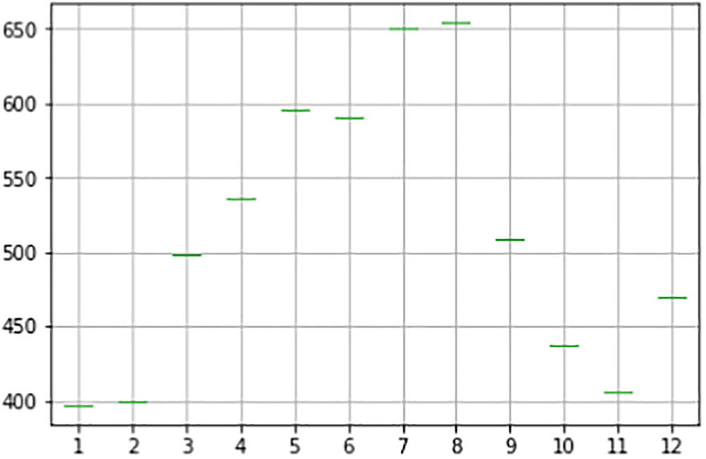
Quarterly turnover line chart

Step 6-6. Plot the box plots.

Let’s also plot the box plot at the quarterly level.
quarterly_turn_over_data.boxplot()
plt.show()
Figure 1-18 shows the output of the box plot by quarter.
Figure 1-18

Quarterly level box plot

Looking at both the box plot and the line plot, you can conclude that the yearly turnover is significantly high in the first quarter and is quite low in the second quarter.

..................Content has been hidden....................

You can't read the all page of ebook, please click here login for view all page.
Reset
3.140.188.16