© Akshay R Kulkarni, Adarsha Shivananda, Anoosh Kulkarni, V Adithya Krishnan 2023
A. R. Kulkarni et al.Time Series Algorithms Recipeshttps://doi.org/10.1007/978-1-4842-8978-5_2

2. Statistical Univariate Modeling

Akshay R Kulkarni1  , Adarsha Shivananda2, Anoosh Kulkarni3 and V Adithya Krishnan4
(1)
Bangalore, Karnataka, India
(2)
Hosanagara, Karnataka, India
(3)
Bangalore, India
(4)
Navi Mumbai, India
 

Univariate time series data analysis is the most popular type of temporal data, where a single numeric observation is recorded sequentially over equal time periods. Only the variable observed and its relation to time is considered in this analysis.

The forecasting of future values of this univariate data is done through univariate modeling. In this case, the predictions are dependent only on historical values. The forecasting can be done through various statistical methods. This chapter goes through a few important ones.

The following recipes for performing univariate statistical modeling are covered.
  • Recipe 2-1. Moving Average (MA) Forecast

  • Recipe 2-2. Autoregressive (AR) Model

  • Recipe 2-3. Autoregressive Moving Average (ARMA) Model

  • Recipe 2-4. Autoregressive Integrated Moving Average (ARIMA) Model

  • Recipe 2-5. Grid search Hyperparameter Tuning for Autoregressive Integrated Moving Average (ARIMA) Model

  • Recipe 2-6. Seasonal Autoregressive Integrated Moving Average (SARIMA) Model

  • Recipe 2-7. Simple Exponential Smoothing (SES) Model

  • Recipe 2-8. Holt-Winters (HW) Model

Recipe 2-1. Moving Average (MA) Forecast

Problem

You want to load time series data and forecast using a moving average.

Solution

A moving average is a method that captures the average change in a metric over time. For a particular window length, which is a short period/range in time, you calculate the mean target value, and then this window is moved across the entire period of the data, from start to end. It is usually used to smoothen the data and remove any random fluctuations.

Let’s use the pandas rolling mean function to get the moving average.

How It Works

The following steps read the data and forecast using the moving average.

Step 1-1. Import the required libraries.

from pandas import read_csv, Grouper, DataFrame, concat
import matplotlib.pyplot as plt
from datetime import datetime

Step 1-2. Read the data.

The US GDP data is a time series dataset that shows the annual gross domestic product (GDP) value (in US dollars) of the United States from 1929 to 1991.

The following reads the US GDP data.
us_gdp_data = pd.read_csv('./data/GDPUS.csv', header=0)

Step 1-3. Preprocess the data.

date_rng = pd.date_range(start='1/1/1929', end='31/12/1991', freq='A')
print(date_rng)
us_gdp_data['TimeIndex'] = pd.DataFrame(date_rng, columns=['Year'])
The output is as follows.
DatetimeIndex(['1929-12-31', '1930-12-31', '1931-12-31', '1932-12-31',
               '1933-12-31', '1934-12-31', '1935-12-31', '1936-12-31',
               '1937-12-31', '1938-12-31', '1939-12-31', '1940-12-31',
               '1941-12-31', '1942-12-31', '1943-12-31', '1944-12-31',
               '1945-12-31', '1946-12-31', '1947-12-31', '1948-12-31',
               '1949-12-31', '1950-12-31', '1951-12-31', '1952-12-31',
               '1953-12-31', '1954-12-31', '1955-12-31', '1956-12-31',
               '1957-12-31', '1958-12-31', '1959-12-31', '1960-12-31',
               '1961-12-31', '1962-12-31', '1963-12-31', '1964-12-31',
               '1965-12-31', '1966-12-31', '1967-12-31', '1968-12-31',
               '1969-12-31', '1970-12-31', '1971-12-31', '1972-12-31',
               '1973-12-31', '1974-12-31', '1975-12-31', '1976-12-31',
               '1977-12-31', '1978-12-31', '1979-12-31', '1980-12-31',
               '1981-12-31', '1982-12-31', '1983-12-31', '1984-12-31',
               '1985-12-31', '1986-12-31', '1987-12-31', '1988-12-31',
               '1989-12-31', '1990-12-31', '1991-12-31'],
              dtype='datetime64[ns]', freq='A-DEC')

Step 1-4. Plot the time series.

plt.plot(us_gdp_data.TimeIndex, us_gdp_data.GDP)
plt.legend(loc='best')
plt.show()
Figure 2-1 shows the time series plot output.
Figure 2-1

Output

Step 1-5. Use a rolling mean to get the moving average.

A window size of 5 is used for this example.
mvg_avg_us_gdp = us_gdp_data.copy()
#calculating the rolling mean - with window 5
mvg_avg_us_gdp['moving_avg_forecast'] = us_gdp_data['GDP'].rolling(5).mean()

Step 1-6. Plot the forecast vs. the actual.

plt.plot(us_gdp_data['GDP'], label='US GDP')
plt.plot(mvg_avg_us_gdp['moving_avg_forecast'], label='US GDP MA(5)')
plt.legend(loc='best')
plt.show()
Figure 2-2 shows the moving average (MA) forecast vs. the actual.
Figure 2-2

MA forecast vs. actual

Recipe 2-2. Autoregressive (AR) Model

Problem

You want to load the time series data and forecast using an autoregressive model.

Solution

Autoregressive models use lagged values (i.e., the historical values of a point to forecast future values). The forecast is a linear combination of these lagged values.

Let’s use the AutoReg function from statsmodels.tsa for modeling.

How It Works

The following steps load data and forecast using the AR model.

Step 2-1. Import the required libraries.

import pandas as pd
import numpy as np
import matplotlib.pyplot as plt
from statsmodels.tsa.stattools import adfuller
from statsmodels.tsa.ar_model import AutoReg
from statsmodels.graphics.tsaplots import plot_pacf

Step 2-2. Load and plot the dataset.

url='opsd_germany_daily.csv'
data = pd.read_csv(url,sep=",")
data['Consumption'].plot()
Figure 2-3 shows the plot of the time series data.
Figure 2-3

Output

Step 2-3. Check for stationarity of the time series data.

Let’s look for the p-value in the output of the Augmented Dickey-Fuller test. If the p-value is less than 0.05, the time series is stationary.
data_stationarity_test = adfuller(data['Consumption'], autolag='AIC')
print("P-value: ", data_stationarity_test[1])
The output is as follows.
P-value:  4.7440549018424435e-08

Step 2-4. Find the order of the AR model to be trained.

Let’s plot the partial autocorrelation function (pacf) plot to assess the direct effect of past data (lags) on future data.
pacf = plot_pacf(data['Consumption'], lags=25)
Figure 2-4 shows the output of the partial autocorrelation function plot.
Figure 2-4

Partial autocorrelation function plot

Figure 2-4 shows the partial autocorrelation function output and the number of lags until there is a significant partial correlation in the order of the AR model. In this case, it is 8.

Step 2-5. Create training and test data.

train_df = data['Consumption'][:len(data)-100]
test_df = data['Consumption'][len(data)-100:]

Step 2-6. Call and fit the AR model.

model_ar = AutoReg(train_df, lags=8).fit()

Step 2-7. Output the model summary.

print(ar_model.summary())
Figure 2-5 shows the AR model summary.
Figure 2-5

AR model summary

Step 2-8. Get the predictions from the model.

predictions = model_ar.predict(start=len(train_df), end=(len(data)-1), dynamic=False)

Step 2-9. Plot the predictions vs. actuals.

from matplotlib import pyplot
pyplot.plot(predictions)
pyplot.plot(test_df, color='red')
Figure 2-6 shows the predictions vs. actuals for the AR model.
Figure 2-6

Predictions vs. actuals

Recipe 2-3. Autoregressive Moving Average (ARMA) Model

Problem

You want to load time series data and forecast using an autoregressive moving average (ARMA) model.

Solution

An ARMA model uses the concepts of autoregression and moving averages to build a much more robust model. It has two hyperparameters (p and q) that tune the autoregressive and moving average components, respectively.

Let’s use the ARIMA function from statsmodels.tsa for modeling.

How It Works

The following steps load data and forecast using the ARMA model.

Step 3-1. Import the required libraries.

import pandas_datareader.data as web
import datetime
import pandas as pd
import numpy as np
from sklearn.metrics import mean_squared_error
import matplotlib.pyplot as plt
import seaborn as sns
from statsmodels.tsa.arima.model import ARIMA
from statsmodels.tsa.statespace.sarimax import SARIMAX
from statsmodels.tsa.api import SimpleExpSmoothing
from statsmodels.tsa.holtwinters import ExponentialSmoothing
import warnings

Step 3-2. Load the data.

Let’s use the bitcoin price (in USD) data from December 31, 2017, to January 4, 2018.
btc_data = pd.read_csv("btc.csv")
print(btc_data.head())
The output is as follows.
         Date       BTC-USD
0  2017-12-31  14156.400391
1  2018-01-01  13657.200195
2  2018-01-02  14982.099609
3  2018-01-03  15201.000000
4  2018-01-04  15599.200195

Step 3-3. Preprocess the data.

btc_data.index = pd.to_datetime(btc_data['Date'], format='%Y-%m-%d')
del btc_data['Date']

Step 3-4. Plot the time series.

plt.ylabel('Price-BTC')
plt.xlabel('Date')
plt.xticks(rotation=45)
plt.plot(btc_data.index, btc_data['BTC-USD'], )
Figure 2-7 shows the time series plot for the bitcoin price data.
Figure 2-7

Bitcoin price data

Step 3-5. Do a train-test split.

train_data = btc_data[btc_data.index < pd.to_datetime("2020-11-01", format='%Y-%m-%d')]
test_data = btc_data[btc_data.index > pd.to_datetime("2020-11-01", format='%Y-%m-%d')]
print(train_data.shape)
print(test_data.shape)
The output is as follows.
(1036, 1)
(31, 1)

Step 3-6. Plot time the series after the train-test split.

plt.plot(train_data, color = "black", label = 'Train')
plt.plot(test_data, color = "green", label = 'Test')
plt.ylabel('Price-BTC')
plt.xlabel('Date')
plt.xticks(rotation=35)
plt.title("Train/Test split")
plt.show()
Figure 2-8 shows the output time series plot after the train-test split.
Figure 2-8

Train-test split output

Step 3-7. Define the actuals from training.

actuals = train_data['BTC-USD']

Step 3-8. Initialize and fit the ARMA model.

ARMA_model = ARIMA(actuals, order = (1, 0, 1))
ARMA_model = ARMA_model.fit()

Step 3-9. Get the test predictions.

predictions = ARMA_model.get_forecast(len(test_data.index))
predictions_df = predictions.conf_int(alpha = 0.05)
predictions_df["Predictions"] = ARMA_model.predict(start = predictions_df.index[0], end = predictions_df.index[-1])
predictions_df.index = test_data.index
predictions_arma = predictions_df["Predictions"]

Step 3-10. Plot the train, test, and predictions as a line plot.

plt.plot(train_data, color = "black", label = 'Train')
plt.plot(test_data, color = "green", label = 'Test')
plt.ylabel('Price-BTC')
plt.xlabel('Date')
plt.xticks(rotation=35)
plt.title("ARMA model predictions")
plt.plot(predictions_arma, color="red", label = 'Predictions')
plt.legend()
plt.show()
Figure 2-9 shows the predictions vs. actuals for the ARMA model.
Figure 2-9

Predictions vs. actuals output

Step 3-11. Calculate the RMSE score for the model.

rmse_arma = np.sqrt(mean_squared_error(test_data["BTC-USD"].values, predictions_df["Predictions"]))
print("RMSE: ",rmse_arma)
The output is as follows.
RMSE:  4017.145069637629

The RMSE (root-mean-square error) is very high, as the dataset is not stationary. You need to make it stationary or use the autoregressive integrated moving average (ARIMA) model to get a better performance.

Recipe 2-4. Autoregressive Integrated Moving Average (ARIMA) Model

Problem

You want to load time series data and forecast using an autoregressive integrated moving average (ARIMA) model.

Solution

An ARIMA model improves upon the ARMA model because it also includes a third parameter, d, which is responsible for differencing the data to get in stationarity for better forecasts.

Let’s use the ARIMA function from statsmodels.tsa for modeling.

How It Works

The following steps load data and forecast using the ARIMA model.

Steps 3-1 to 3-7 from Recipe 2-3 are also used for this recipe.

Step 4-1. Make the data stationary by differencing.

# differencing
ts_diff = actuals - actuals.shift(periods=4)
ts_diff.dropna(inplace=True)

Step 4-2. Check the ADF (Augmented Dickey-Fuller) test for stationarity.

# checking for stationarity
from statsmodels.tsa.stattools import adfuller
result = adfuller(ts_diff)
pval = result[1]
print('ADF Statistic: %f' % result[0])
print('p-value: %f' % result[1])
The output is as follows.
ADF Statistic: -6.124168
p-value: 0.000000

Step 4-3. Get the Auto Correlation Function and Partial Auto Correlation Function values.

from statsmodels.tsa.stattools import adfuller
lag_acf = acf(ts_diff, nlags=20)
lag_pacf = pacf(ts_diff, nlags=20, method='ols')

Step 4-4. Plot the ACF and PACF to get p- and q-values.
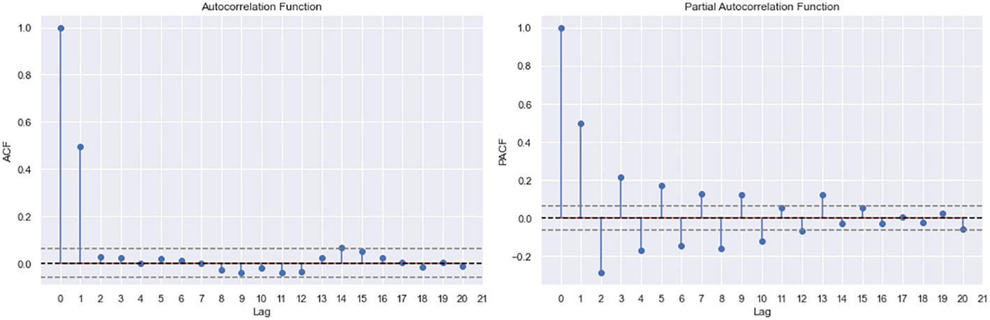
Plot the ACF and PACF to get the q- and p-values, respectively.
#Ploting ACF:
plt.figure(figsize = (15,5))
plt.subplot(121)
plt.stem(lag_acf)
plt.axhline(y = 0, linestyle='--',color='black')
plt.axhline(y = -1.96/np.sqrt(len(ts_diff)),linestyle='--',color='gray')
plt.axhline(y = 1.96/np.sqrt(len(ts_diff)),linestyle='--',color='gray')
plt.xticks(range(0,22,1))
plt.xlabel('Lag')
plt.ylabel('ACF')
plt.title('Autocorrelation Function')
#Plotting PACF:
plt.subplot(122)
plt.stem(lag_pacf)
plt.axhline(y = 0, linestyle = '--', color = 'black')
plt.axhline(y =-1.96/np.sqrt(len(actuals)), linestyle = '--', color = 'gray')
plt.axhline(y = 1.96/np.sqrt(len(actuals)),linestyle = '--', color = 'gray')
plt.xlabel('Lag')
plt.xticks(range(0,22,1))
plt.ylabel('PACF')
plt.title('Partial Autocorrelation Function')
plt.tight_layout()
plt.show()
Figure 2-10 shows the ACF and PACF plot outputs.
Figure 2-10

ACF and PACF plots

According to the ACF plot, the cutoff is 1, so the q-value is 1. According to the PACF plot, the cutoff is 10, so the p-value is 10.

Step 4-5. Initialize and fit the ARIMA model.

Using the derived p-, d-, and q-values.
ARIMA_model = ARIMA(actuals, order = (10, 4, 1))
ARIMA_model = ARIMA_model.fit()

Step 4-6. Get the test predictions.

predictions = ARIMA_model.get_forecast(len(test_data.index))
predictions_df = predictions.conf_int(alpha = 0.05)
predictions_df["Predictions"] = ARIMA_model.predict(start = predictions_df.index[0], end = predictions_df.index[-1])
predictions_df.index = test_data.index
predictions_arima = predictions_df["Predictions"]

Step 4-7. Plot the train, test, and predictions as a line plot.

plt.plot(train_data, color = "black", label = 'Train')
plt.plot(test_data, color = "green", label = 'Test')
plt.ylabel('Price-BTC')
plt.xlabel('Date')
plt.xticks(rotation=35)
plt.title("ARIMA model predictions")
plt.plot(predictions_arima, color="red", label = 'Predictions')
plt.legend()
plt.show()
Figure 2-11 shows the predictions vs. actuals for the ARIMA model.
Figure 2-11

Predictions vs. actuals output

Step 4-8. Calculate the RMSE score for the model.

rmse_arima = np.sqrt(mean_squared_error(test_data["BTC-USD"].values, predictions_df["Predictions"]))
print("RMSE: ",rmse_arima)
The output is as follows.
RMSE:  2895.312718157126

This model has performed better than an ARMA model due to the differencing part and finding the proper p-, d-, and q-values. But still, it has a high RMSE as the model is not perfectly tuned.

Recipe 2-5. Grid Search Hyperparameter Tuning for ARIMA Model

Problem

You want to forecast using an ARIMA model with the best hyperparameters.

Solution

Let’s use a grid search method to tune the model’s hyperparameters. The ARIMA model has three parameters (p, d, and q) that can be tuned using the classical grid search method. Loop through various combinations and evaluate each model to find the best configuration.

How It Works

The following steps load data and tune hyperparameters before forecasting using the ARIMA model.

Steps 3-1 to 3-7 from Recipe 2-3 are also used for this recipe.

Step 5-1. Write a function to evaluate the ARIMA model.

This function returns the RMSE score for a particular ARIMA order (input). It performs the same task as steps 3-8 and 3-9 in Recipe 2-3.
def arima_model_evaluate(train_actuals, test_data, order):
    # Model initalize and fit
    ARIMA_model = ARIMA(actuals, order = order)
    ARIMA_model = ARIMA_model.fit()
    # Getting the predictions
    predictions = ARIMA_model.get_forecast(len(test_data.index))
    predictions_df = predictions.conf_int(alpha = 0.05)
    predictions_df["Predictions"] = ARIMA_model.predict(start = predictions_df.index[0], end = predictions_df.index[-1])
    predictions_df.index = test_data.index
    predictions_arima = predictions_df["Predictions"]
    # calculate RMSE score
    rmse_score = np.sqrt(mean_squared_error(test_data["BTC-USD"].values, predictions_df["Predictions"]))
    return rmse_score

Step 5-2. Write a function to evaluate multiple models through grid search hyperparameter tuning.

This function uses the arima_model_evaluate function defined in step 5-8 to calculate the RMSE scores of multiple ARIMA models and returns the best model/configuration. It takes as input the list of p-, d-, and q-values that needs to be tested/experimented with.
def evaluate_models(train_actuals, test_data, list_p_values, list_d_values, list_q_values):
    best_rmse, best_config = float("inf"), None
    for p in list_p_values:
        for d in list_d_values:
            for q in list_q_values:
                arima_order = (p,d,q)
                rmse = arima_model_evaluate(train_actuals, test_data, arima_order)
                if rmse < best_rmse:
                    best_rmse, best_config = rmse, arima_order
                print('ARIMA%s RMSE=%.3f' % (arima_order,rmse))
    print('Best Configuration: ARIMA%s , RMSE=%.3f' % (best_config, best_rmse))
    return best_config

Step 5-3. Perform the grid search hyperparameter tuning by calling the defined functions.

p_values = range(0, 4)
d_values = range(0, 4)
q_values = range(0, 4)
warnings.filterwarnings("ignore")
best_config = evaluate_models(actuals, test_data, p_values, d_values, q_values)
The output is as follows.
ARIMA(0, 0, 0) RMSE=8973.268
ARIMA(0, 0, 1) RMSE=8927.094
ARIMA(0, 0, 2) RMSE=8895.924
ARIMA(0, 0, 3) RMSE=8861.499
ARIMA(0, 1, 0) RMSE=3527.133
ARIMA(0, 1, 1) RMSE=3537.297
ARIMA(0, 1, 2) RMSE=3519.475
ARIMA(0, 1, 3) RMSE=3514.476
ARIMA(0, 2, 0) RMSE=1112.565
ARIMA(0, 2, 1) RMSE=3455.709
ARIMA(0, 2, 2) RMSE=3315.249
ARIMA(0, 2, 3) RMSE=3337.231
ARIMA(0, 3, 0) RMSE=30160.941
ARIMA(0, 3, 1) RMSE=887.423
ARIMA(0, 3, 2) RMSE=3209.141
ARIMA(0, 3, 3) RMSE=2970.229
ARIMA(1, 0, 0) RMSE=4079.516
ARIMA(1, 0, 1) RMSE=4017.145
ARIMA(1, 0, 2) RMSE=4065.809
ARIMA(1, 0, 3) RMSE=4087.934
ARIMA(1, 1, 0) RMSE=3537.539
ARIMA(1, 1, 1) RMSE=3535.791
ARIMA(1, 1, 2) RMSE=3537.341
ARIMA(1, 1, 3) RMSE=3504.703
ARIMA(1, 2, 0) RMSE=725.218
ARIMA(1, 2, 1) RMSE=3318.935
ARIMA(1, 2, 2) RMSE=3507.106
ARIMA(1, 2, 3) RMSE=3314.726
ARIMA(1, 3, 0) RMSE=12360.360
ARIMA(1, 3, 1) RMSE=727.351
ARIMA(1, 3, 2) RMSE=2968.820
ARIMA(1, 3, 3) RMSE=3019.434
ARIMA(2, 0, 0) RMSE=4014.318
ARIMA(2, 0, 1) RMSE=4022.540
ARIMA(2, 0, 2) RMSE=4062.346
ARIMA(2, 0, 3) RMSE=4088.628
ARIMA(2, 1, 0) RMSE=3522.798
ARIMA(2, 1, 1) RMSE=3509.829
ARIMA(2, 1, 2) RMSE=3523.407
ARIMA(2, 1, 3) RMSE=3517.972
ARIMA(2, 2, 0) RMSE=748.267
ARIMA(2, 2, 1) RMSE=3498.685
ARIMA(2, 2, 2) RMSE=3514.870
ARIMA(2, 2, 3) RMSE=3310.798
ARIMA(2, 3, 0) RMSE=33486.993
ARIMA(2, 3, 1) RMSE=797.942
ARIMA(2, 3, 2) RMSE=2979.751
ARIMA(2, 3, 3) RMSE=2965.450
ARIMA(3, 0, 0) RMSE=4060.745
ARIMA(3, 0, 1) RMSE=4114.216
ARIMA(3, 0, 2) RMSE=4060.737
ARIMA(3, 0, 3) RMSE=3810.374
ARIMA(3, 1, 0) RMSE=3509.046
ARIMA(3, 1, 1) RMSE=3499.516
ARIMA(3, 1, 2) RMSE=3520.499
ARIMA(3, 1, 3) RMSE=3521.356
ARIMA(3, 2, 0) RMSE=1333.102
ARIMA(3, 2, 1) RMSE=3482.502
ARIMA(3, 2, 2) RMSE=3451.985
ARIMA(3, 2, 3) RMSE=3285.008
ARIMA(3, 3, 0) RMSE=14358.749
ARIMA(3, 3, 1) RMSE=1477.509
ARIMA(3, 3, 2) RMSE=3142.936
ARIMA(3, 3, 3) RMSE=2957.573
Best Configuration: ARIMA(1, 2, 0) , RMSE=725.218

Step 5-4. Initialize and fit the ARIMA model with the best configuration.

ARIMA_model = ARIMA(actuals, order = best_config)
ARIMA_model = ARIMA_model.fit()

Step 5-5. Get the test predictions.

predictions = ARIMA_model.get_forecast(len(test_data.index))
predictions_df = predictions.conf_int(alpha = 0.05)
predictions_df["Predictions"] = ARIMA_model.predict(start = predictions_df.index[0], end = predictions_df.index[-1])
predictions_df.index = test_data.index
predictions_arima = predictions_df["Predictions"]

Step 5-6. Plot the train, test, and predictions as a line plot.

plt.plot(train_data, color = "black", label = 'Train')
plt.plot(test_data, color = "green", label = 'Test')
plt.ylabel('Price-BTC')
plt.xlabel('Date')
plt.xticks(rotation=35)
plt.title("ARIMA model predictions")
plt.plot(predictions_arima, color="red", label = 'Predictions')
plt.legend()
plt.show()
Figure 2-12 shows the predictions vs. actuals for the ARIMA model.
Figure 2-12

Predictions vs. actuals output

Step 5-7. Calculate the RMSE score for the model.

rmse_arima = np.sqrt(mean_squared_error(test_data["BTC-USD"].values, predictions_df["Predictions"]))
print("RMSE: ",rmse_arima)
The output is as follows.
RMSE:  725.2180143501593

This is the best RMSE so far because the model is tuned and fits well.

Recipe 2-6. Seasonal Autoregressive Integrated Moving Average (SARIMA) Model

Problem

You want to load time series data and forecast using a seasonal autoregressive integrated moving average (SARIMA) model.

Solution

The SARIMA model is an extension of the ARIMA model. It can model the seasonal component of data as well. It uses seasonal p, d, and q components as hyperparameter inputs.

Let’s use the SARIMAX function from statsmodels.tsa for modeling.

How It Works

The following steps load data and forecast using the SARIMA model.

Steps 3-1 to 3-7 from Recipe 2-3 are also used for this recipe.

Step 6-1. Initialize and fit the SARIMA model.

SARIMA_model = SARIMAX(actuals, order = (1, 2, 0), seasonal_order=(2,2,2,12))
SARIMA_model = SARIMA_model.fit()

Step 6-2. Get the test predictions.

predictions = SARIMA_model.get_forecast(len(test_data.index))
predictions_df = predictions.conf_int(alpha = 0.05)
predictions_df["Predictions"] = SARIMA_model.predict(start = predictions_df.index[0], end = predictions_df.index[-1])
predictions_df.index = test_data.index
predictions_sarima = predictions_df["Predictions"]

Step 6-3. Plot the train, test, and predictions as a line plot.

plt.plot(train_data, color = "black", label = 'Train')
plt.plot(test_data, color = "green", label = 'Test')
plt.ylabel('Price-BTC')
plt.xlabel('Date')
plt.xticks(rotation=35)
plt.title("SARIMA model predictions")
plt.plot(predictions_sarima, color="red", label = 'Predictions')
plt.legend()
plt.show()
Figure 2-13 shows the predictions vs. actuals for the seasonal ARIMA model.
Figure 2-13

Predictions vs. actuals output

Step 6-4. Calculate the RMSE score for the model.

rmse_sarima = np.sqrt(mean_squared_error(test_data["BTC-USD"].values, predictions_df["Predictions"]))
print("RMSE: ",rmse_sarima)
The output is as follows.
RMSE:  1050.157033576061

You can further tune the seasonal component to get a better RMSE score. Tuning can be done using the same grid search method.

Recipe 2-7. Simple Exponential Smoothing (SES) Model

Problem

You want to load the time series data and forecast using a simple exponential smoothing (SES) model.

Solution

Simple exponential smoothing is a smoothening method (like moving average) that uses an exponential window function.

Let’s use the SimpleExpSmoothing function from statsmodels.tsa for modeling.

How It Works

The following steps load data and forecast using the SES model.

Steps 3-1 to 3-7 from Recipe 2-3 are also used for this recipe.

Step 7-1. Initialize and fit the SES model.

SES_model = SimpleExpSmoothing(actuals)
SES_model = SES_model.fit(smoothing_level=0.8,optimized=False)

Step 7-2. Get the test predictions.

predictions_ses = SES_model.forecast(len(test_data.index))

Step 7-3. Plot the train, test, and predictions as a line plot.

plt.plot(train_data, color = "black", label = 'Train')
plt.plot(test_data, color = "green", label = 'Test')
plt.ylabel('Price-BTC')
plt.xlabel('Date')
plt.xticks(rotation=35)
plt.title("SImple Exponential Smoothing (SES) model predictions")
plt.plot(predictions_ses, color='red', label = 'Predictions')
plt.legend()
plt.show()
Figure 2-14 shows the predictions vs. actuals for the SES model.
Figure 2-14

Predictions vs. actuals output

Step 7-4. Calculate the RMSE score for the model.

rmse_ses = np.sqrt(mean_squared_error(test_data["BTC-USD"].values, predictions_ses))
print("RMSE: ",rmse_ses)
The output is as follows.
RMSE:  3536.5763879303104

As expected, the RMSE is very high because it’s a simple smoothing function that performs best when there is no trend in the data.

Recipe 2-8. Holt-Winters (HW) Model

Problem

You want to load time series data and forecast using the Holt-Winters (HW) model.

Solution

Holt-Winters is also a smoothing function. It uses the exponential weighted moving average. It encodes previous historical values to predict present and future values.

For modeling, let’s use the ExponentialSmoothing function from statsmodels.tsa.holtwinters.

How It Works

The following steps load data and forecast using the HW model.

Steps 3-1 to 3-7 from Recipe 2-3 are also used for this recipe.

Step 8-1. Initialize and fit the HW model.

HW_model = ExponentialSmoothing(actuals, trend='add')
HW_model = HW_model.fit()

Step 8-2. Get the test predictions.

predictions_hw = HW_model.forecast(len(test_data.index))

Step 8-3. Plot the train, test, and predictions as a line plot.

plt.plot(train_data, color = "black", label = 'Train')
plt.plot(test_data, color = "green", label = 'Test')
plt.ylabel('Price-BTC')
plt.xlabel('Date')
plt.xticks(rotation=35)
plt.title("HW model predictions")
plt.plot(predictions_hw, color='red', label = 'Predictions')
plt.legend()
plt.show()
Figure 2-15 shows the predictions vs. actuals for the HW model.
Figure 2-15

Predictions vs. actuals output

Step 8-4. Calculate the RMSE score for the model.

rmse_hw = np.sqrt(mean_squared_error(test_data["BTC-USD"].values, predictions_hw))
print("RMSE: ",rmse_hw)
The output is as follows.
RMSE:  2024.6833967531811

The RMSE is a bit high, but for this dataset, the additive model performs better than the multiplicative model. For the multiplicative model, change the trend term to 'mul' in the ExponentialSmoothing function.

..................Content has been hidden....................

You can't read the all page of ebook, please click here login for view all page.
Reset
18.221.140.111