1 Understanding time series forecasting
- Introducing time series
- Understanding the three main components of a time series
- The steps necessary for a successful forecasting project
- How forecasting time series is different from other regression tasks
Time series exist in a variety of fields from meteorology to finance, econometrics, and marketing. By recording data and analyzing it, we can study time series to analyze industrial processes or track business metrics, such as sales or engagement. Also, with large amounts of data available, data scientists can apply their expertise to techniques for time series forecasting.
You might have come across other courses, books, or articles on time series that implement their solutions in R, a programming language specifically made for statistical computing. Many forecasting techniques make use of statistical models, as you will learn in chapter 3 and onwards. Thus, a lot of work was done to develop packages to make time series analysis and forecasting seamless using R. However, most data scientists are required to be proficient with Python, as it is the most widespread language in the field of machine learning. In recent years, the community and large companies have developed powerful libraries that leverage Python to perform statistical computing and machine learning tasks, develop websites, and much more. While Python is far from being a perfect programming language, its versatility is a strong benefit to its users, as we can develop models, perform statistical tests, and possibly serve our models through an API or develop a web interface, all while using the same programming language. This book will show you how to implement both statistical learning techniques and machine learning techniques for time series forecasting using only Python.
This book will focus entirely on time series forecasting. You will first learn how to make simple forecasts that will serve as benchmarks for more complex models. Then we will use two statistical learning techniques, the moving average model and the autoregressive model, to make forecasts. These will serve as the foundation for the more complex modeling techniques we will cover that will allow us to account for non-stationarity, seasonality effects, and the impact of exogenous variables. Afterwards, we’ll switch from statistical learning techniques to deep learning methods, in order to forecast very large time series with a high dimensionality, a scenario in which statistical learning often does not perform as well as its deep learning counterpart.
For now, this chapter will examine the basic concepts of time series forecasting. I’ll start by defining time series so that you can recognize one. Then, we will move on and discuss the purpose of time series forecasting. Finally, you will learn why forecasting a time series is different from other regression problems, and thus why the subject deserves its own book.
1.1 Introducing time series
The first step in understanding and performing time series forecasting is learning what a time series is. In short, a time series is simply a set of data points ordered in time. Furthermore, the data is often equally spaced in time, meaning that equal intervals separate each data point. In simpler terms, the data can be recorded at every hour or every minute, or it could be averaged over every month or year. Some typical examples of time series include the closing value of a particular stock, a household’s electricity consumption, or the temperature outside.
Let’s consider a dataset representing the quarterly earnings per share in US dollars of Johnson & Johnson stock from 1960 to 1980, shown in figure 1.1. We will use this dataset often throughout this book, as it has many interesting properties that will help you learn advanced techniques for more complex forecasting problems.
As you can see, figure 1.1 clearly represents a time series. The data is indexed by time, as marked on the horizontal axis. Also, the data is equally spaced in time, since it was recorded at the end of every quarter of each year. We can see that the data has a trend, since the values are increasing over time. We also see the earnings going up and down over the course of each year, and the pattern repeats every year.

Figure 1.1 Quarterly earnings of Johnson & Johnson in USD from 1960 to 1980 showing a positive trend and a cyclical behavior
1.1.1 Components of a time series
We can further our understanding of time series by looking at their three components: a trend, a seasonal component, and residuals. In fact, all time series can be decomposed into these three elements.
Visualizing the components of a time series is known as decomposition. Decomposition is defined as a statistical task that separates a time series into its different components. We can visualize each individual component, which will help us identify the trend and seasonal pattern in the data, which is not always straightforward just by looking at a dataset.
Let’s take a closer look at the decomposition of Johnson & Johnson quarterly earnings per share, shown in figure 1.2. You can see how the Observed data was split into Trend, Seasonal, and Residuals. Let’s study each piece of the graph in more detail.

First, the top graph, labeled as Observed, simply shows the time series as it was recorded (figure 1.3). The y-axis displays the value of the quarterly earnings per share for Johnson & Johnson in US dollars, while the x-axis represents time. It is basically a recreation of figure 1.1, and it shows the result of combining the Trend, Seasonal, and Residuals graphs from figure 1.2.

Then we have the trend component, as shown in figure 1.4. Again, keep in mind that the y-axis represents the value, while the x-axis still refers to time. The trend is defined as the slow-moving changes in a time series. We can see that it starts out flat and then steeply goes up, meaning that we have an increasing, or positive, trend in our data. The trend component is sometimes referred to as the level. We can think of the trend component as trying to draw a line through most of the data points to show the general direction of a time series.

Figure 1.4 Focusing on the trend component. We have a trend in our series, since the component is not flat. It indicates that we have increasing values over time.
Next we see the seasonal component in figure 1.5. The seasonal component captures the seasonal variation, which is a cycle that occurs over a fixed period of time. We can see that over the course of a year, or four quarters, the earnings per share start low, increase, and decrease again at the end of the year.

Figure 1.5 Focusing on the seasonal component. Here we have periodic fluctuations in our time series, which indicates that earnings go up and down every year.
Notice how the y-axis shows negative values. Does this mean that the earnings per share are negative? Clearly, that cannot be, since our dataset strictly has positive values. Therefore, we can say that the seasonal component shows how we deviate from the trend. Sometimes we have a positive deviation, and we get a peak in the Observed graph. Other times, we have a negative deviation, and we see a trough in Observed.
Finally, the last graph in figure 1.2 shows the residuals, which is what cannot be explained by either the trend or the seasonal components. We can think of the residuals as adding the Trend and Seasonal graphs together and comparing the value at each point in time to the Observed graph. For certain points, we might get the exact same value as in Observed, in which case the residual will be zero. In other cases, the value is different from the one in Observed, so the Residuals graph shows what value must be added to Trend and Seasonal in order to adjust the result and get the same value as in Observed. Residuals usually correspond to random errors, also termed white noise, as we will discuss in chapter 3. They represent information that we cannot model or predict, since it is completely random, as shown in figure 1.6.
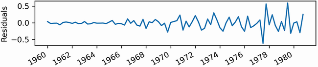
Figure 1.6 Focusing on the residuals. The residuals are what cannot be explained by the trend and seasonal components.
Already we can intuitively see how each component affects our work when forecasting. If a time series exposes a certain trend, then we’ll expect it to continue in the future. Similarly, if we observe a strong seasonality effect, this is likely going to continue, and our forecasts must reflect that. Later in the book, you’ll see how to account for these components and include them in your models to forecast more complex time series.
1.2 Bird’s-eye view of time series forecasting
Forecasting is predicting the future using historical data and knowledge of future events that might affect our forecasts. This definition is full of promises and, as data scientists, we are often very eager to start forecasting by using our scientific knowledge to showcase an incredible model with a near-perfect forecast accuracy. However, there are important steps that must be covered before reaching the point of forecasting.
Figure 1.7 is a simplified diagram of what a complete forecasting project might look like in a professional setting. Note that these steps are not universal, and they may or may not be followed, depending on the organization and its maturity. These steps are nonetheless essential to ensure good cohesion between the data team and the business team, hence providing business value and avoiding friction and frustration between the teams.

Figure 1.7 Forecasting project roadmap. The first step is naturally to set a goal that justifies the need for forecasting. Then you must determine what needs to be forecast in order to achieve that goal. Then you set the horizon of the forecast. Once that’s done, you can gather the data and develop a forecasting model. Then the model is deployed to production, its performance is monitored, and new data is collected in order to retrain the forecasting model and make sure it is still relevant.
Let’s dive into a scenario that covers each step of a forecasting project roadmap in detail. Imagine you are planning a one-week camping trip one month from now, and you want to know which sleeping bag to bring with you so you can sleep comfortably at night.
1.2.1 Setting a goal
The very first step in any project roadmap is to set a goal. Here it is explicit in the scenario: you want to know which sleeping bag to bring to sleep comfortably at night. If the nights will be cold, a warm sleeping bag is the best choice. Of course, if nights are expected to be warm, then a light sleeping bag would be the better option.
1.2.2 Determining what must be forecast to achieve your goal
Then you move to determining what must be forecast in order for you to decide which sleeping bag to bring. In this case, you need to predict the temperature at night. To simplify things, let’s consider that predicting the minimum temperature is sufficient to make a decision, and that the minimum temperature occurs at night.
1.2.3 Setting the horizon of the forecast
Now you can set the horizon of your forecast. In this case, your camping trip is one month from now, and it will last for one week. Therefore, you have a horizon of one week, since you are only interested in predicting the minimum temperature during the camping trip.
1.2.4 Gathering the data
You can now start gathering your data. For example, you could collect historical daily minimum temperature data. You could also gather data on possible factors that can influence temperature, such as humidity and wind speed.
This is when the question of how much data is enough data arises. Ideally, you would collect more than 1 year of data. That way, you could determine if there is a yearly seasonal pattern or a trend. In the case of temperature, you can of course expect some seasonal pattern over the year, since different seasons bring different minimum temperatures.
However, 1 year of data is not the ultimate answer to how much data is sufficient. It highly depends on the frequency of the forecasts. In this case, you will be creating daily forecasts, so 1 year of data should be enough.
If you wanted to create hourly forecasts, a few months of training data would be enough, as it would contain a lot of data points. If you were creating monthly or yearly forecasts, you would need a much larger historical period to have enough data points to train with.
In the end, there is no clear answer regarding the quantity of data required to train a model. Determining this is part of the experimentation process of building a model, assessing its performance, and testing whether more data improves the model’s performance.
1.2.5 Developing a forecasting model
With your historical data in hand, you are ready to develop a forecasting model. This part of the project roadmap is the focus of this entire book. This is when you get to study the data and determine whether there is a trend or a seasonal pattern.
If you observe seasonality, then a SARIMA model would be relevant, because this model uses seasonal effects to produce forecasts. If you have information on wind speed and humidity, you could take that into account using the SARIMAX model, because you can feed it with information from exogenous variables, such as wind speed and humidity. We will explore these models in detail in chapters 8 and 9.
If you managed to collect a large amount of data, such as the daily minimum temperature of the last 20 years, you could use neural networks to leverage this very large amount of training data. Unlike statistical learning methods, deep learning tends to produce better models, as more data is used for training.
Whichever model you develop, you will use part of the training data as a test set to evaluate your model’s performance. The test set will always be the most recent data points, and it must be representative of the forecasting horizon.
In this case, since your horizon is one week, you can remove the last seven data points from your training set to place them in a test set. Then, when each model is trained, you can produce one-week forecasts and compare the results to the test set. The model’s performance can be assessed by computing an error metric, such as the mean squared error (MSE). This is a way to evaluate how far your predictions are from the real values. The model with the lowest MSE will be your best-performing model, and it is the one that will move on to the next step.
1.2.6 Deploying to production
Once you have your champion model, you must deploy it to production. This means that your model can take in data and return a prediction for the minimum daily temperature for the next 7 days. There are many ways to deploy a model to production, and this could be the subject of an entire book. Your model could be served as an API or integrated in a web application, or you could define your own Excel function to run your model. Ultimately, your model is considered deployed when you can feed in data and have forecasts returned without any manual manipulation of the data. At this point, your model can be monitored.
1.2.7 Monitoring
Since the camping trip is 1 month from now, you can see how well your model performs. Every day, you can compare your model’s forecast to the actual minimum temperature recorded for the day. This allows you to determine the quality of the model’s forecasts.
You can also look for unexpected events. For example, a heat wave can arise, degrading the quality of your model’s forecasts. Closely monitoring your model and current events allows you to determine if the unexpected event results from a temporary situation, or if it will last for the next 2 months, in which case it could impact your decision for the camping trip.
1.2.8 Collecting new data
By monitoring your model, you necessarily collect new data as you compare the model’s forecasts to the observed minimum temperature for the day. This new, more recent, data can then be used in retraining your model. That way, you have up-to-date data you can use to forecast the minimum temperature for the next 7 days.
This cycle is repeated over the next month until you reach the day of the camping trip, as shown in figure 1.8. By that point, you will have made many forecasts, assessed their quality against newly observed data, and retrained your model with new daily minimum temperatures as you recorded them. That way, you make sure that your model is still performant and uses relevant data to forecast the temperature for your camping trip.

Figure 1.8 Visualizing the production loop. Once the model is in production, you enter a cycle where you monitor it, collect new data, and use that data to adjust the forecasting model before deploying it again.
Finally, based on your model’s predictions, you can decide which sleeping bag to bring with you.
1.3 How time series forecasting is different from other regression tasks
You probably have encountered regression tasks where you must predict some continuous target given a certain set of features. At first glance, time series forecasting seems like a typical regression problem: we have some historical data, and we wish to build a mathematical expression that will express future values as a function of past values. However, there are some key differences between time series forecasting and regression for time-independent scenarios that deserve to be addressed before we look at our very first forecasting technique.
1.3.1 Time series have an order
The first concept to keep in mind is that time series have an order, and we cannot change that order when modeling. In time series forecasting, we express future values as a function of past values. Therefore, we must keep the data in order, so as to not violate this relationship.
Also, it makes sense to keep the data in order because your model can only use information from the past up until the present—it will not know what will be observed in the future. Recall your camping trip. If you want to predict the temperature for Tuesday, you cannot possibly use the information from Wednesday, since it is in the future from the model’s point of view. You would only be able to use the data from Monday and before. That is why the order of the data must remain the same throughout the modeling process.
Other regression tasks in machine learning often do not have an order. For example, if you are tasked to predict revenue based on ad spend, it does not matter when a certain amount was spent on ads. Instead, you simply want to relate the amount of ad spend to the revenue. In fact, you might even randomly shuffle the data to make your model more robust. Here the regression task is to simply derive a function such that given an amount on ad spend, an estimate of revenue is returned.
On the other hand, time series are indexed by time, and that order must be kept. Otherwise, you would be training your model with future information that it would not have at prediction time. This is called look-ahead bias in more formal terms. The resulting model would therefore not be reliable and would most probably perform poorly when you make future forecasts.
1.3.2 Time series sometimes do not have features
It is possible to forecast time series without the use of features other than the time series itself.
As data scientists, we are used to having datasets with many columns, each representing a potential predictor for our target. For example, consider the task of predicting revenue based on ad spend, where the revenue is the target variable. As features, we could have the amount spent on Google ads, Facebook ads, and television ads. Using these three features, we would build a regression model to estimate revenue.
However, with time series, it is quite common to be given a simple dataset with a time column and a value at that point in time. Without any other features, we must learn ways of using past values of the time series to forecast future values. This is when the moving average model (chapter 4) or autoregressive model (chapter 5) come into play, as they are ways to express future values as a function of past values. These models are foundational to the more complex models that then allow you to consider seasonal patterns and trends in time series. Starting in chapter 6, we will gradually build on those basic models to forecast more complex time series.
1.4 Next steps
This book will cover different forecasting techniques in detail. We’ll start with some very basic methods, such as the moving average model and autoregressive model, and we will gradually account for more factors in order to forecast time series with trends and seasonal patterns using the ARIMA, SARIMA, and SARIMAX models. We will also work with time series with high dimensionality, which will require us to use deep learning techniques for sequential data. Therefore, we will have to build neural networks using CNN (convolutional neural network) and LSTM (long short-term memory). Finally, you will learn how to automate the work of forecasting time series. As mentioned, all implementations throughout the book will be done in Python.
Now that you have learned what a time series is and how forecasting will be different than any traditional regression tasks you might have seen before, we are ready to move on and start forecasting. However, our first attempt at forecasting will focus on naive methods that will serve as baseline models.
Summary
-
Examples of time series are the closing price of a stock or the temperature outside.
-
Time series can be decomposed into three components: a trend, a seasonal component, and residuals.
-
It is important to have a goal when forecasting and to monitor the model once it’s deployed. This will ensure the success and longevity of the project.
-
Never change the order of a time series when modeling. Shuffling the data is not allowed.