11
System Aspects for Cognitive Autonomous Networks
Stephen S. Mwanje1, Janne Ali‐Tolppa1, and Ilaria Malanchini2
1Nokia Bell Labs, Munich, Germany
2Nokia Bell Labs, Stuttgart, Germany
Network Management (NM) is a system of devices and software functions with the respective interfaces to allow for monitoring, control, and configuration of network devices. Network Management Automation (NMA) extends this system by adding automation software functions both within the network devices and in the network control devices. Beyond the individual functionalities for configuration, optimization, and healing (as discussed in Chapters 7–10), there are system‐wide challenges that also need to be addressed. The most widely discussed challenge here is self‐organizing networks (SON) coordination for which early solutions focused on prioritization of SON functions (SFs) at run‐time. Cognitive Network Management (CNM) takes the perspective that such system‐wide challenges can be addressed using cognition as the basis for decision making.
This chapter discusses these system‐wide challenges in the CNM environment where cognition is the basis for functional development. It seeks to address two core questions: (i) what are the core ideas that can be added to the SON environment to advance it towards more cognition and autonomy? (ii) What are the system‐wide challenges that need to be addressed when the functions are themselves cognitive and how should such a cognition system be managed or leveraged? The chapter starts with a baseline discussion that summarizes the SON framework highlighting the two SON layers – the functional and the SON management layers. Thereafter, the two core major parts of the chapter are presented: (i) the transient phase with the advancements to SON and the forward‐looking Cognitive Autonomous Networks (CAN) system challenges and solution ideas.
The advancements to SON highlight the value of Augmented automation, where rule‐based SON functions are complimented with management‐layer cognitive capability. The discussion focusses on the verification of actions and its interaction with SON coordination. Then, the forward‐looking discussion presents a new framework for the CNM/CAN system with a focus on cognition as the baseline for decision making even in the individual functions – hereinafter called Cognitive Functions (CFs). Subsequent sections discuss solution ideas to the specific challenges in the CNM/CAN scenario – specifically, the abstraction and learning of network states, Multi‐agent coordination of non‐deterministic heterogeneous agents through synchronized cooperative learning (SCL) and the coordination of multi‐vendor functions over thin standardization interfaces.
11.1 The SON Network Management Automation System
SON, as the first step towards automated mobile networks operations, administration, and maintenance (OAM), focused on addressing specific OAM use cases, e.g. Mobility Load Balancing (MLB), Mobility Robustness Optimization (MRO), or Automatic Neighbour Relations (ANR) [1]. SON seeks to improve overall network performance while minimizing operational expenditures by reducing human network operations [1]. This section characterizes the SON NMA paradigm by describing the framework within which SON functions were developed and mechanisms for decision making.
11.1.1 SON Framework for Network Management Automation
In the SON paradigm, each automation use case is accomplished by a specific SON Function (SF) which ensures scalability since the whole SON system does not need to be implemented at once. To achieve the automation objectives, the SON system, shown in Figure 11.1, was conceptualized to have two layers – the algorithms layer which implements the individual SON Functions and the SON operation layer which implements system‐wide functions.

Figure 11.1 The SON framework.
The SON framework, shown in Figure 11.1, operates on input characterized by a defined set of Key Performance Indicators (KPIs) which ‘model’ the operating point, i.e. the static and dynamic characteristics of the network environment. The ‘ideal’ operating point depends partly on the network characteristics (like architecture, network function properties and configuration, current load, etc.), and partly on the requirements and properties of the services and applications to be supported. This points to the first SON limitation: by always using the same KPI set, SFs have a static and restricted view of the environment. Consequently, their performance is limited by the degree to which KPIs accurately measure, represent, and abstract/model the environment. And although the SF may also include the active Network Configuration parameter (NCP) values as input to the decision‐making process, it always has only one active NCP‐value set (chosen from a limited set of possible NCP value sets). The ultimate solution requires that a much wider set of available information is used to evaluate the network state for each decision that is taken. This, however, complicates the design of both the SON Functions and their operations layer. New ideas on how multi‐agent systems (MASs) approaches could be used for implementing network automation functions and systems need to be considered. This is the subject of the generic discussion in Section 11.2.
11.1.2 SON as Closed‐Loop Control
Each SF, as a closed‐loop control algorithm for the specific use case(s), acquires data from the network elements, typically KPI values, raw counters, timers, or alarms. With the data, it autonomically determines or computes new NCP values according to a set of algorithm‐internal static rules or policies. The algorithm can be seen, thereby, as a decision matrix (see Figure 11.1) that matches inputs (combinations of input data) to outputs (NCP values), i.e. the SF is a state machine that derives its output (the NCP values) from a combination of inputs and function‐internal states. This decision matrix enforces a fixed behaviour in that its input‐output relationship, or the path thereto is predesigned into the solution through the rules (states and state transitions) of the algorithm.
As networks become even more complex, e.g. with the addition of 5G, the automation functions need to be more flexible which has led to the push for Cognitive Functions which apply the cognitive technologies presented in Chapter 6 to achieve better outcomes. Correspondingly the complete framework will need to be revised as is presented in Section 11.5.
11.1.3 SON Operation – The Rule‐Based Multi‐Agent Control
The SON operation layer provides extra functionality beyond that in the SON functions that ensures the entire SON system delivers the expected objectives.
Firstly, for a conflict‐free joint operation of multiple, independent SF instances, concepts for SON coordination and SON management were introduced [27,28]. SON coordination [2–4] is the run‐time detection and resolution of conflicts between SF instances, e.g. if two instances simultaneously modify the same NCP, or one instance modifies an NCP that influences (thus corrupts) measurements used by another instance. SON management enables the operator to define performance objectives as target KPI values or ranges [3,4], while verification may be added to ensure that set targets are always met for all SFs [5]. The objectives, combining the KPI's relative importance and the cell's context, such as location, time of day, cell type, etc. [3], enable SON management to influence the behaviour of a given SF by modifying its SF Configuration Parameters (SCPs). Accordingly, different sets of SCP values lead to a different KPI‐to‐NCP value mapping, i.e. a different decision matrix for each SCP value set. These matrices must, however, be pre‐generated by the SF vendor prior to deployment in a production environment, e.g. through simulations.
Like SFs, both SON coordination and SON management rely on operator or SON‐vendor defined fixed rules and policies leading to another SON limitation: while minor modifications to the network environment, context, or objectives can be autonomously handled, the underlying algorithms (i.e. state machines and transitions) remain unchanged. This hinders adaptation to major changes of cell density, network technology, architecture, context definitions, or to newly defined operator business and service models. As such, the revised approach to automation to leverage cognitive technologies requires a revision as well to the function coordination mechanism as is discussed in Section 11.6.
Beyond SON coordination and SON management, other studies have proposed the need for and the design of SON verification solutions whose focus is to ensure that conflicts amongst SON Functions that cannot be resolved by pre‐action coordination can still be resolved post‐action or that the effects thereof can at least be minimized. Although verification implementation can also be rule based, it has been shown that more complex solutions are possible especially in computing the extents of the different effects on the network. Details of these will be discussed in Section 11.3.
11.2 NMA Systems as Multi‐Agent Systems
Extending the definition in [6], an MAS may be defined as a collection of agents in a common environment with the agents co‐operating or competing to fulfil common or individual goals. It is evident then, that NMA systems are MASs in which the individual automation functions (the SON Function in SON or the Cognitive Functions in CANs) are the agents. However, the agents may also be the instances of the automation functions be it in the cells or the OAM domains.
There is a large body of knowledge on the development of MASs, e.g. agent models, coordination, data collection, interaction amongst agents and system architecture. The biggest challenge, however, always remains the coordination and control of these agents. The solution thereof are the four options presented [7] and illustrated by Figure 11.2: (i) Single‐Agent System (SAS) decomposition or simply Separation, (ii) Single coordinator or Team learning, (iii) Team modelling and (iv) Concurrent games. Correspondingly for NMA, these coordination and control mechanisms for MASs provide the alternatives for architecting the system. Their relative merits and demerits for NMA are summarized here.

Figure 11.2 Multi‐agent coordination.
11.2.1 Single‐Agent System (SAS) Decomposition
Where the interactions amongst agents are not strong, the MAS problem may be decomposed into separate SAS problems as shown in Figure 11.2a. This is done with the assumption that the optimum solution can still be found despite the interactions or that the suboptimal solution is also appropriate for the application. Correspondingly, functions are scheduled to be independent and with no effects on each other's learning. Owing to the simplicity of dealing with separate SAS problems, many state‐of‐the‐art SON coordination solutions have applied this kind of approach.
11.2.2 Single Coordinator or Multi‐Agent Team Learning
Here, a single agent, called a coordinator or a team learner in learning problems, decides the behaviour for a team of agents including triggering activity of the individual functions and managing the effects amongst those functions. The coordinator agent (e.g. agent B in Figure 11.2b) decides when and which agents can take actions; the effects of these actions and the appropriate responses to such actions. Thereby, the coordinator requires the behavioural models of all team members (the dark bubbles in Figure 11.2b) which it uses for coordination.
The learner may be homogeneous, in that it learns a single agent's behaviour for all the agents in the team which can easily offer better performance with low complexity even if the agents may have different capabilities. It is, however, only applicable if the heterogeneous solution‐space is not feasible to explore, so the search space is drastically reduced by homogeneity. On the other hand, a heterogeneous team learner allows for agent specialization by learning different behaviours for different members of the team. Examples of the two forms of learning are respectively a SON Function that learns a single behaviour for all cells in a network vs one that learns different behaviour for different cells. However, Hybrid Team Learning is also possible, in which case, the team is divided into multiple squads, with each agent belonging to only one squad and each squad taken as an agent within the team. Then, behaviour will be similar amongst agents in a squad and different amongst squads, maximizing the benefits of both homogeneous and heterogeneous team learning squads, i.e. simplicity that achieves specialized characteristics.
Team learning has the merits that the single coordinator can utilize the better understood SAS techniques with good convergence and stability characteristics and that it tries to improve the performance of the entire team and not only for a single agent. However, team learning suffers scalability challenges: (i) If the agents are not all implemented at once, as is the case with SON, the coordinator will have to be revised and/or reimplemented each time a new agent is added; (ii) it may not be feasible to maintain the state‐value function as the number of agents increase, or at the least, the learning process is significantly dumped – its centralized nature implies collecting information from multiple sources which also increases the signalling rate.
11.2.3 Team Modelling
Here, each agent focuses on optimizing its objective but models the behaviour of its peers to account for their actions (Figure 11.2c). Using the models (the dark bubbles in Figure 11.2c), the agent evaluates its actions and determines the effects that such actions would have on the peers. It then predicts how peers are also likely to behave in response to its actions. The agents could be competitive or cooperative. The competitive agent focuses only on maximizing its objective with the expectation that the other agents are doing the same for their respective objectives. A cooperative agent, however, tries to select actions that concurrently maximize its benefits and, if possible, also maximizes the other agents' benefits.
Using peer modelling in network automation would also suffer scalability challenges since models in all SFs must be updated each time a new SF is added to the system. Besides, such models are very complex owing to the complexity of the individual SON functions. Consequently, the modelling processes would make each SF very complex, even as complex as the heterogeneous team learner.
11.2.4 Concurrent Games/Concurrent Learning
In concurrent games, multiple learners try to partly solve the MAS problem, especially where some decomposition is possible and where each sub‐problem can, to some degree, be independently solved. Concurrent games project the large team‐wide search space onto smaller separate search spaces thereby reducing computational complexity of the individual agents. However, learning is more difficult because concurrently interacting with the environment makes it non‐stationary, i.e. each change by one agent can make the assumptions of other learning agents obsolete, ruining their learned behaviour.
Concurrent learning may be categorized as cooperative games, competitive games or a mixture of the two. Fully cooperative games utilize global reward to divide the reinforcement equally amongst all the learning agents with the same goal of maximizing the common utility. Where no single utility exists, either a further coordination structure is required to decompose observed rewards into the different utilities or cooperation must be enforced through the sharing of information during the optimization process as shown in Figure 11.2d. This exchange of information results in what are called Concurrent Cooperative Games, where the agents compete for the shared parameter or metric but are willing to cooperate on what the best compromise value should be.
Competitive games are winner‐takes‐all games where agents compete in a way that one agent's reward is a penalty for the other agents. Such games, which encourage agents to learn how to avoid losing strategies against other agents, are inapplicable in networks where all automation functions to must ‘win’. Instead, mixed games, which are neither fully cooperative nor fully competitive, may be the applicable ones but accordingly, the applicable degree of competition remains an open challenge.
11.3 Post‐Action Verification of Automation Functions Effects
The SON coordination challenge has been clearly justified and studied, i.e. to coordinate the actions of multiple network automation functions and/or instances and ensure system‐level operational goals are achieved. The individual automation functions may, however, have undesired and unexpected side‐effects that cannot be resolved by the pre‐action coordination mechanisms which only resolve potential conflicts that are known a priori. To detect and rectify such issues, the concept of automated post‐action SON verification has been developed.
The SON verification function [8–11] monitors the relevant KPIs after changes have been introduced in the network, runs anomaly detection algorithms on them to detect degradations and, based on the outcome, decides if corrective actions in the form of rollback of the changes need to be applied. The function can, in principle, be applied to different network functions, but for a demonstration of its usage, this section only uses verification in the Radio Access Network (RAN).
In general, the verification process is triggered by a Configuration Management (CM) change as proposed either by a SON function or a human operator. The subsequent process, as shown in Figure 11.3, includes five steps [8,10]:
- Scope generation, which determines, which network functions may be impacted by the change.
- The assessment interval, the verification process monitors the network performance. The length of the assessment interval can depend on the type of change that triggered the process and other factors that influence how long it takes before the impact of the changes can be observed, and statistically significant data collected.
- Based on the observations, a detection step determines if the changes can be accepted or if there is a degradation for which further action may be required.
- In the case of a degradation, a diagnosis step is triggered to establish if the degradation is the result of the monitored CM changes,
- Finally, if the diagnosis matches the degradation to the CM changes, corrective actions are undertaken, most commonly an undo of the configuration changes that led to the degradation.

Figure 11.3 An overview of the SON verification process.
The subsequent sub‐sections will discuss the different steps of the process in detail. Note that besides verifying the actions of SON functions, verification functionality can also be applicable in other network use cases, amongst them in Network acceptance [2] and service level agreement (SLA) verification. In this case, network acceptance uses fixed performance thresholds, fixed scope (area around new network element) and simple action (either alarm the network operator or not) while the period of the verification is bound to the acceptance period and deadline. SLA verification can be applied in the same way as in network acceptance, but dependent on the SLA definition, some profiling may be required in the continuous verification process.
11.3.1 Scope Generation
In the verification scope generation, the verification process analyses which network functions or elements are affected by the CM change that triggered the verification process, i.e. the so‐called verification area. For example, when antenna tilts are optimized by the Coverage and Capacity Optimization (CCO) function, the verification area could be the reconfigured cell, the so‐called target cell, and all its geographical neighbours either to first or to second degree (to account for possible overshooting), called the target extension set [8,12]. In RAN, it is therefore typical to include all the reconfigured network elements and the first‐level neighbours (in terms of handovers) although, ideally, the area should be determined based on the particular CM change and should include other factors, like the network function containment hierarchy or the service‐a function chain.
Another decision is the time required to monitor the network performance to collect a statistically relevant amount of data and reliably assess the impact of the performed change. This monitoring period is called the observation window and its length may also depend on the kind of change that triggered the verification process and, for example, when the change was made [12]. For certain changes, the impact can be observed rather quickly, but for others, several days of data are required to observe the impact of the change in different network traffic conditions. Correspondingly, as is discussed in later subsections, there can be overlapping verification operations with overlapping verification areas and observation windows that require coordination.
11.3.2 Performance Assessment
In the assessment interval, the verification function needs to monitor the performance of the verification scope and compare it to the performance before the change. Since the decision to either accept or reject the CM change will be based on the comparison, the feature set selected for the monitoring phase should be such that the decision can actually be made [8,10,12].
Typically, verification is done by monitoring the Performance Management (PM), Key Performance Indicators (KPIs) and the Fault Management (FM) alarms. For some KPIs, e.g. the failure KPIs like dropped call ratios, the operator's policies may already define fixed acceptable thresholds e.g. for the minimum or maximum KPI value. For such KPIs, it may be enough to verify that the KPI value is within this acceptable range as defined in the policies. In general, however, it is desirable to avoid such fixed, manually defined acceptance thresholds because for many KPIs, the acceptable values may depend on the verified network function instance and so a global threshold would not work well. Rather, it is best to learn how the network function typically performs and define acceptable changes in comparison to that typical performance. In general, this typical performance, called the KPI profile, defines a statistical description of the normal variation of the KPI.
The profiles, which may be of different types depending on KPI, form the basis against which the KPI is compared during performance monitoring. For the performance assessment, the KPI levels need to be normalized in a way that the quality or goodness of the change can be evaluated. Specifically, the normalization process must also take the KPI type into account, e.g. to capture the facts that success indicators are unacceptable if too low; failure indicators are unacceptable when too high and that neutral indicators have specific low and high threshold values [10].
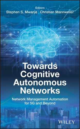
As illustrated by Figure 11.4, the profiles need to be created against a specified context, like time and/or another KPI‐like load. For dynamic KPIs that exhibit a seasonal variation, e.g. especially the traffic‐dependent KPIs, the KPI values need to be normalized against the normal daily and seasonal patterns. Then, any observed changes will be more likely to be due to the configuration change and not part of the normal fluctuation of the KPI. Time dependence may also consider a different context for each period, e.g. for each hour of day and perhaps separately for weekdays, weekends, and public holidays [10].
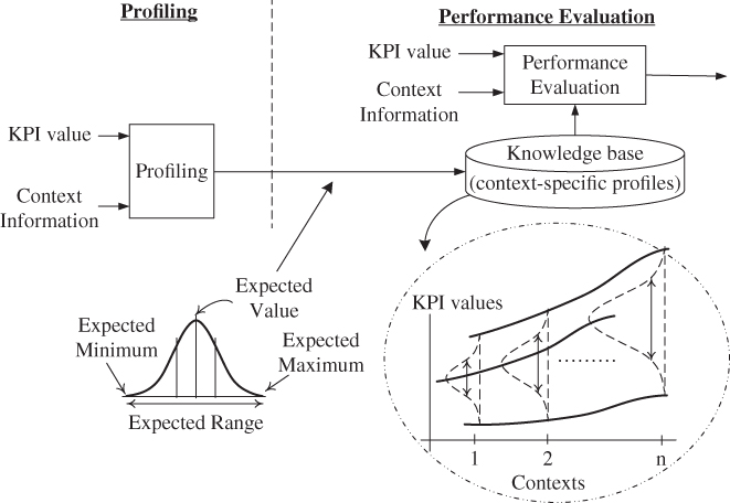
Figure 11.4 Generation and use of dynamic (context‐dependent) KPI profiles.
Using other KPIs as context implies profiling and monitoring the correlation between the monitored KPI and the context KPI. The dynamic profile will then track the profile characteristics (e.g. the expected minimum, maximum, mean …) against the different contexts as shown in the inset of Figure 11.4. For example, considering the Call Drop Rate (CDR) against load as context, the profile could state that: the target range of the CDR should be (1%, 3%) in low‐load scenarios, but that as the load increases, the two thresholds gradually increase to some maxima (e.g. [4%, 8%] respectively).
11.3.3 Degradation Detection, Scoring and Diagnosis
For the verification decision, the normalized KPI levels are typically aggregated to higher level performance indicators, to which the verification thresholds are applied. First the KPI‐level anomaly profiles are calculated and then aggregated on cell‐level, to give a cell‐level verification performance indicator. These can be further aggregated to give a similar measure for the whole verification area [10].
Similarly, instead of simply defining one so‐called ‘super KPI’ to represent the performance of the verification area, indicators may be aggregated for different performance measures, such as availability, accessibility, retainability, quality of service, mobility, etc. These may also be combined with a set of rules of what is acceptable performance level or performance change. The accuracy and reliability of the detection can also be improved by: (i) applying a hysteresis function instead of a single value and (ii) applying a Time‐to‐trigger, in which case, the detector raises/seizes an alarm only if the Super‐KPI value is above/below the detection threshold for a certain time equivalent to the specified time‐to‐trigger value.
Together with the change in the performance, the verification decision also needs to consider the context, especially the performance of the cell before the CM change. For example, different levels of freedom should be accorded to a CM change intended to optimize a stable, functioning network vs the CM change to repair an already degraded cell − more freedom should be accorded when the verification area is already in an unstable or a degraded state [10,12].
Figure 11.5 shows an example SON verification scoring function, which accounts for both the assessment score from the verification degradation process (the absolute change in performance) as well as the change in the cell's performance compared to other similar cells. For well‐performing cells, only changes that clearly improve the performance are accepted, whereas for worse performing cells more flexibility may be given in the grey and yellow zones [10].
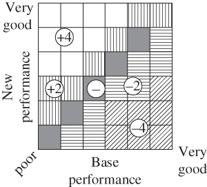
Figure 11.5 Verification assessment scoring function.
Beyond simply detecting the degradation, it is necessary to diagnose that the degradation was really caused by the CM change. For example, it may be that the reconfiguration was done to prepare for some changes in the network function's environment and that, without the change, the degradation would have been even worse. So, undoing the changes would make the situation only worse.
As discussed in Chapter 9, diagnosis is a complicated problem and it is often not possible to have a reliable diagnosis. For this reason, the verification function tries to minimize the impact of external changes in the as‐above‐described high‐level KPIs that are used in the verification decision. The simple assumption is often that after this process, all the observed changes in the performance (by comparing performance before and after the CM change) are caused by the re‐configuration. This assumption may potentially lead to false positive rollback decisions, but the deployment of the undo operations should be done in as non‐intrusive a way as possible. However, if one plans to learn from the verification decisions and to block rejected configuration changes, the impact of a false negative verification decision becomes more significant.
The diagnosis process can be improved by incorporating other known facts into the decision, e.g. the relevant (severe) alarms and the Cell status information (e.g. administrative lock). This allows the differentiation between causes and thus to take different decisions besides just ‘undo’ for each cause, e.g. to simply do nothing. However, further advanced diagnosis methods, such as those described in Chapters 9 and 10 may also be incorporated into the SON verification process.
11.3.4 Deploying Corrective Actions – The Deployment Plan
When the SON verification function has detected a degradation and has determined that it has been likely caused by the configuration change, the next step is to decide and create a plan of action regarding how the degradation could be corrected. In a simple scenario, the verification function can simply trigger a CM undo to roll the changes back and then, considering the rollback as another CM change, it re‐executes the verification process for that change. The re‐verification is necessary because the rollback may degrade the performance more than the initial CM change, for example, in case the environment of the verified network function has changed, in which case, it may be better to re‐introduce the initial CM changes [5,8,9].
Automation functions may require multiple cycles to reach their optimization goals, each cycle requiring long observation windows to monitor the impacts of each step. So, several function instances may run in parallel, each optimizing the network according to its objectives. Correspondingly, several verification operations may run in parallel, possibly with overlapping verification areas and observation windows which results in verification collisions as depicted in Figure 11.6 [13,14].

Figure 11.6 An example of a verification collision.
In a verification collision, if a degradation is detected in a cell that is included in more than one such verification areas, it is often not possible for the verification function to determine which CM change led to the degradation. For example, consider the five cells in Figure 11.6 where three cells (cells 1, 3, and 5) have been reconfigured and two (cells 2 and 5) have degraded after the CM changes. Configuring the verification areas to include the reconfigured target cell and its neighbour cells, leads to the verification areas labelled 1, 3, and 5 (respective to the target cells). However, this knowledge is inadequate to determine which change led to the degradation in cells 2 and 5.
An appropriate rollback mechanism is required for which two options are possible – an aggressive or a sequential mechanism, as described here.
- Aggressive rollback: The aggressive rollback approach would be to undo the CM changes in all three re‐configured cells 1, 3, and 5. Reasoning for such an approach could be that it would be the fastest and most certain way to return the network to a previously stable non‐degraded state. However, it is often not that simple. A rollback is a further change in the network and not without a risk of its own. There is always the risk that the rollback may make things even worse. The more changes undertaken at once, in this case undo, the higher the chance. Furthermore, as with any changes, the more parallel changes there are, the harder it is to diagnose the one that caused the degradation if one occurs. Also, since there can be many overlapping verification areas, overlapping only partially in verification areas and observation windows (time), it may be that the combined undo scope becomes very wide. As such, it is critical to undo only the changes that are most likely to have caused the degradation.
- Sequential deployment of undo actions: The other extreme would be to deploy all undo operations sequentially, i.e. one by one. However, this would also be very inefficient in a network, where there are frequent CM changes. The verification function may not be able to keep up and would become a bottleneck.
It is rarely the case that all verification areas are at verification collision with each other simultaneously. Therefore, it is possible to form an undo operation deployment plan, where only verification areas that are not in collision together are rolled back simultaneously. Figure 11.7 depicts the process of forming the undo operation deployment plan. The example shows a network of 12 cells, with their corresponding adjacency graph, in which cells 4, 7, and 10 are reconfigured. In each case, each of the verification areas v1, v2, and v3 consists of the reconfigured cell and its first‐degree neighbours. A verification collision graph is constructed with the edges connecting the colliding verification areas, in this case only areas v1 and v2.

Figure 11.7 An example of the CM undo scheduling approach.
Source: Adapted from [13].
A Graph‐colouring algorithm is applied to the verification collision graph, where each node of the graph is assigned a colour in such a way that no connected nodes share the same colour. The undo deployment plan is then formed so that only verification areas of a certain colour are deployed simultaneously and thus avoiding simultaneous undo actions amongst colliding verification areas [13].
The undo operations can be prioritized, for example, so that the colour containing the verification areas with the highest total number of degraded cells are always rolled back first. On using this rule for the example in Figure 11.7, verification areas v1 and v3 would be undone first. Then, v2 is rolled back in the subsequent correction window, but only in case the undo of the change in cell 4 has not already corrected the degradation [13].
11.3.5 Resolving False Verification Collisions
Deploying an undo operation can be a time‐consuming task since the impact of the undo also needs to be verified. In a network with lots of reconfigurations there might be insufficient correction timeslots available for deploying the corrective actions even utilizing the graph‐colouring approach described in the previous subsection. Therefore, it is desirable to detect the verification collisions that could be resolved before deploying the corrective actions [14].
Figure 11.8 shows a false verification collision in a network of 10 cells. Cells 1, 2, and 3 are reconfigured leading to the depicted verification areas, as identified by the respective target cell. Now, consider that cells 5, 8, and 9 are degraded and that the verification mechanism is unaware that cell 2 is not responsible for any of the degradation. Since the degraded cell number 8 is included in all three verification areas, three correction deployment slots are required for the undo operation. However, since cell 2 isn't causing any degradation, the collision between verification area 2 and verification areas 1 and 3 are false verification collisions.
Figure 11.8 Example of a verification collision [14].
One approach for resolving such false verification collisions is by employing a behavioural graph, which indicates the degree of similarity amongst the performance in several cells. To demonstrate its usage, consider the example shown in Figure 11.9 with two KPIs a1 and a2 as the features to be used in the verification process. With the anomaly level of the features as the dimensions of the graph (see step 4), each cell is placed on the graph according to its anomaly levels for the respective features. For simplicity, some cells are completely overlapping in this example as indicated by the numbers in the graph vertices (e.g. cells 5, 9, and 12 at vertex V5,9,12).
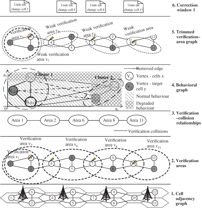
Figure 11.9 An approach for detecting false verification collisions [14].
A fully connected graph is constructed amongst all the cells, with the weight of each edge as the Euclidian distance between the cells on the feature map. Then, removing a configured number of longest edges or edges longer than a set maximum edge‐weight, the behaviour graph is transformed into an anomaly graph that clusters similarly performing cells together.
The result that cells belonging to a certain cluster exhibit similar anomalous behaviour in the verification process can be utilized to try to detect false verification collisions. Collisions between weak verification areas are eliminated by removing those extended‐target‐set cells from the verification area, which do not belong to the same cluster with the target cell of that verification area. For example, removing the edge (V3,7 − V6,11) indicates that cells 6 and 7 do not need to be in the same verification area, so cell 7 is removed from verification area V6 creating the smaller ‘weak verification area 6’ shown in step 5. This process eliminates the weak collisions between the verification areas allowing multiple simultaneous undo actions to be deployed.
In the example, the process results in a requirement for only two correction windows for the four verification collisions, i.e. only verification areas 1 and 2 in Figure 11.9 overlap necessitating separate two windows. The other areas can be deployed concurrently to verification area 1 in correction window 1.
The combination of the above processes ensures that network automation functions can be supervised to ensure that only their positive influences are accepted to the network and any negative influences addressed through these undo operations. The verification concepts, although developed for the SON framework, expect to be usable even when the functions are cognitive since they provide means of redress or at least a feedback mechanism to the cognitive function to re‐evaluate their actions and minimize negative influences. The next section shows one such usage of the verification concept.
11.4 Optimistic Concurrency Control Using Verification
A major requirement for NMA systems is concurrency control, i.e. ensuring that network performance is not degraded because of multiple automation functions acting concurrently on the network. The simplest response in the SON paradigm has been to apply SON coordination mechanisms as the solution. Therein, the safest SON coordination scheme executes only one SON function instance at a time in the whole managed network, but this would be very inefficient. Another approach is to only allow SON functions with non‐overlapping impact areas and times to run at the same time. Although more efficient than network‐wide serialization, this approach also restricts the number of active SON function instances significantly, especially due to the long impact times of many SON functions. The execution of one function can last for several granularity periods (GPs) (the smallest periods of data collection) and the result can be the same function requesting to execute again. On the other hand, it is imperative that conflicts between SON function instances can be avoided. A combination of pre‐ and post‐action coordination, namely combining SON coordination and SON verification, can be used to optimize the coordination performance and to implement an optimistic concurrency control (OCC) strategy [9].
11.4.1 Optimistic Concurrency Control in Distributed Systems
OCC assumes that multiple transactions can often complete without interfering with each other [15], so running transactions use data resources without locking the resources. Before committing, each transaction verifies that no other transaction has modified the data it has read. In case of conflicting modifications, the committing transaction rolls back and can be restarted. In systems, where the data contention is low, this offers better performance, since managing locking mechanisms is not needed and excessive serialization can be avoided [16].
In performance‐critical distributed applications, data is additionally often processed in batches, to avoid the performance penalties of numerous remote procedure calls. When OCC is used, parallel batch operations are not synchronized, and this can lead to race conditions between some data elements in the batches. Database constraints, for example, can be used to check the consistency of the stored data and to catch such conflicts. In case of a constraint violation, the transaction for the whole batch is rolled back. The operation is then retried by the application with stricter concurrency control and possibly one by one for each of the batch elements. Using this method, performance remains good, when most of the batch write operations are successful and conflicts are rare but, at the same time, it ensures that one invalid element does not prevent processing the whole batch.
11.4.2 Optimistic Concurrency Control in SON Coordination
Figure 11.10 highlights how OCC can be implemented with the SON coordination and verification concepts. The basic idea is that the SON coordinator can allow for more parallel execution of SON function instances, if the result of the optimization actions taken by the functions is verified by the SON verification function. SON verification will ensure that any possible degradations that are a result of the conflicts are quickly resolved. This can be further optimized by changing the SON coordination policy based on the verification results. In case verification detects a degradation, the SON coordinator switches to a stricter coordination policy in the specific verification area. It can, for example, completely serialize the SON function instance execution until all functions have run at least once, after which the original more parallelized SON coordination scheme can be continued [16].

Figure 11.10 Optimistic concurrency control using SON coordinator and verification.
A more complicated organization of the Functions could also be considered when SON verification is combined to the coordination mechanism. For example, the conflicting SON function instances may from the SON‐coordination perspective be placed into two categories: the hard conflicts, which must never be run in parallel and the soft conflicts, i.e. coupled function instances, which can only be run in parallel if the outcome is verified by SON verification. Correspondingly, the coupled instances can mostly be run simultaneously with the expectation of some infrequent race conditions.
11.4.3 Extending the Coordination Transaction with Verification
To enable this opportunistic concurrency control mechanism, the coordination transactions need to be extended with SON verification as depicted in Figure 11.11. When a SON function instance wants to optimize certain Network parameters, it sends an execution request to the SON coordinator which then initiates a new coordination transaction. Through this transaction, the coordinator coordinates the CM changes in the transaction area which includes all the Network Functions that are within the impact area of the SON function instance [16].

Figure 11.11 The extended SON coordination transaction implementing OCC.
In [1,17,18], the coordinator had only two decisions – either acknowledge (ACK) or reject (NACK). Extending these concepts, a third decision is now added. With an ACK decision, the network automation function instance is allowed to provision its CM changes in the network and the transaction ends (commit). Here, the coordinator does not require the changes to be verified, but they may be independently verified depending on the system configuration and the operator policies. For the NACK decision on the other hand, the SON function instance is not allowed to provision its CM changes in the network and the transaction ends. Opportunistic concurrency control introduces the Acknowledge with Verification (ACKV) decision, where the SON function instance is allowed to provision its CM changes in the network, but the coordinator keeps the transaction open and marks it for verification. The ACKV decision is signalled to the verification with at least three information elements, i.e.: (i) Transaction area, (ii) the originating SON function instance, and (iii) the updated CM parameters (see Figure 11.11a).
Verification wraps the coordination transaction in a higher‐level verification transaction, which in the case of parallel verification requests with overlapping transaction areas may contain several coordination transactions. If the verification function is not able to verify the changes, for example, due to conflicting ongoing verification operation, it will reject the request for verification and the transaction must be rejected. Alternatively, the SON coordinator can execute batch coordination for the transactions, to check if some of the requests can still be acknowledged.
If the transaction area of the coordination transaction overlaps with another ongoing verification operation, the verification mechanism must decide, if the coordination transaction can be added to the existing verification transaction. Otherwise, it must be rejected, and the coordinator must be notified about the rejection.
As in [9], at each granularity period (GP), the verification monitors the KPIs and decides for each verification transaction either to ‘pass’, ‘undo’, or ‘continue monitoring’. A ‘Pass’ implies that all coordination transactions with their CM changes contained in the verification transaction are acknowledged and closed. An ‘Undo’ implies that all the coordination transactions contained in the verification transaction are rejected, their CM changes are rolled back, and the transactions are closed. Finally, a ‘Continue monitoring’ decision implies that the SON verification mechanism will monitor the verification area performance for at least one more GP and that the verification transaction and all contained coordination transactions remain open during this period.
The open challenge then is how to group requests into either ACK, NACK, or ACKV. This can be statically configured, i.e. according to the network automation function models provided by the function vendor. The coordinator may, for example, statically decide that conflicts between specified SON functions would not lead to acknowledging one and rejecting the other, but both would be acknowledged with verification. However, such a static approach can lead to situations where the function instances get caught in a conflict causing degradation, and a rollback by the SON verification mechanism, only to restart the same cycle from beginning.
The principles of OCC avoid rollback loops through an opportunistic coordinator. As before, the coordinator acknowledges requests with verification whenever possible instead of rejecting them. However, if verification rejects a coordination transaction, the coordinator switches into strict concurrency control in the specific transaction area, i.e. allowing only one function instance to run at a time or only function instances that are known not to conflict with each other, as in [18,19]. Strict concurrency control continues until all automation function instances have run at least once or until a pre‐configured time threshold is reached, after which, the coordinator reverts to relaxed concurrency control. This allows the function instances to reach their targets without conflicts from race conditions.
11.5 A Framework for Cognitive Automation in Networks
As has been discussed in Section 11.1, SON is unable to autonomously adapt to complex and volatile network environments, e.g. due to frequently changing operating points resulting from high cell‐density as in UDNs, virtualization and network slicing in 5G RANs [20], or from frequently changing services/applications requirements and characteristics. The solution to this challenge is the use of Cognition in Network Management, i.e. the use of Cognitive Functions as the intelligent OAM functions that can automatically modify their state machines through learning algorithms [21]. Correspondingly, in the CAN paradigm, these complex multi‐RAT, multi‐layer, multi‐service networks shall remain operable with high (cost) efficiency of network management and with considerably lower necessity for manual OAM tasks.
11.5.1 Leveraging CFs in the Functional Decomposition of CAN Systems
The CAN paradigm advances the use of cognition in networks to: (i) infer environment states instead of just reading KPIs and (ii) allow for adaptive selection and changes of NCPs depending on previous actions and operator goals. The general idea, for example, in [21,22], is that CFs will: (i) use data analytics and unsupervised learning techniques to abstract, contextualize, and learn their environment, and then, (ii) use Reinforcement Learning (RL) techniques like Q‐learning to either learn the effects of their actions within the specific defined or learned contexts [21,22] or simply to learn how to act in such environmental contexts. The design of the CAN system needs to take advantage of the CFs' capabilities not only to account for the behaviour of each CF both individually and collaboratively besides other CFs but also to allow for flexible deployments – be in centralized, distributed, or hybrid scenarios.
The proposed blueprint for the CAN system decomposes the system into smaller inter‐related functions that leverage cognition at each step/function. The design leverages ‘active testing’ benefits that are inherent in machine learning (ML), i.e. knowledge build‐up requires CFs to execute unknown configurations and evaluate how good or bad they perform in each context, which is the central feature of ‘active testing’.
The proposed CF framework comprises five major components as shown in Figure 11.12 [29]: the Network Objectives Manager (NOM), the Environment Modelling and Abstraction (EMA), the Configuration Management Engine (CME), the Decision Applications (DApps), and the Coordination Engine (CE). These components include all the functionality required by a CF to learn and improve from previous actions, as well as to learn and interpret its environment and the operator's goals. While the CF operates in the same environment as SON functions, it deals differently with the KPIs' limited representation of the environment. Instead of simply matching network configurations to observed KPIs, the CF infers its context from the combination of KPIs and other information (like counters, timers, alarms, the prevailing network configuration, and the set of operator objectives) to adjust its behaviour in line with the inferences and goals. The subsequent sections describe the roles and interworking of the five CF components. Note that the discussion here is independent of the component implementation architecture. i.e. Figure 11.12 only depicts the required interfacing be it in a centralized, distributed, or hybrid implementation.
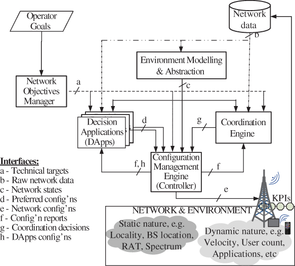
Figure 11.12 CAN framework – Functions of CAN system and related cognitive functions. [29]
11.5.2 Network Objectives and Context
The generic input to the system is provided by the NOM and EMA, which respectively provide the operator or service context and the network environment and performance context.
The NOM interprets operator service and application goals for the CAN or the specific CF to ensure that the CF adjusts its behaviour in line with those goals. The other components take this interpretation as input and accordingly adjust their internal processes and subsequently their behaviour. In principle, each CF needs to be configured with the desired KPI targets and their relative importance, which the CF attempts to achieve by learning the effects of different NCP values. Without the NOM, such targets would be manually set by the operator who analyses the service and application goals (or KQIs) to derive the network KPI targets and their relative priorities. In this design, the NOM replaces this manual operation by using cognitive algorithms to break down the input KQIs (which are at a higher level of abstraction) into the output which are the prioritized KPI targets at a lower abstraction level.
The EMA on the other hand abstracts measurements into environment states which are used for subsequent decision making. Such environment abstractions (or ‘external states’) that represent different contexts in which the CF operates are built from different combinations of quantitative KPIs, abstract (semantic) state labels, and operational scenarios like the prevailing network or function configurations. Note that although SON also uses KPIs and current network configurations in the decision, it does not make further inference about the environment but instead responds directly and only to the observed KPIs. Even where contexts may be abstracted, the set of possible external states (usually, the considered KPIs) is fixed since it must be accounted for in the algorithm rules and the underlying decision matrix. The CF uses the EMA module to create new or change (modify, split, delete, etc.) existing quantitative or abstract external states as and when needed. These abstract states are then used by the further CF sub‐functions – the DApp and CME, which may optionally also individually specify the KPIs, the level of abstraction, the frequency of updates, etc. that they require.
The simplest EMA engine is an ML classifier that clusters KPIs or combinations thereof into logically distinguishable sets. Such a classifier could apply a Neural Network, a Support Vector Machine (SVM), or similar learning algorithms to mine through KPI history and mark out logical groupings of the KPIs. Each group represents one environmental abstraction – requiring a specific configuration. Note, however, that an advanced version of the EMA may add an RL agent that selects the appropriate abstractions and (preferably) reclassifies them for the specific CF.
A centralized EMA provides the advantage of working with a wider dataset (network performance measurements, KPIs, context, etc.) across multiple cells or the entire network. While individual CFs can only have a limited view of the network context, a centralized EMA collects data across a defined network domain. This does not mean that it provides KPIs with the same level of abstraction to all CFs. Rather, depending on the CF and its feedback on the KPIs and context, the EMA dynamically adapts/changes its output. This will generally include multiple scales of measure, e.g. from ratio‐scale KPIs to interval‐scale metrics and to semantically enriched nominal‐scale state descriptions. Further, the level of precision and accuracy can be modified dynamically.
11.5.3 Decision Applications (DApps)
The DApp matches the current abstract state (as derived by the EMA module) to the appropriate network configuration (‘active configuration’) selected from the set of legal/acceptable candidate network configurations. The DApp has the logic to search through or reason over the candidate network configurations, and to select the one that maximizes the probability of achieving the CF's set objectives for that context. In the SON paradigm, such an engine was the core of the SON function and the network configurations were selected based on a predefined set of static rules or policies (the decision matrix in Figure 11.1). In a CF, such an engine will learn (i) the quality of different network configurations, (ii) in different contexts (as defined by the EMA), (iii) from the application of the different legal network configurations, and (iv) towards different operator business and service models and associated KQIs. It will then select the best network configuration for the different network contexts, making the mapping (matching abstract state to network configuration) more dynamic and adaptive.
For this, the internal state space and state transition logic of the DApp (replacing the SON function's decision matrix) must also be flexible. Since there are no rules here (to be changed), changes in the DApp internal states (and transitions) are triggered through the learning. For example, using a neural network for selecting configurations, the DApp may be considered as a set of neurons with connections amongst them, in which neurons fire and activate connections depending on the context and objectives.
Besides the examples in Chapters 7–10, there are multiple ways in which the DApp may be implemented, typically as supervised learning or RL agents. The neural network example above could be an example instantiation of the supervised learning agent which is trained using historical network statistics data. It then employs the learned structure to decide how to behave in new scenarios. Using RL, the DApp could be a single‐objective RL agent that learns the best network configurations for specific abstract states and CF requirements. The single objective hereby is optimizing the CF's requirements which may, in fact. consist of multiple targets for different technical objectives or KPIs as set by the NOM. As an example, for the MRO use case, the single objective of optimizing handover performance translates into the multiple technical objectives of minimizing radio link failures while simultaneously minimizing handover oscillations. Also, since there may not always be a specific network configuration that perfectly matches specific contexts, fuzzy logic (where truth values are not binary but continuous over the range [0,1]) may be added to RL to allow for further configuration flexibility network.
For most use cases, the DApp will be distributed (i.e. at the network function/element, like the base station) to allow for a more scalable solution even with many network elements. However, a centralized implementation is also possible either for a small number of network elements or for use cases with infrequent actions, e.g. network self‐configuration scenarios like cell‐identity management. Optionally, the CME may be integrated into the DApp, which is especially beneficial if both functions are co‐located.
11.5.4 Coordination and Control
The Cognitive NMA system requires means to control the individual functions and to coordinate amongst their behaviour. This responsibility is undertaken by two units – the Configuration Management Engine (CME) and the Coordination Engine (CE) – which may, in some implementations, be combined into one.
11.5.4.1 Configuration Management Engine (CME)
Based on the abstract states as inferred by the EMA module, the CME defines and refines the legal candidate network configurations for the different contexts of the CF. In the simplest form, the CME masks a subset of the possible network configurations as being unnecessary (or unreachable) within a specific abstract state. In that case, the set of possible network configurations is fixed, and the CF only selects from within this fixed set when in the specific abstract state. However, a more cognitive CME could also add, remove or modify (e.g. split or combine) the network configurations based on the learning of how or if the network configurations are useful.
The CME is a multi‐input multi‐objective ML agent that gets input from the EMA and CE to determine the set of legal configuration candidates, i.e. the active configuration set. It learns the set of configurations that ensure accurate/effective fast‐to‐compute solutions for the CF's objective(s), the operator's objectives, and the CE requirements/commands. The simplest CME is a supervised ML agent (applying a Neural Network, an SVM or similar algorithm) that evaluates historical data about the quality of the configurations in different contexts (environmental states, peer functions, etc.) to select the legal configurations. However, an online ML CME could apply reinforcement learning to continuously re‐adjust the legal set as different configurations are applied and their performance evaluated.
A centralized CME manages the internal state space for all CFs by constantly monitoring and updating (i.e. modifies, splits, deletes, etc.) the set of legal configurations available for each CF. Again, the advantage here consists of taking more informed decisions due to a broader dataset and sharing state‐space modelling knowledge across multiple CFs. However, to manage scalability, e.g. for the case where multiple different CFs are implemented, a feasible centralized CME (and the most likely implementation) will only manage network configuration sets for CFs and not for CF instances. In that case, final NCP selection will be left to the DApp decisions/learning of each instance.
11.5.4.2 Coordination Engine (CE)
Like SON, the CNM paradigm also requires a coordination function, albeit of a different kind. Since the CFs will be learning, the CE needs to differently coordinate the CFs whose behaviour is non‐deterministic owing to the learning. Specifically, the CE detects and resolves any possible conflicting network configurations as set by the different CFs. Additionally, (for selected cases) it defines the rules for ‘fast track’ peer‐to‐peer coordination amongst CFs, i.e. it allows some CFs to bypass its coordination but sets the rules for such by‐pass actions. It also enables cross‐domain knowledge and information sharing (i.e. across different vendor/network/operator domains). This may include environment and network models as well as the relevance and performance of KPIs and CF configurations in different contexts. Moreover, it supports the EMA and CME by identifying CFs with similar context in environment and legal configuration sets.
As stated earlier, the CE needs to (i) learn the effects of different CF decisions on other CFs; (ii) interpret the learned knowledge; and (iii) optionally suggest modifications to the CME and DApp on how to minimize these effects. Thereby, it undertakes the supervisory function over the CME and DApp, e.g. it may request the CME to re‐optimize the legal configurations list but may also directly grade the DApp actions to enable the DApp to learn configurations that have minimal effects on other CFs.
If deployed in a distributed manner (i.e. at the network function), the CE becomes a member of a MAS of learning agents, where each agent learns if and how much the actions of its associated DApp affect other CFs or CF instances. It then appropriately instructs the DApp to act in a way that minimizes these negative effects. For this, the CE instances would have to communicate such effects with one another as suggested in [22,23]. Otherwise, in a centralized CNM approach, the CE is also centralized to allow for a multi‐CF view in aligning the behaviour of the CFs.
11.5.5 Interfacing Among Functions
The individual CF components described above interact via the interfaces depicted in Figure 11.12. Interface a from the NOM towards the CE, CME, and DApp is used to convey the KPI targets to each CF. The latter three components then read raw network state information like KPIs over interface b, and also receive individually customized representations of the current environment from the EMA component via interface c. A configuration change proposal computed by any of the DApps is transmitted to the CME for implementation via interface d while the CME activates via interface e. The activated network configurations are reported by the CME to the DApps and CE via interface f, which may also be extended to the EMA if the EMA's descriptions of the environment states also include the active network configuration values. The CE uses interface g to convey information on the impact of a CF's NCPs to the CME, e.g. by notifying which NCPs (or values thereof) have shown an adverse effect on the objectives of other CFs. Finally, interface h is used by the CME to update the set of legal configurations of the DApps. Further details on the information content of these interfaces are given in Table 11.1.
Table 11.1 Descriptions of the required interfaces between CF component blocks.
| Type | From | To | Information provided | Remarks |
| a | NOM | CE CME DApps |
KPI target (values) to be achieved by the CFs Optional: target interpretations to distinguish their respective relevance; weights, priorities or utilities of the different KPIs |
KPI targets may be universally sent to all so that each entity filters out its functionally relevant targets, or differentiated per recipient, e.g. the CME and DApp get only CF specific targets, CE gets the targets for all CFs. |
| b | Network, OAM, … | EMA | Current network state parameter and KPI values | Allows DApps, CME and CE to evaluate how good certain actions are for the CF at hand, requiring |
| c | EMA | CE, CME DApps |
Abstract environment states or contexts as created by the EMA. | States may be generic or specific to each CF, provided they have a common reference. But recipients may also specify the abstraction level required for their operation. |
| d | DApps | CME | Proposed network (re)configurations; Reports on the quality of the action(s) per context | May also be implemented directly between DApps to exchange reports on actions taken |
| e | CME | network | Activation of selected and approved network configuration values | |
| f | CME | CE, EMA, DApps | Reports on CME's network configurations and quality of the action(s) per context | Optional for the EMA: needed only if its state abstraction includes current configurations |
| g | CE | CME | CE configuration or report for each CF Simple: description of effects of CF action Optional: CE decisions/recommendations/ |
The CME uses the input to (re)configure the CF's control‐parameter spaces. Recommendations/decisions may e.g. specify actions that should never be re‐used |
| h | CME | DApps | KPI report on the DApp's action(s), CME configuration of the CF's action space (set of legal network configurations) | If the configurations database is part of the DApp, such configurations are sent to the DApps. Otherwise, the CME independently edits the standalone database. |
11.6 Synchronized Cooperative Learning in CANs
The CAN framework successfully justifies the use of ML for developing Cognitive Functions. More especially, using RL, each CF can learn the optimal to behave for all possible states in a particular environment. The assumption here is that the CF is afforded an environment to learn the independent effects of its actions and to determine the best actions to apply in a given state. However, even when acting alone, CFs can affect each other's metrics. For example, an MLB‐triggered Cell Individual Offset (CIO) change in a cell can affect MRO metrics right after the change and at later points in time. Synchronous separation of the function execution (be it time or space) can thus not solve the challenge in this case, yet a coordinator would be too complex for learning‐based CFs since it must account for the non‐deterministic nature of the CFs. A good alternative in this case is SCL where the complex coordinator is replaced by an implicit mechanism that allows the CFs to communicate their effects to one another as described here.
11.6.1 The SCL Principle
Consider a network with C cells where each has F CF instances (also herein referred to as the learning agents) indexed as CFi ∀ i ∈ [1, f]. If, in a particular network state CF instance i in cell j (CFji) takes an action, that action will affect peers CFjl ∀ l ∈ [1, f]; l ≠ iwhich are the other CFs in cell j as well as the peers CFci ∀ c ∈ [1, k]; c ≠ j & ∀ i ∈ [1, f], which are all the CFs in the other cells. For optimal network‐wide performance in that state, CFji needs to act in a way that its action has: (i) the best performance considering CFji′s metrics and (ii) the least effects on the peers. Thereby, CFji needs to know the likely effects of its actions on the peers which requires that it must learn not only over its metrics but also over those peer effects.
The SCL concept enables this learning across multiple CF metrics through the three‐step process illustrated in Figure 11.13, which involves:
- After executing an action, CFji informs all its peers about that action triggering them to initiate measurements on their performance metrics.
- At the end of a specified monitoring period which may either be preset and fixed or may be communicated as part of step 1, the peers report their observed effects to the initiating CF (here CFji).
- The initiating CF (CFji) then aggregates the effects across all the reporting peers and uses that aggregate to evaluate the quality of its action and update its learned policy function.
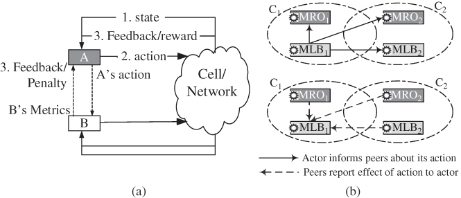
Figure 11.13 Synchronized cooperative learning: (a) the SCL concept for two cognitive functions and (b) example message exchanges in two cells.
In Figure 11.13a, for example, A informs B whenever it (A) takes an action, prompting B to monitor its metrics. At the end of the observation period, B informs A of the corresponding effects on B's metrics, with which A derives a penalty that qualifies the action. If the action was acceptable or good to B, A may not penalize that action in a way encouraging the action to be reused in future. Otherwise A may heavily penalize the action to ensure it is blacklisted.
In a scenario with multiple CF instances, each CF instance that receives the active CF's message must report its observed effect, so that the reward/penalty is derived from an aggregation of all of the reports. For example, for the two cells in Figure 11.13b, both with instances of MLB and MRO, after taking an action in C1, MLB1 the MLB instance in cell C1, receives responses from MRO instances in both cells C1 and C2 as well as from the MLB instance in cell C2.
With the possibility of having multiple cells either as actors or as peers, two challenges must be addressed to guarantee optimal results:
- How to manage concurrency amongst CF instances within or across cell boundaries.
- How to aggregate the received information in a way that ensures effective learning.
These are described in the subsequent sections as are ideas on how to address them.
11.6.2 Managing Concurrency: Spatial‐Temporal Scheduling (STS)
After CFji has taken an action, for it to receive an accurate report from a peer CFcl, it is important that during the observation interval, CFcl's metrics are not affected by any other agent except CFji. Otherwise, since CFcl is not able to differentiate actions from multiple CFs or instances thereof, its report will be misleading. It is appropriate to assume that CFji only affects CF instances in its cell or those in its first‐tier neighbour cells and not in any other cells further out. This is a justified assumption except for a few radio‐propagation‐related automation functions, like interference management, which can easily be affected by the propagation of the radio signal beyond the first‐tier neighbour cells. Even then, compared to effects in first‐tier neighbour cells, effects in second and higher‐tier neighbours are typically so small that they can be neglected.
Correspondingly, the assumption of having effects only in the cell and its first‐tier neighbours and the requirement that CFcl is only affected by CFji (at least during learning), imply that, CFs should only be scheduled so that no two CFs concurrently affect the same space‐time coordinate, especially during the learning phase. This resulting mechanism, called Spatial‐Temporal Scheduling ensures that each metric measurement scope (a space for a given time) is affected by only one CF, i.e. CFs are scheduled in a way that each CF acts alone in a chosen space‐time coordinate.
For the learning‐time spatial scheduling, consider the subnetwork of Figure 11.14 and a CF A with an instance executed in cell 14 (i.e. A14). For A14 to learn the independent effects of its actions on the critical peers – CFs in 14 and its tier 1 neighbours (e.g. 12, 16), it is necessary that during A14's observation interval:
- only A14 is executed in cell A and no CF is executed in any of the neighbour cells to cell 14, otherwise, effects observed in cell 14 would not be unique to A14.
- No CF is executed in any of cell 14's tier‐2 neighbours (e.g. 23, 15), otherwise, the effects in cell 14's tier‐1 neighbours (e.g. in 12, 16) would not be unique to A14.

Figure 11.14 Spatial cell scheduling for concurrent actions in a hexagonal‐grid.
This implies that the nearest concurrent action to A14 should be in cell 14's tier‐3 neighbours (e.g. cell 10), which are outside A14's reporting area. The result is the reuse‐7 clustering profile of Figure 11.14 where concurrent activity is only allowed within a Cluster/set of cells with the same colour in the Figure 11.14. By doing this, each CF can measure its effects on the critical CFs without influence from any action in the potential conflict cells and CFs. To achieve this, SCL applies the time division multi‐frame of Figure 11.15 with 7‐frames per multi‐frame which ensures that each of the seven clusters gets 1 frame of the 7‐frame multi‐frame.
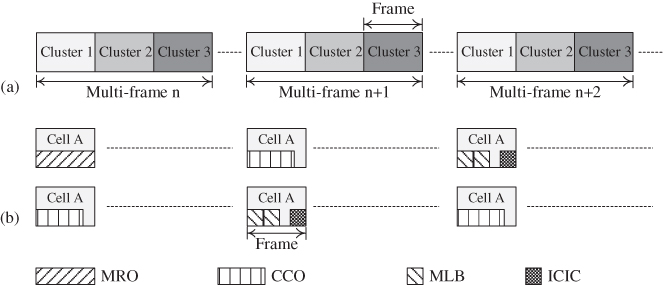
Figure 11.15 Space and Time separation of CF execution: (a) Cluster Frames in a Multi‐frame and (b) STS scheduling in two cells during different multi‐frames.
The clustering can be configured by the reuse‐7 graph colouring scheme which allocates every one of any seven neighbour cells to a different Cluster creating the mapping illustrated by Figure 11.14. Given a seed cell, the graph‐colouring algorithm first allocates to the seed's immediate neighbours ensuring there are two cells between any two identically‐coloured cells, effectively allocating each of the seed's neighbours to a different cluster. Then, starting with any of the seed's second‐tier neighbours, the algorithm again allocates cells to clusters following the same rule, i.e. ensuring there are two cells between any two identically‐coloured cells.
11.6.3 Aggregating Peer Information
The space‐time scheduling of CFs enables the CFs to make accurate observations of their environment and give accurate reports of their observation thereof. The simplest report of the observations is the hash of the important KPIs and their values for the respective peer CFs. This minimizes the need for coordinating the design of the CFs, i.e. no prior agreement on the structure and semantics of the report is necessary although it raises the concern of different computations (thus meanings) of the KPIs. However, to understand the concepts however, it is adequate to assume that this simple reporting mechanism is used.
Given the multiple metric reports of KPI‐name to KPI‐value hashes from the different peers, for the initiating CF (CFji) to learn actions with the least effects on those peers, CFji requires an appropriate objective function for aggregating those metrics. Thereby, for each peer that sends a report, CFji requires a peer‐specific local ‘goodness model’ of the metrics i.e. a specific model that describes which metric values are good or otherwise. The model must be specific for each actor‐peer CF pair since each CF affects each peer CF in a way that is specific to the acting CF and the peer. In Figure 11.13b for example, both MRO instances report the PP and RLFs rates while the MLB in cell B reports the dissatisfied user rate over the measurement interval, so the initiating CF (MLB1) must account for the MRO effects different from the MLB effects when deriving the associated quality of the action taken.
Moreover, the initiating CF may also require an effect model for the different peers to describe the extent to which it should account for a given peer's observations. This model, which will typically be different for different CF instances would, for example, differentiate peers in the same cell as the initiator CF from those in neighbouring cells. For the MRO‐MLB case, for example, the MRO effect model may consider neighbour cells' MLB effects as being insignificant, yet the MLB effect‐model may consider neighbour cells' MRO effects as critical to the performance evaluation.CFji must then use the combination of goodness and effect models to evaluate the aggregate effect of its actions on the peers. Ideally, this will translate into a generic operator‐policy aggregation function, typically as a weighted multi‐objective optimization function, for which the operator sets the weights.
11.6.4 SCL for MRO‐MLB Conflicts
The MRO‐MLB conflicts are the most widely discussed conflict in SON, so it makes sense to use that to demonstrate the SCL ideas. This assumes that the two Cognitive Functions are implemented as Reinforcement learning (Q‐learning) based agents as described in Chapter 9 (Sections 9.3 and 9.4). The characteristic behaviour of the two functions (hereafter respectively referred to as QMRO and QLB) are:
- Each CF observes a state (mobility for QMRO and load distribution for QLB).
- The CF selects and activates an action on the network (the Hys‐TTT tuple for QMRO and the CIO for QLB).
- The CF evaluates a rewards function that describes how good the action was for the network.
Considering a network of 21 cells with wraparound as in Figure 11.14, each cell is availed an instance each of QMRO and QLB. However, to improve the speed of convergence, the different instances of single CF (e.g. QMRO) learn a single‐shared policy function. The cells and CF instances are clustered by a graph‐colouring algorithm and configured with execution time slots are described in Section 11.6.2. To implement the SCL mechanism, steps 2 and 3 above are adjusted such that:
- after activating the action, the CF informs the peers of the action and requests them to evaluate their metrics for an interval that is specific to the active CF.
- The affected peer CFs report their metric values for the specified period and the initiating CF aggregates these in the reward used to evaluate the action.
The critical aspect then is how to design the rewards functions that enable each CF to learn based on the aggregate of the received information and its own measurement. As described above, the appropriate function needs to account for differences in CF types and instances. This, however, can be complex so to reduce complexity yet still evaluate SCL's benefits, the evaluations here only consider CF instances within the same cell and neglect intra‐cell effects, i.e. a single‐effect model is used with effect = 1 for intra‐site peers and effect = 0 all other CFs. Considering Figure 11.13b, for example, this mechanism implies that after its action in cell C1, MLB1 only considers the feedback from MRO1, and neglects the effects on MRO and MLB in cell C2. This may not be enough to account for all effects, but the complete aggregation function requires a detailed study that quantifies the actual cross‐effects among the CFs. The MLB and MRO reward functions are designed as described here:
11.6.4.1 QMRO Rewards
Alongside minimizing RLFs and PPs, QMRO needs to account for MRO effects on load, to minimize the Nus by, for example, reducing the load in an overloaded cell. To account for MRO effects on load, the reward derived from the Handover Aggregate Performance (HOAP) metric is scaled by a Loadbonus = 0.9 as given in Eq. (11.1), but only if the overload significantly reduces after MRO. Otherwise, the default Loadbonus = 1 is applicable.
‘Significant load change’ occurs if the cell was overloaded at the time of MRO action but the offered load subsequently reduced by more than 20%. The 20% reduction applied in all cells is heuristically obtained, but with two straightforward principles. Firstly, actions leading to load reduction will have better quality, if their respective loadbonus are less than the default. Secondly, the reward should not over emphasize load reduction to the extent that the initial MRO focus is lost, i.e. the MRO goal of minimizing RLFs and PPs should be paramount. These principles ensure that QMRO prioritizes MRO but with an eye to reducing any observed overloaded.
11.6.4.2 QLB Reward Function
To account for MRO effects while pursuing the QLB objective of instantaneously removing overload, QLB also now requires the penalization of actions that cause excessive degradation of HO performance. For each load scenario, Γ as defined in section QLB, the revised reward function adds an HO‐related penalty (HOpenalty) as in Eq. (11.2).

where Δρs is the achieved reduction in the serving cell offered load ρs and Δρn is the change in average target cells offered load. For the MLB decision, a HOcost can be estimated as in Eq. (11.3). Using this HOcost, the HO penalty can be derived from a penalty function like that in Figure 11.16.
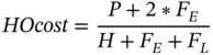
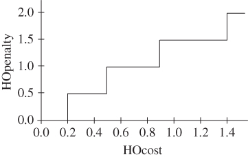
Figure 11.16 Example handover penalty function.
11.6.4.3 Performance Evaluation
Performance of SCL is evaluated by comparing: (i) to Ref the reference network without any CNM solutions but having manually optimized HO settings, (ii) to QBOTH, which is the operation of the two functions without any coordination solution (here denoted by), and (iii) STS which is the operation with only STS as an example implementation of Single Agent Systems decomposition solution. In all cases, two perspectives are considered:
- Transient performance: With gains as the percent reductions in HOAP and Nus for each batch relative to Ref, the transient results track the Simple Moving Average (SMA) of the gains in each metric using a window of 10 values (i.e. 10 batches). For example, if at t = τ the Ref and SCL Nus are respectively
 and
and  , the transient Nus is
(11.4)
, the transient Nus is
(11.4)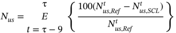
- Steady state performance: In the results, all solutions complete learning between 20 000 and 30 000 s. So, steady‐state performance plots on a 2D grid the metric averages for the last 20 batches (which are all after 30 000 s). Note that Nus here indicates the average number of dissatisfied events per second evaluated over the measurement period (e.g. a batch) in the network.
11.6.4.4 Observed Performance
The performance of SCL can be summarized by Figure 11.17 which evaluates the transient performance in terms of the HOAP metric [22] and the number of dissatisfied users (Nus). It is visible from the Figure 11.17 that compared to QBOTH, SCL achieves good compromise between the two CFs, although may not always be better than STS. During learning, SCL and STS performance is equivalent since the same CFs are active and exploring in the same way. After learning is completed, however, the performance differs because the learned policy functions are different. For SCL, each CF is not only given a chance to learn its independent policy function but is also required to learn the solutions that have minimal effect on the peers. The cooperative competition minimizes trigger oscillations, i.e. CFs need not be triggered in response to a peer's action since the peer ensures that its actions have minimal negative effects on other CFs.

Figure 11.17 Transient performance of SCL‐based CF coordination in a network with a 50 m wide hot‐spot in a 60 km/h environment.
The relative performances of SCL and STS will differ depending on the scenario, mainly owing to the very dynamic nature of mobile communications. Major variations in network conditions are mainly expected in user numbers, velocity profiles and distribution; hotspot locations and sizes, as well as in the physical characteristics like Shadowing. User count may only have a small impact on HO performance, where it only changes the rate of HO of events and not their relative comparison. It may, however, have a more pronounced effect on MLB since it directly affects the offered load, just like hotspot size and velocity which are expected to have major effects on both load and HO metrics.
Regardless of scenario variations, coordination solutions should, at the very least, not degrade the performance. To evaluate this, Figure 11.18 shows the results of re‐executing the STS and SCL studies in two variations of the initial scenario. The figure shows the respective performances of the initial scenario (i.e. 50 m hotspot and 60 kmph velocity) in Figure 11.18a; a lower velocity scenario (i.e. 50 m hotspot, 30 kmph velocity) in Figure 11.18b; and a smaller‐hotspot scenario (i.e. 20 m hotspot, 60 kmph velocity) in Figure 11.18c. In each case, the sub‐Figure 11.s compare the steady‐state performance of the coordination solutions against the reference network, the independent CFs, and the combined but uncoordinated operation (QBOTH).

Figure 11.18 Performance of the CF coordination solutions in various network hotspot and velocity scenarios.
It is visible in both revised scenarios (Figure 11.18b,c), that owing to reduced mobility and load the QBOTH‐induced degradation in Nus reduces. Thus, both STS and SCL achieve good compromise since they significantly improve HO performance (reduce HOAP) although this is achieved at the cost of giving up some of the QLB gains. Meanwhile, with lower velocity, both solutions achieve the exact same performance, which may indicate that STS is already at the Pareto front of the performance compromise between the two CFs. However, in case of a small hotspot (Figure 11.18c), SCL achieves significantly better compromise compared to STS.
11.6.4.5 Challenges and Limitations
As presented here, SCL is quite limited although it demonstrates promise. Firstly, mixing metrics from different network perspectives implies comparing dissimilar items, e.g. comparing PPs to dissatisfied users. Without having a clear basis for such a comparison, the possible kinds of actions that can be taken by SCL get limited. An alternative, for example, using the KPI goodness scale is a necessary improvement.
In conclusion, STS achieves good performance since it allows CFs to independently act in their environments. It has been shown, however, that this could be improved using SCL by allowing the CFs to communicate their effects to one another as they learn their policy functions. Further improvement would, nevertheless, be expected if all effects can be accounted for as described in the discussion on limits and constraints in the next section.
11.7 Inter‐Function Coopetition – A Game Theoretic Opportunity
Game theory can be defined as ‘the study of rational decision‐making in situations of conflict and/or cooperation’. The decision is a player's choice of what action to take, amongst a fixed set of alternatives, given some information about the state of the world. The consequences of a player's decision will be a function of her action, the actions of other players (if applicable) and the current state of the world. A rational player will choose the action which she expects to give the best outcome/consequences, where ‘best’ is according to her set of preferences. Each possible outcome is associated with a real number – its utility, which can be subjective (how much the outcome is desired) or objective (how good the outcome actually is for the player).
In a CNM system, several cognitive functions (CFs) need to simultaneously make decisions. However, as highlighted in the previous section, such CFs might affect one another, their control regions might overlap, and the respective decisions might collide leading to unexpected effects. Thus, game theory is a powerful tool that can be used in such situations where the decision of an entity influences the decisions of others as well as the achieved outcome (or utility). Namely, to improve (or maximize) the overall outcome, coordinated strategies might be adopted by the different agents (or functions) to handle the control requests and simultaneously converge to optimal equilibria. In particular, when non‐cooperative game theory is used, the goal is to predict the individual strategies and utility achieved by each player (i.e. cognitive functions) and to find the set of stable solutions, i.e. equilibria, to which the system will converge to. In contrast, cooperative games investigate how different players can form coalitions in order to maximize their overall utility. Finally, ‘coopetition’ incorporates both concepts towards a ‘cooperative competition’. In this case, players cooperate with each other to reach a higher utility value when compared to the case of no cooperation, but still compete to achieve advantage.
11.7.1 A Distributed Intelligence Challenge
Although deployment of Cognitive Functions in CAN promises to further minimize human effort in both the design and operation of the functions, in principle, it moves some of the complexity to another point, namely the function coordination layer. Each function being cognitive (an independent learning agent) and the CAN a set of concurrently and independently learning functions, raises two problems for function coordination. Firstly, the functions adjust the same (or at least related) parameters and use the same measurements, yet unlike in SON the response of the functions to any given state may not be consistent due to the learning. Most important however, is that functions observe and need to respond to dynamic, inconsistent network states, especially during the exploration of the candidate behaviour policies. Specifically, each function's view of the network states to which it is supposed to respond is only a partial description of the true network state. The effect of any action on the network is not fully bounded to a given space or time region, i.e. the effect can reach regions that may not have been anticipated by the function (due to the partial state view). Yet, the set of function cannot simply be replaced by a single function with a complete view of the network state and effect region since, in that case, the state space explodes.
This then requires a complex coordination function which must track the multiple dynamic agents each having non‐deterministic behaviour owing to the learning. To simplify, the complexity at the coordination layer, the agents need to be ‘smart enough’ to not only learn optimal behaviour for their partial states, but also to learn to minimize the conflicts. In other words, the learning process should happen within a dynamic learning environment but with minimal or no explicit coordinators.
The SCL as described in [22,23] and summarized in Section 11.6 is a first step to the solution but it still has limitations. The need for synchronization, in time and space makes the coordination very inefficient. The space‐time separation solutions take a long time to converge since the Cognitive Functions are only allocated small portions of the space‐time resources. The optimal solution, therefore, lies in a coordinated competitive‐cooperation of the functions for which game‐theoretic approaches are a good promise. The expectation in this case is that the functions learn concurrently within the environment but in a way that, as they update their policy functions for each action taken, they account for the existing of other learners who influence the same observation space. Ideally then, the functions would concurrently improve their performance over time (as shown in Figure 11.19) having learned to each behave in a way that minimizes the effects on the peer functions. The next sections explore the likely structure of such a game theoretic solution.

Figure 11.19 Synchronized learning in comparison to distributed learning.
11.7.2 Game Theory and Bayesian Games
Game theory deals with situations in which multiple decision‐makers interact, where each player's consequences are affected by her choice as well as the choices of other players. The resulting game may be classified as a zero‐sum or a non‐zero‐sum game.
In zero sum games (e.g. chess), one player's gain is the other's loss. The most important result here is the minimax theorem, which states that under common assumptions of rationality, each player will make the choice that maximizes her minimum expected utility. This choice may be a pure or a mixed strategy. A pure strategy is a fixed definition of the player's moves for all game states and other player's moves while a mixed strategy is a probability distribution over all possible pure strategies, i.e. it is a random choice between pure strategies.
In non‐zero‐sum games (e.g. business agreements), it is possible for both players to simultaneously gain or lose. Non‐zero‐sum games may be cooperative in that the players make enforceable agreements and each player holds true the understanding that ‘I will cooperate if you do’). The games may, however, also be non‐cooperative, in which no prior agreements can be enforced. Consequently, an agreement in non‐cooperative games must be self‐enforcing to ensure that players have no incentive to deviate from it. The most important concept here is the Nash Equilibrium (NE) which is the combination of strategy choices such that no player can increase her utility by changing strategies.
The basic assumption in game theory is that a rational player will make the decision that maximizes her expected utility. Three decision types can be expected:
- Decisions under certainty: The consequences C(a) of each action a are known. A rational agent chooses the action with the highest utility u(C(a)).
- Decisions under risk: For each action, a probability distribution over possible consequences P(C ∣ a) is known. A rational agent chooses the action with highest expected utility, ∑P(C ∣ a)u(C) ∀ C.
- Decisions under uncertainty: Agents are assumed to have a subjective probability distribution over possible states of nature P(X). The consequence of an action is assumed to be a deterministic function C(a, X) of the action a and the state S. A rational agent chooses the action with the highest subjective expected utility, ∑P(X)u(C(a, X)) ∀ X. This is the capability that can be exploited for multi‐agent learning by using Bayesian inference.
11.7.2.1 Formal Definitions
A game in normal form consists of:
- A list of players I = [1 … n]
- A finite set of strategies Si for each player i ∈ I
- A utility function ui for each player i ∈ I,
Where ui : S1 x S2 x…x Sn → Ri, i.e. ui maps a combination of players' pure strategies to the payoff for player i ∈ I. The normal form gives no indication of the order of players' moves, so it is sensible to assume that all players choose strategies simultaneously.
A Nash equilibrium is a set of strategies s1 ∈ S1, …sn ∈ Sn, for players i ∈ I such that for each player i:
For each player i, si is a strategy that maximizes her payoff, given the other players' strategies; no player can do better by switching strategies.
A mixed strategy σi is a probability distribution over i's pure strategies si; e.g. if A, B are the pure strategies for P1, σ1 might be {p(A) A, p(B) B}. Then the utility for i given strategies σ1 … σn of others is

The Nash Equilibrium in mixed strategies is a set of mixed strategies σ1 … σn such that for each player i:
The Nash's Theorem [24] states that for every game, there always exists a mixed Nash equilibrium whereas a pure strategy equilibrium may or may not exist.
An extensive form game is a ‘game tree’: a rooted tree where each non‐terminal node represents a choice that a player must make, and each terminal node gives payoffs for all players. In games with perfect information, at each node in the tree, the player knows exactly where in the tree she is. In games with imperfect information, this may not be true.
A pure strategy si for player i consists of a choice for each of player i's information sets. In a game with perfect information, each information set consists of a single decision node. For imperfect information, the information set is characterized by a belief, i.e. an assignment of probabilities to every node such that the sum of probabilities for any information set is 1. Games with imperfect information are also known as Bayesian games. Note that mixed strategies and the related mixed Nash equilibria as defined as above are also applicable to extensive form games.
11.7.2.2 Bayesian Games
Different from games with perfect information formalized above, i.e. where players have common knowledge of the game structure and payoffs, Bayesian games model the case in which some of the parameters are unknown. In other words, players have incomplete information on the available strategies and payoffs from the other players and, in contrast, base their decision on beliefs with given probability distributions.
An example of a Bayesian game could be the case in which the probability distribution over possible states P(X) is not known, but the consequence of an action is still a deterministic function C(a, X) of the action a and the state X. It is, however, also possible that both P(X) and C(a, X) are not known.
The fact that some of the information is unknown, it is modelled by defining types for the different players and by associating probability distributions over the type space. The type of each player determines the specific player's payoff function and/or associated strategies.
Formally, a Bayesian game consists of [25]:
- A list of players i = 1 … n.
- A finite set of types Θi for each player i. where the type captures all unknown information about the state of nature in which the player finds herself, including all information about other players that she may not know.
- A finite set of actions Ai for each player i.
- A payoff function ui for each player i, where ui: A × Θ → R. i.e. ui maps a combination of a player's actions and types to the payoff for player i.
- A prior distribution over types, P(θ) for θ in Θ.
The set of pure strategies Si for each player i are defined as Si: Θi → Ai i.e. A strategy is a mapping from types to actions.
A Bayesian Nash equilibrium (BNE) is a combination of (pure) strategies s1∈S1 … sn∈Sn, such that for each player i and each possible type θi in Θi:
where SNE is the set of these pure strategies for all players
At a BNE, no player type can increase her expected payoff (over the distribution on of possible opponents' types) by changing strategies.
Similarly, to what is above, mixed strategies can be defined as probability distributions over the available strategies, and the corresponding BNE in mixed strategies can be derived. A mixed strategies BNE always exists.
11.7.3 Learning in Bayesian Games
What happens when the probability distribution over the possible types for a player is not known? Or even worse, what happens when the player's utility for each state of nature is not known. The simplest answer is that the players should act in their world/nature and learn the distributions and Utility. It has been argued that ‘Nash equilibrium might arise from learning and adaptation’ [26]. Multiple models for learning in games have been proposed with varying levels of sophistication. In general, these are classified as either passive or active (see [26]) as summarized below.
In static simultaneous move games, the strategies are simply choices of actions and learning is ‘passive’, i.e. because what players do have no impact on what they see, players have no incentive to change their actions to gain additional information. There are two main models of passive learning – fictitious play and reinforcement learning models.
In fictitious play, the players begin by making arbitrary choices as they cannot learn without receiving any data. Subsequently, players keep track of the frequency with which their opponent has played different actions. However, fictitious play can open a player up to exploitation by a clever opponent because of the dependence on a deterministic best response based on the information collected. Besides, from a purely descriptive point of view, the exact best response implies that a small change in beliefs can lead to a discontinuous change in response probabilities, which seems implausible.
On the other hand, reinforcement learning models do not deal with beliefs but rather directly update a measure of the utility of each action – called a ‘propensity’ – and derive probabilities to reinforce actions with higher propensities and make them more likely to be played. In the earliest studies, only the selected action was updated according to how well it performed, i.e. utility weights are updated only for the action that was chosen. Recent studies have instead now proposed ‘self‐tuning experience‐weighted attraction’, where weights are updated for every action that would have done at least as well as the action that was chosen and the utility of actions that are not used is depreciated.
Both passive learning model types can be improved with the application of recency considerations, i.e. that recent observations might get more weight than older observations. The reasons and conditions thereof are that if the process that is generating observations undergoes unobserved changes, then older observations may indeed be less informative than recent ones. Most models of recency have focused on using simple rules of thumb, e.g. by specifying that older observations receive exponentially less weight. A more accurate, albeit more complex, method is to develop explicit Bayesian models of changing environment. This, however, may in some cases lead to a distribution of play that is very different than any Nash equilibrium [22].
Active learning is necessary mainly because a passive learning approach will not gather information about the outcomes of alternative strategies, as much of the game is ‘off the equilibrium path’. Instead, players in a dynamic game may choose to experiment with actions that they think might be suboptimal, but the agents do so to learn more about consequences of those actions.
Active learning, however, needs to address four key issues. Firstly, the patience of the players in terms of time preference or discounting is crucial, since a patient player will be more willing to risk short‐term mistakes in pursuit of better long‐term performance. Secondly, random play may be incorporated as a mechanism for learning about off‐path play. And the effects of the suboptimal actions are crucial in that if the potential risks from experimentation are large and negative, then less of it will occur. Finally, games that include many information sets may potentially require a lot of experimentation to learn the off‐path effects. This is especially crucial case in the case of repeated games.
Games that are repeated over time raise the possibility of creating incentives through rewards and punishments as means of encouraging particular behaviour. However, learning in repeated games is complicated by the need to infer causality ‘off the equilibrium path’. This is described as the ‘Folk Theorem’: any payoff vector that is individually rational for the players is a subgame perfect equilibrium provided that players are sufficiently patient. This implies that repeated games allow the possibility of cooperation using incentives that are established through future rewards.
It is evident from this summary that learning in games in a generalization of models of RL and adaptive control. In general, the simple RL models evaluated in optimal control (e.g. as summarized in Chapter 6) are a special form of learning in games, i.e. ones in which adaptive learning models of the agents do not incorporate beliefs about opponent's strategies or do not require players to have a ‘model’ of the game. So, the case of coordinating multiple network automation functions with each of them as a learning agent is equivalent to the challenge of a game of learning agents. The challenge then is on how to map the expected game to the appropriate learning model.
11.7.4 CF Coordination as Learning Over Bayesian Games
Bayesian games can then be used to model and optimize CF coordination when different CFs affect each other, e.g. in terms of the achieved reward or payoff. In this case, it is justified to assume that the different players are the different CFs, and the set of strategies and payoffs are modelled using the definition of ‘types’, as highlighted above. Formally, the games may be defined as:
- A list of players i = 1 … n, which may for example be the Q‐Learning based CFs.
- A finite set of types Θi for each player i, equivalent to the states as used in QL. These capture all information about the state of nature in which the player finds herself including all information about other players that she may not know.
- A finite set of actions Ai for each player i.
- A utility function ui for each player i, where; ui : A x Θ → R. i.e. ui maps a combination of a player's actions and types to the payoff for player i.
In this case, the game under consideration is more complicated than traditional Bayesian game, since it assumes that the prior distribution on types, P(θ) for θ in Θ, is unknown, but also all possible types are not known at the beginning, and must be learned over time, to eventually improve the outcome of the game. Other elements of the formulation are, however, applicable to the CF coordination problem. The information sets or types capture the different views of the games for an agent. These are private to the agent and could be equivalent to the individual states as observed by the CF (as the agent). For example, consider the two global states {HO state = 2, LB state = 6} and {HO state = 2, LB state = 8}. For a mobility optimization agent, these are the same type/information set i.e. {HO state = 2, whatever all else there may be}.
This private view may be contrasted to the global view of the game. Therein, each game state or game equilibrium represents a specific combination of the players' possible views with a utility attached for each player to the actions taken when that particular combination of views is observed. This is equivalent to a complete state combination of multiple Cognitive Functions, e.g. one game state could be the tuple {mobility state = 30 kpmh, Load state = highload, Interreference state = low, …}.
Although this formulation is logical, it needs to be studied further with prototypes that demonstrate its application. A critical challenge at this early state is the design of the utility functions. Since more agents are expected to be added over time (i.e. more cognitive functions may be introduced on the network), the utility needs to be set up in a way that it can be extended to learn over new action spaces as the new agents are added. This is expected to be starting point of such a study.
11.8 Summary and Open Challenges
The SON control loop relied a lot on human design, but this becomes inadequate as the function becomes more cognitive. The critical challenge is the coordination amongst the functions. Although multiple approaches are possible if the system is viewed as a MAS, the initial approaches, as expected, have taken a simplistic command and control approach. In particular, the system management has focused on supervising the functions and adding mechanisms to verify that the actions taken are positive for the whole network. These are the roles shared between the coordinator and the verification function.
11.8.1 System Supervision
By enabling the network to react quickly to any perceived degradations after a configuration change, verification can make the system more robust and solve unforeseeable conflicts between independent automation function instances. The risk, however, is that at the same time it makes the system more resistant to change. It makes the network more robust, yet fragile against changes in the context or in the environment. In other words, it doesn't necessarily make the system more resilient.
The scoring method and the diagnosis process introduced in Section 11.3.3 can mitigate this problem and ensure that verification allows the system to adapt when changes in the environment so require. A further concept extending this principle introduces the concept of Network Element Virtual Temperature (NEVT), which indicates the state of stability of the element and its context and environment at a given moment. The idea behind the NEVT is that for network elements or functions with higher NEVT values, in other words functions with more ‘unstable’ context, SON verification is more likely to accept reconfigurations that do not improve or may even (slightly) degrade the performance to allow for better adaptation to the changes. The NEVT is increased by changes in the context or discontinuities like software upgrades, but over time it ‘cools down’, to ensure that the system converges to a stable, well‐performing state. The NEVT can also be distributed to dependent network functions, for example, to the geographical neighbour cells in RAN, because the instability may also propagate in the network.
Besides supervising individual function, verification can be added to other functions to enhance the functionality. In particular, it was shown that verification can be combined with coordination to implement an opportunistic concurrent control mechanism. Accordingly, a coordinator takes a laissez fare attitude to mild conflicts by allowing verification to manage the degradations arising from such conflicts. The coordinator can then switch to a strict mode that rejects conflicting requests if such requests have been discarded by the verification process as unresolvable. The strictness is maintained until some terminal condition is fulfilled e.g. either until all automation function instances have run at least once or until a pre‐configured time threshold is reached. It is only after this that the coordinator reverts to relaxed or laissez fare concurrency control mode.
11.8.2 The New Paradigm
Coordination and verification will remain critical even as more cognition is added to the functions albeit in a new framework. The new framework required new functionality e.g. to characterize the observed state of the network in a way that it consistently labelled for all of the automation function. However, old functionality will also need to be adapted. For example, the configuration and management of the network key performance targets will require more automation to keep the targets synchronized with the now non‐deterministic functions. Similarly, the mechanisms for coordination will need to be changed since the basic serialization to avoid concurrency will no longer adequate.
One such candidate mechanism was presented, one through which the functions keep track of each other's actions and collaborate in minimizing their negative effects to one another. Although the presented solutions have only been narrowly tested and are not proved to work in all conditions, they provide a starting point on which an advanced version can be developed. For this, it has been argued that game theory provides a good theoretical framework in which such a solution may be realized. In particular, it was proposed to consider a game state as each network state in which multiple functions need to make individually and globally optimal decisions. The required equilibrium can then be developed through learning.
11.8.3 Old Problems with New Faces?
It is worth noting that besides solving the function coordination, other critical challenges remain outstanding. Firstly, how will the system keep track of what is or has happened given the indirection of control? For example, the network state is labelled at the point different from where the state is used for making decisions. And if the objectives are not static but are adjusted according to context, which unit would be held responsible any observed negative outcome. Yet even designing the entire system as a single monolithic unit is also not a candidate solution. How to troubleshoot the entire system in case of unexpected system‐wide failure. And, if multiple actions are taken and a degradation observed, to which time point or actor should such a degradation be accorded? These are critical challenges that need to be addressed and it may be the case that they will not be solved technically but institutionally. For example, the DevOps framework (discussed in the next chapter), may enable the solutions to be developed and implemented incrementally even without fully developed solution concepts. As such, it is important to consider the institutional ideas alongside the technical and functional ideas that have so far been presented.
References
- 1 Hamalainen, S., Sanneck, H., and Sartori, C. (eds.) (2011). LTE Self‐Organising Networks (SON): Network Management Automation for Operational Efficiency. Wiley.
- 2 Hahn, S. Gotz, D., Lohmüller, S. et al. (2015). Classification of Cells Based on Mobile Network Context. 81st Vehicular Technology Conference (IWSON Workshop), Glasgow.
- 3 Frenzel, C., Lohmüller, S., Schmelz, L.C. et al. (2014). Dynamic, Context‐Specific SON Management Driven by Operator Objectives. Network Operations and Management Symposium (NOMS), Krakow.
- 4 Lohmüller, S., Schmelz, L. S., Hahn, S. et al. (2016). Adaptive SON Management Using KPI Measurements. Network Operations and Management Symposium (NOMS), Istanbul.
- 5 Tsvetko, T., Ali‐Tolppa, J., Sanneck, H. and George, C. (2016). Verification of Configuration Management Changes in Self‐Organizing Networks. IEEE Transactions on Network and Service Management (TNSM).
- 6 Weiss, G. (ed.) (1999). Multiagent Systems: A Modern Approach to Distributed Artificial Intelligence. MIT Press.
- 7 Panait, L. and Luke, S. (2005). Cooperative multi‐agent learning: the state of the art. Autonomous Agents and Multi‐Agent Systems 11 (3): 387–434.
- 8 Tsvetkov, T.I. (2017). Verification of Autonomic Actions in Mobile Communication Networks. Dissertation. Technical University of Munich.
- 9 Tsvetkov, T., Novaczki, S. and Sanneck, H.C.G. (2014). A Post‐Action Verification Approach for Automatic Configuration Parameter Changes in Self‐Organizing Networks. International Conference on Mobile Networks and Management, Würzburg.
- 10 Novaczki, S., Tsvetkov, T., Sanneck, H. and Mwanje, S. (2015). A Scoring Method for the Verification of Configuration Changes in Self‐Organizing Networks. MONAMI, Santander.
- 11 Novaczki, S. (2013). An Improved Anomaly Detection and Diagnosis Framework for Mobile. International Conference on Design of Reliable, Budapest.
- 12 Ali‐Tolppa, J. and Tsvetkov, T. (2016). Network Element Stability Aware Method for Verifying Configuration Changes in Mobile Communication Networks. International Conference on Autonomous Infrastructure, Management and Security (AIMS), Munich.
- 13 Tsvetkov, T., Sanneck, H. and Carle, G. (2015). A Graph Coloring Approach for Scheduling Undo Actions in Self‐Organizing Networks. IFIP/IEEE International Symposium on Integrated Network Management (IM 2015), Ottawa.
- 14 Tsvetkov, T., Ali‐Tolppa, J., Sanneck, H. and Carle, G. (2016). A Minimum Spanning Tree‐Based Approach for Reducing Verification Collisions in Self‐Organizing Networks. IEEE/IFIP Network Operations and Management Symposium NOMS, Istanbul.
- 15 Johnson, R. (2002). Expert One‐on‐One J2EE Design and Development. Wrox Press.
- 16 Ali‐Tolppa, J. and Tsvetkov, T. (2016). Optimistic Concurrency Control in Self‐Organizing Networks Using Automated Coordination and Verification. IEEE/IFIP Network Operations and Management Symposium, Istanbul.
- 17 Bandh, T. (2013). Coordination of autonomic function execution in Self‐Organizing Networks. Ph.D. dissertation. Technical University of Munich.
- 18 Romeikat, R., Sanneck, H. and Thobias, B. (2013). Efficient, Dynamic Coordination of Request Batches in C‐SON Systems. IEEE Vehicle Technology Conference, Dresden.
- 19 Räisänen, V. and Tang, H. (2011). Knowledge Modeling for Conflict Detection in Self‐Organized Networks. International Conference on Mobile Networks and Management (MONAMI), Aveiro.
- 20 Mwanje, S.S., Mannweiler, C., Schmelz, L. and ul‐Islam, M. (2016). Network Management Automation in 5G: Challenges and Opportunities. IEEE International Symposium on Personal, Indoor and Mobile Radio Communications (PIMRC), Valenica.
- 21 Mwanje, S.S., Schmelz, L.C., and Mitschele‐Thiel, A. (2016). Cognitive cellular networks: a Q‐learning framework for self‐organizing networks. IEEE Transactions on Network and Service Management 13 (1): 85–98.
- 22 Mwanje, S.S. (2015). Coordinating Coupled Self‐Organized Network Functions in Cellular Radio Networks. Dissertation. Technical University Ilmenau.
- 23 Mwanje, S.S., Sanneck, H., and Mitschele‐Thiel, A. (2017). Synchronized cooperative learning for coordinating cognitive network management functions. IEEE Transactions on Cognitive Communications and Networking 4 (2): 244–256.
- 24 Nash, J.F. (1951). Non‐cooperative games. Annals of Mathematics 54 (2): 286–295.
- 25 Levin, J. (2001). Dynamic games with incomplete information. Nature 2 (2): 2.
- 26 Fudenberg, D. and Levine, D.K. (2016). Whither game theory? Towards a theory of learning in games. Journal of Economic Perspectives 30 (4): 151–170.
- 27 3GPP (2011). Evolved Universal Terrestrial Radio Access Network (EUTRAN); Self‐configuring and Self‐Optimizing Network (SON) use cases and solutions. Sophia Antipolis: 3GPP.
- 28 SOCRATES (2010). Deliverable d5.9: Final report on self‐organisation and its implications in wireless access networks. Eu Strep Socrates (INFSOICT‐216284).
- 29 Mwanje, S.S., Mannweiler, C. and Schmelz, C. (2016). Method and Apparatus for Providing Cognitive Functions and Facilitating management in Cognitive Network Management Systems. Patent PCT/IB2016/055288, filed 02 September 2016 and issued 08 March 2018.