3

Impedance Characteristics

The leakage impedance of a transformer is one of the most important specifications that has significant impact on its overall design. It consists of resistive and reactive components, and it has been introduced and explained in Chapter 1. This chapter focuses on the reactive component (leakage reactance), whereas Chapters 4 and 5 deal with the resistive component. The load loss (and hence the effective AC resistance) and the leakage impedance are derived from the results of the short-circuit test. The leakage reactance is then calculated from the impedance and the resistance (Section 1.5). Since the resistance is much lower than the reactance in transformers, the latter is almost equal to the leakage impedance.

The material cost of the transformer changes when the specified impedance value is changed. The cost is minimum for a particular value of the impedance when all other specified performance figures are held constant. The impedance value, at which the cost is minimum, varies with the rating and other specifications of the transformer. It will be expensive to design the transformer with an impedance value below or above the optimum. If the impedance is low, short-circuit currents and forces are high, which necessitates use of a lower current density value thereby increasing the material content. On the other hand, a high impedance value increases the eddy loss in the windings and the stray loss in the structural parts significantly resulting in higher values of the load loss and winding/oil temperatures; which again will force the designer to increase the conductor content and/or upgrade the cooling equipment. The percentage impedance, which is specified by transformer users, can be as low as 2% for small distribution transformers and as high as 20% for large power transformers. Impedance values outside this range are specified for special applications.

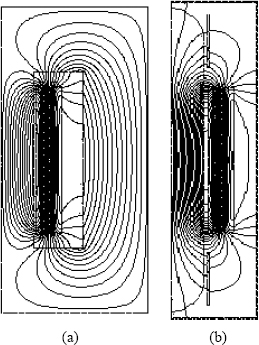
Figure 3.1 Leakage field in a transformer.

3.1    Reactance Calculation

3.1.1    Concentric primary and secondary windings

A transformer is a 3-D electromagnetic structure with the leakage field appreciably different in the core-window cross section (Figure 3.1 (a)) as compared to that in the cross section perpendicular to the window (Figure 3.1 (b)). Reactance (≅ impedance) values, however, can be estimated reasonably close to test values by considering only the window cross section. A high level of accuracy of 3-D calculations may not be necessary since the tolerance on reactance values is usually in the range of ± 7.5% or ± 10%.

For uniformly distributed ampere-turns along the LV and HV windings with equal heights, the leakage field is predominantly axial, except at the winding ends where there is fringing of the leakage flux which returns through a shorter path. A typical leakage field pattern shown in Figure 3.1 (a) can be replaced by a set of parallel flux lines of equal height as shown in Figure 3.2 (a). The equivalent height (H_eq) is obtained by dividing the winding height (H_w) by Rogowski factor K_R (< 1.0),

Figure 3.2 (a) Leakage field with equivalent height. (b) Magnetomotive force or flux density diagram.

$H_{eq}=\frac{H_w}{K_R}.$

(3.1)

The leakage magnetomotive (mmf) distribution across the cross section of the LV and HV windings is of the trapezoidal form as shown in Figure 3.2 (b). The mmf at any point depends on the ampere-turns enclosed by a flux contour at that point; it increases linearly with the enclosed ampere-turns from a value of zero at the inside diameter of the LV winding to the maximum value of one per-unit (the total ampere-turns of the LV or HV winding) at its outside diameter. In the gap (T_g) between the windings, since the flux contour at any point encloses the entire LV (or HV) ampere-turns, the mmf has a constant value. The mmf starts reducing linearly from the maximum value at the inside diameter of the HV winding until it becomes zero at its outside diameter. The core is assumed to have an infinite permeability value, thus, requiring no magnetizing mmf, and therefore the primary and secondary mmfs exactly balance each other. The flux density distribution is of the same form as that of the mmf distribution. Since the magnetic properties are assumed to be ideal, no mmf is expended in the return path of the flux through the core. Hence, for a closed contour of flux at a distance x from the inside diameter of the LV winding, it can be written that

$\left(\frac{B_x}{{\mu }_0}\right)H_{eq}={(NI)}_x$

(3.2)

or

$B_x=\frac{{\mu }_0{(NI)}_x}{H_{eq}}.$

(3.3)

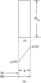
Figure 3.3 (a) Flux tube. (b) MMF diagram.

For deriving the formula for the leakage reactance, let us first obtain a general expression for the flux linkages of a flux tube having the radial depth R and the height H_eq. The ampere-turns enclosed by a flux contour at the inside diameter (ID) and outside diameter (OD) of this flux tube are a(NI) and b(NI), respectively as shown in Figure 3.3 (b), where NI are the rated ampere-turns. Such a general formulation is useful when a winding is split radially into a few sections separated by gaps. The r.m.s. value of the flux density at a distance x from the ID of this flux tube can now be inferred from Equation 3.3 as

$B_x=\frac{{\mu }_0}{H_{eq}}\left[\left(a+\frac{b-a}{R}x\right)NI\right].$

(3.4)

The flux linkages of an incremental flux tube of the width dx placed at x are

$d\psi =N_x{\varphi }_x=N_x{B}_{x}A,$

(3.5)

where A is the area of flux tube given by

$A=\pi (ID+2x)dx.$

(3.6)

Substituting Equations 3.4 and 3.6 in Equation 3.5, we obtain

$d\psi =\left\{\left(a+\frac{b-a}{R}x\right)N\right\}\left\{\frac{{\mu }_0}{H_{eq}}\left[\left(a+\frac{b-a}{R} x\right)NI\right]\right\}\left[\pi (ID+2x)dx\right].$

(3.7)

Hence, the total flux linkages of the flux tube are given by

$\psi =\underset{0}{\overset{R}{{\displaystyle \int }}}d\psi =\frac{{\mu }_0\pi N^{2}I}{H_{eq}}\underset{0}{\overset{R}{{\displaystyle \int }}}{\left(a+\frac{b-a}{R}x\right)}^2(ID+2x)dx.$

(3.8)

After integration and a few arithmetic operations, we obtain

$\psi =\frac{{\mu }_0\pi N^{2}I}{H_{eq}}\frac{R}{3}\left[(a^2+ab+b^2)ID+\frac{(a^2+ab+b^2)3R}{2}-\frac{2a^2+ab}{2}R\right].$

(3.9)

The last term in the square bracket can be neglected without introducing an appreciable error to arrive at a simple formula for the regular design use,

$\psi =\frac{{\mu }_0\pi N^{2}I}{H_{eq}}\frac{R}{3}(a^2+ab+b^2)\left[ID+\frac{3R}{2}\right].$

(3.10)

The term $\left[ID+\frac{3R}{2}\right]$ is approximately equal to the mean diameter (D_m) of the flux tube for large diameters of windings/gaps with comparatively lower values of their radial depths.

$\therefore \psi =\frac{{\mu }_0\pi N^{2}I}{H_{eq}}\frac{R}{3}(a^2+ab+b^2)D_m.$

(3.11)

Now, let

$ATD=\frac{R}{3}(a^2+ab+b^2)D_m$

(3.12)

which corresponds to the area of the mmf (ampere-turns) diagram. The leakage inductance of a transformer with n flux tubes can now be given as

$L=\frac{{\displaystyle \sum _{k=1}^n\psi }}{I}=\frac{{\mu }_0\pi N^2}{H_{eq}}{\displaystyle \sum }_{k=1}^{n}ATD,$

(3.13)

and the corresponding expression for the leakage reactance X is

$X=2\pi f=\frac{{\mu }_0\pi N^2}{H_{eq}}{\displaystyle \sum }_{k=1}^{n}ATD.$

(3.14)

The percentage leakage reactance, with the base impedance as Z_b, is given by

$\begin{array}{l}\%X=\frac{X}{Z_b}\times 100=\frac{IX}{V}\times 100=2\pi f\frac{{\mu }_0\pi I{N}^2}{H_{eq}V}{\displaystyle \sum }_{k=1}^{n}ATD\times 100\\ =2\pi f\frac{{\mu }_0\pi (NI)}{H_{eq}(V/N)}{\displaystyle \sum }_{k=1}^{n}ATD\times 100\end{array}$

(3.15)

where V is the rated voltage and the term (V/N) is volts/turn of the transformer. Substituting μ₀ = 4π × 10⁻⁷ and adjusting the constants so that the dimensions used in the formula are in units of centimeters (H_eq in cm and ${\displaystyle \sum ATD}$ in cm²), we obtain

$\%X=2.48\times {10}^{-5}f\frac{(AmpereTurns)}{H_{eq}(Volts/Turn)}{\displaystyle \sum }_{k=1}^{n}ATD.$

(3.16)

After having derived the general formula, we will now apply it for a simple case of a two winding transformer shown in Figure 3.2. The constants a and b have the values of 0 and 1 for the LV winding, 1 and 1 for the gap, and 1 and 0 for the HV winding, respectively. If D₁, D_g and D₂ are the mean diameters and T₁, T_g, and T₂ are the radial depths of the LV winding, the gap and the HV winding, respectively, using Equation 3.12 we have

${\displaystyle \sum ATD=\frac{1}{3}(T_1\times D_1)+(T_g\times D_g)+\frac{1}{3}(T_2\times D_2).}$

(3.17)

The value of H_eq is calculated by Equation 3.1, for which the Rogowski factor K_R is given by

$K_R=1-\frac{1-e^{-\pi H_w/(T_1+T_g+T_2)}}{\pi H_w/(T_1+T_g+T_2)}.$

(3.18)

For taking into account the effect of the core, a more accurate but complex expression for K_R can be used as given in [1]. For most cases, Equation 3.18 gives sufficiently accurate results.

For autotransformers, transformed ampere-turns should be used in Equation 3.16 (the difference between the turns corresponding to the phase voltages of the HV and LV windings multiplied by the HV winding current) and the calculated impedance is multiplied by the autofactor,

$K_A=1-\frac{V_{LV}}{V_{HV}}$

(3.19)

where V_LV and V_HV are the rated line voltages of the LV and HV windings respectively.

3.1.2    Sandwich windings

The reactance formula derived in the previous section can also be used for sandwich windings in core- or shell-type transformers with slight modifications. Figure 3.4 shows a configuration of such windings with two sections. The mean diameter of the windings is denoted by D_m. If there are N turns and S sections in the windings, then remembering the fact that the reactance is proportional to the square of turns, the reactance between the LV and HV windings corresponding to any one section (having N/S turns) is given by

$\%X_S=2.48\times {10}^{-5}f\frac{NI}{H_{eq}(V/N)}\frac{1}{S^2}{\displaystyle \sum }_{k=1}^{n}ATD$

(3.20)

where

${\displaystyle \sum }_{k=1}^{n}ATD=\frac{1}{3}\left(T_1\times D_m\right)+\left(T_g\times D_m\right)+\frac{1}{3}\left(T_2\times D_m\right)=D_m\left[T_g+\frac{T_1+T_2}{3}\right].$

(3.21)

If the sections are connected in series, the total reactance is S times that of a single section,

$\%X=2.48\times {10}^{-5}f\frac{NI}{H_{eq}(V/N)}\frac{1}{S}{\displaystyle \sum }_{k=1}^{n}ATD.$

(3.22)

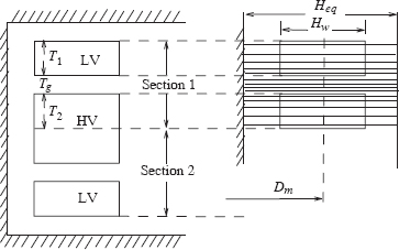
Figure 3.4 Sandwich winding.

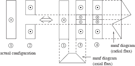
Figure 3.5 Unequal AT/m distribution.

Similarly, if the sections are connected in parallel, the formula can be derived by taking the number of turns as N and the current as I/S for a single section.

3.1.3    Concentric windings with nonuniform distribution of ampere turns

Since varying amounts of turns in the tap winding are excluded at different tap positions, the ampere-turns per unit height (AT/m) of the LV winding differ from those of the HV winding in the tap zone. This results in a higher amount of radial flux in such zones. When taps are in the main body of a winding (i.e., no separate tap winding), it is preferable to put taps symmetrically in the middle or at the ends of the winding to minimize the radial flux. If taps are provided only at one end, the arrangement causes an appreciable asymmetry and a higher radial component of the leakage flux resulting into increased eddy losses and axial short-circuit forces. For different values of AT/m along the height of the LV and HV windings, the reactance can be calculated by resolving the AT distribution as shown in Figure 3.5. The effect of the gap in winding 2 can be accounted for by replacing it with windings 3 and 4. Winding 3 has the same AT/m distribution as that of winding 1, and winding 4 has AT/m distribution such that the addition of the ampere-turns of windings 3 and 4 along their height gives the same ampere-turns as that of winding 2. The total reactance is the sum of the two reactances, the reactance between windings 1 and 3 calculated by Equation 3.16 and the reactance of winding 4 calculated by Equation 3.22 (for the sections connected in series).

Since Equation 3.22 always gives a finite positive value, a nonuniform AT distribution (unequal AT/m of the LV and HV windings) always results in a higher value of the reactance. An increased value of the reactance can be correlated with the fact that the effective height of the windings in Equation 3.16 is reduced if we take the average of the heights of windings 1 and 2. For example, if the tapped-out section in one of the windings is 5% of the total height at the tap position corresponding to the rated voltage, the average height is reduced by 2.5%, giving an increase in the reactance of 2.5% compared to the case of the uniform AT/m distribution.

3.2    Different Approaches for Reactance Calculation

The first approach is based on the fundamental definition of the inductance of a coil, i.e., flux linkages (ψ) per unit current (I),

$L=\frac{\psi }{I}=\frac{N\varphi }{I}$

(3.23)

and this approach has been used in Section 3.1 for finding the leakage inductance (Equations 3.13).

In another energy-based approach, it is calculated as

$L=\frac{2W_m}{I^2}$

(3.24)

where W_m is the stored magnetic energy by the current I flowing in a closed path. Now, we will see that the use of Equation 3.24 leads us to the same formula of the reactance as given by Equation 3.16.

The energy per unit volume in the magnetic field in the free space, with linear magnetic characteristics (H = B / μ₀), when the flux density is increased from 0 to B, is

$w=\underset{0}{\overset{B}{{\displaystyle \int }}}HdB=\underset{0}{\overset{B}{{\displaystyle \int }}}\frac{B}{{\mu }_0}dB=\frac{B^2}{2{\mu }_0}.$

(3.25)

A detailed discussion on the magnetic energy is available in Chapter 12. The differential energy dW_x for a cylindrical ring of height H_eq, thickness dx and diameter (ID + 2x) is

$d{W}_x=\frac{B_x^2}{2{\mu }_0}\times (volumeofcylindricalring)=\frac{B_x^2}{2{\mu }_0}\pi (ID+2x)H_{eq}dx.$

(3.26)

Now the value of B_x can be substituted from Equation 3.4 for the simple case of the flux tube with a = 0 and b = 1 (with reference to Figure 3.3),

$d{W}_x=\frac{{\mu }_0\pi {(NI)}^2{x}^2(ID+2x)dx}{2R^2{H}_{eq}}.$

(3.27)

For the winding configuration of Figure 3.2, the total energy stored in the LV winding (with the term R replaced by the radial depth T₁ of the LV winding) is

$W_1=\frac{{\mu }_0\pi {(NI)}^2}{2T_1^2{H}_{eq}}\underset{0}{\overset{T_1}{{\displaystyle \int }}}{x}^2(ID+2x)dx=\frac{{\mu }_0\pi {(NI)}^2}{2H_{eq}}\frac{1}{3}\left\{ID+\frac{3T_1}{2}\right\}{T}_1.$

(3.28)

As seen in Section 3.1.1, the term in the brackets can be approximated as the mean diameter (D₁) of the LV winding to obtain

$W_1=\frac{{\mu }_0\pi {(NI)}^2}{2H_{eq}}\frac{1}{3}{D}_1{T}_1.$

(3.29)

Similarly, the energy in the HV winding can be calculated as

$W_2=\frac{{\mu }_0\pi {(NI)}^2}{2H_{eq}}\frac{1}{3}{D}_2{T}_2.$

(3.30)

Since the flux density is constant in the gap between the windings, the energy in it can be directly calculated as

$W_g=\frac{B_g^2}{2{\mu }_0}\times (volumeofcylindricalgap)=\frac{1}{2{\mu }_0}{\left[\frac{{\mu }_0(NI)}{H_{eq}}\right]}^2\pi D_g{T}_g{H}_{eq}$

(3.31)

$\therefore W_g=\frac{{\mu }_0\pi {(NI)}^2}{2H_{eq}}{D}_g{T}_g.$

(3.32)

Substituting the values of the energies from Equations 3.29, 3.30 and 3.32 in Equation 3.24, we have

$L=\frac{2W_m}{I^2}=\frac{2(W_1+W_2+W_g)}{I^2}=\frac{{\mu }_0\pi N^2}{H_{eq}}\left[\frac{1}{3}(T_1{D}_1+T_2{D}_2)+T_g{D}_g\right].$

(3.33)

If the term in the brackets is substituted by ${\displaystyle \sum ATD}$ according to Equation 3.17, we see that the above expression derived from the energy viewpoint is the same as that in Equation 3.13 obtained from the flux linkages.

In yet another approach, when numerical methods like finite element method (FEM) are used, the field solution is usually obtained in terms of the magnetic vector potential, and the leakage inductance is given as

$L=\frac{1}{I^2}{\displaystyle \underset{vol}{\int }A\cdot Jdv,}$

(3.34)

where A is the magnetic vector potential and J is the current density vector. Equation 3.34 can be derived [2] from Equation 3.24,

$L=\frac{2W_m}{I^2}=\frac{1}{I^2}{\displaystyle \underset{vol}{\int }B\cdot Hdv=\frac{1}{I^2}}{\displaystyle \underset{vol}{\int }A\cdot Jdv.}$

(3.35)

The leakage reactance between two windings in a transformer can also be calculated as

$X_{12}=X_1+X_2-2M_{12}$

(3.36)

where X₁ and X₂ are the self reactances of the windings and M₁₂ is the mutual reactance between them. It is difficult to calculate the self and mutual reactances which depend on saturation effects. Also, since the values of (X₁ + X₂) and 2M₁₂ are nearly equal and are much higher than the leakage reactance X₁₂, a small error in the calculation of them results in a large error in the estimation of X₁₂. Hence, it is always easier to calculate the leakage reactance of a transformer directly instead of using the formulae in terms of the self and mutual reactances. Therefore, for finding the effective leakage reactance of a system of windings, the total power of the system is expressed in terms of the leakage impedances instead of the self and mutual impedances. Consider a system of windings 1, 2, …, n, with the leakage impedances Z_jk between the pairs of the windings j and k. For a negligible magnetizing current (as compared to the rated currents in the windings) the total power can be expressed as [3]

$P+jQ=-\frac{1}{2}{\displaystyle \sum }_{k=1}^n{\displaystyle \sum }_{j=1}^n{\widehat{Z}}_{jk}{\widehat{I}}_j{\widehat{I}}_k^{*}$

(3.37)

where ${\widehat{I}}_k^{*}$ is the complex conjugate of ${\widehat{I}}_k$. Winding resistances can be neglected in comparison with much larger leakage reactances. When the current vectors of the windings are parallel (in phase or phase-opposition), the expression for Q (which is given by the imaginary part of the previous equation) becomes

$Q=\text{ Im }\left[-\frac{1}{2}{\displaystyle \sum }_{k=1}^n{\displaystyle \sum }_{j=1}^n{\widehat{Z}}_{jk}{\widehat{I}}_j{\widehat{I}}_k^{*}\right]=-\frac{1}{2}{\displaystyle \sum }_{k=1}^n{\displaystyle \sum }_{j=1}^n{X}_{jk}{I}_j{I}_k.$

(3.38)

Equation 3.38 gives the total reactive volt-amperes consumed by all the leakage reactances of the system of the windings. The effective or equivalent leakage reactance of the system of n windings, referred to the source (primary) winding carrying the current I_p, is given by

$X_{eff}=\frac{Q}{I_p^2}\text{in}\text{Ω}\text{.}$

(3.39)

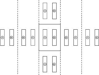
Figure 3.6 Method of images.

If the currents and X_jk are expressed in per-unit in Equation 3.38, the value of Q (calculated when the rated current flows in the primary winding) gives directly the per-unit reactance of the transformer consisting of n windings. The use of this reactive KVA approach is illustrated in Sections 3.6 and 3.7.

3.3    Analytical Methods

The classical method described in Section 3.1 has certain limitations. The effect of the core is neglected and it is tedious to take into account axial gaps in windings and asymmetries in distributions of ampere-turns. Some of the more commonly used analytical methods, which overcome these difficulties, are now described. The leakage reactance calculation by more accurate numerical methods (e.g., FEM) is described in Section 3.4.

3.3.1    Method of images

When computers were not available, many attempts were made to devise accurate methods of calculating axial and radial components of the leakage field, and subsequently the leakage reactance. A popular approach was to use simple Biot-Savart’s law with the effect of the iron core taken into account by the method of images. The method basically works in the Cartesian (x-y) coordinate system in which windings are represented by straight coils (assumed to be of infinite dimensions along the z-axis perpendicular to the plane of the paper) placed at appropriate distances from a plane surface bounding a semi-infinite mass of infinite permeability. The effect of the iron core is represented by the images of the coils as far behind the surface as they are in the front. Parallel planes have to be added as shown in Figure 3.6 to obtain accurate results, which leads to an arrangement of infinite images in all the four directions [4]. All these coils should give the same value of the leakage field at any point as that with the original geometry of the two windings enclosed by the iron boundary. New planes (mirrors) can be added, one at a time, until the difference between the successive solutions is negligible; usually the first three or four images are sufficient. Biot-Savart’s law is then applied to this arrangement of the current distributions, which is devoid of the magnetic mass (iron), to find the value of the leakage field at any point.

3.3.2    Roth’s method

A method based on double Fourier series, originally proposed by Roth, was extended in [5] to calculate the leakage reactance for an irregular arrangement of windings. The advantage of this method is that it is applicable to uniform as well as nonuniform distributions of ampere-turns of windings. The arrangement of windings in the core window can be entirely arbitrary but it should be divisible into rectangular blocks, each block having a uniform current density distribution within itself.

In this method, the core window is considered as π radians wide and π radians long, regardless of its absolute dimensions. The ampere-turn density distribution as well as the flux distribution is conceived to be consisting of components which vary harmonically along both the x and y axes. The method uses a principle similar to that of the method of images; for every harmonic the maximum value occurs at fictitious planes about which mirroring is done to simulate the effect of the iron boundary. Reactive volt-amperes (I² X) are calculated in terms of these current harmonics for a depth of unit dimension in the z direction. The total volt-amperes are obtained by multiplying the calculated values by corresponding mean perimeters. The per-unit value of the leakage reactance is calculated by dividing I² X by the base volt-amperes. For a reasonable accuracy, the number of space harmonics in the double Fourier series should be at least equal to 20 when the ampere-turns are symmetrically distributed in the LV and HV windings [6]. The accuracy is better with a higher number of space harmonics. Figure 3.7 shows plots of the radial flux density along the height of a transformer winding. As the number of the space harmonics is increased, the variation of the flux density becomes smooth indicating a better accuracy.

3.3.3    Rabin’s method

If the effect of curvatures of the windings needs to be taken into account in Roth’s formulation, the method becomes complicated, and in that case Rabin’s method is more suitable [4, 7]. It solves the following Poisson’s equation in cylindrical coordinates,

${\nabla }^{2}A=-\mu J$

(3.40)

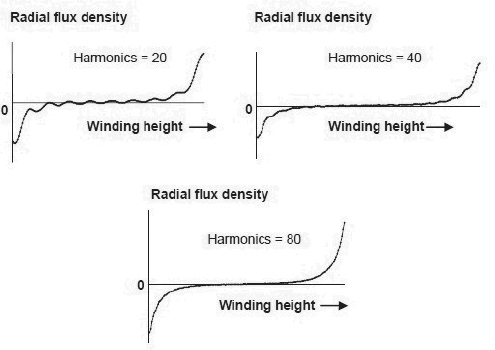
Figure 3.7 The effect of the number of space harmonics on the accuracy.

where A is the magnetic vector potential and J is the current density having only the angular component. Therefore, in cylindrical coordinates the equation becomes

$\frac{{\partial }^2{A}_{\theta }}{\partial r^2}+\frac{1}{r}\frac{\partial A_{\theta }}{\partial r}-\frac{A_{\theta }}{r^2}+\frac{{\partial }^2{A}_{\theta }}{\partial z^2}=-\mu J_{\theta }.$

(3.41)

In this method, the current density is assumed to depend only on the axial position and hence can be represented by a single Fourier series with coefficients which are Bessel and Struve functions. For a reasonable accuracy, the number of space harmonics should be about 70 [6].

3.4    Numerical Method for Reactance Calculation

The finite element method (FEM) is the most commonly used numerical method for the reactance calculation of nonstandard configurations of windings and asymmetrical/nonuniform distributions of ampere-turns, which cannot be easily and accurately handled by the classical method given in Section 3.1. The FEM analysis can be more accurate than the analytical methods described in Section 3.3. User-friendly commercial FEM software packages are now available. A 2-D FEM analysis can be integrated into routine design calculations. The main advantage of FEM is that any complex geometry can be analyzed since its formulation depends only on the class of problem and is independent of geometrical details. It can also take into account material discontinuities easily. The theory of the FEM technique and its applications to transformers are elaborated in Chapter 12. Here, the technique is briefly illustrated when applied to calculate the leakage reactance of a transformer.

The problem geometry is divided into small elements [8, 9]. Within each element, the flux density is assumed constant so that the magnetic vector potential varies linearly within each element (a first order approximation); in Cartesian coordinates the potential can be approximated as

$A=a+bx+cy.$

(3.42)

For a better accuracy, the potential can be assumed to vary as a polynomial of a degree higher than one. The elements are generally of triangular or tetrahedral shape. The windings are modeled as rectangular blocks; if the distribution of ampere-turns is not uniform, they are divided into suitable sections so that the current density in each section is uniform. A typical configuration of the LV and HV windings in a transformer is shown in Figure 3.8. The main steps involved in the analysis are now outlined.

1. Creation of geometry: The geometry shown in Figure 3.8 is simple. In case of complex 2-D or 3-D geometries, many commercial FEM programs allow the import of figures drawn in drafting packages, which makes it easier and less time consuming to create geometries. The problem domain has to be always bounded by a boundary (e.g., abcda in Figure 3.8). 2-D problems can be solved either in Cartesian or cylindrical coordinates. Since transformers are 3-D structures, both the systems lead to approximations and corresponding errors.

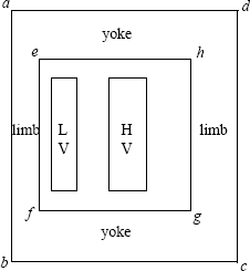
Figure 3.8 Geometry for FEM analysis.

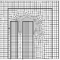
Figure 3.9 FEM mesh.

However, they give reasonably accurate results when used to calculate the leakage reactance in two dimensions. In the cylindrical coordinate system, line ab represents the axis (center line) of the core and the horizontal distance between the lines ab and ef equals half the core diameter.

2. Meshing: This step involves division of the geometry into small elements. For most accurate results, sizes of the elements should be as small as possible if the first order approximation is used. Thus, logically the element (mesh) size should be small only in the regions where there are significant variations in values of the flux density. Such an intelligent meshing reduces the number of elements and the computation time. An inexperienced person may not always know the regions where the solution changes significantly; hence a solution with a coarse mesh can be obtained first, and then the mesh can be refined in the regions where the solution is changing rapidly. Ideally, one has to go on refining the mesh until there is no appreciable change in the value of the solution (the flux density in this case) at any point in the geometry. For the problem domain in Figure 3.8, the radial component of the flux density changes considerably at the ends of the windings, necessitating the use of a finer mesh in these regions as shown in Figure 3.9.

3. Material properties: The relative permeability (μ_r) of the core is specified as a few tens of thousands. It really does not matter whether we define it as 10000 or 50000 because almost all the energy is stored in the nonmagnetic regions (μ_r =1) outside the core. While estimating the leakage reactance, the ampere-turns of the LV and HV windings are assumed to be exactly equal and opposite (the no-load current is neglected), and hence according to Ampere’s circuital law there is not a single flux contour in the core enclosing both the windings (see Chapter 12 for a detailed discussion). Other parts, including windings, are defined with μ_r of 1. It should be remembered that copper/aluminum is a non-magnetic material. Here, the conductivity of the winding material is not defined since the effect of eddy currents in winding conductors on the leakage field is usually neglected in the reactance calculation; the problem is solved as a magnetostatic problem. Individual conductors/turns may have to be modeled for the estimation of circulating currents in parallel conductors, which is a subject of discussion in Chapter 4.

4. Source definition: In this step, the density of ampere-turns for each winding or section is defined (i.e., the ampere-turns divided by the cross-sectional area).

5. Boundary conditions: There are two types of boundary conditions, viz., Dirichlet and Neumann. When a potential value is prescribed on a boundary, it is called the Dirichlet boundary condition. In the present case, the Dirichlet condition is defined for the boundary abcda (flux lines are parallel to this boundary) with the value of the magnetic vector potential taken as zero for convenience. It should be noted that a contour passing through equal values of the magnetic vector potential is a flux line. A boundary, on which the normal derivative of a potential is specified, is said to have the Neumann condition. Flux lines cross perpendicularly at these boundaries. A boundary on which the Dirichlet condition is not defined, the Neumann condition gets automatically specified in the FEM formulation. If the core is not modeled, no magnetic vector potential should be defined on the boundary efgh (iron-air boundary). The flux lines then impinge perpendicularly on this boundary, which is in line with the valid assumption that the core is infinitely permeable for the problem under consideration. When the core is not modeled, one reference potential may have to be defined; zero potential can be specified at a point in the gap between the two windings along their center line in the present case.

6. Solution: Formations of element level coefficient matrices, the assembly of the global coefficient matrix and the imposition of boundary conditions are done in this step; commercial FEM programs do these things internally. For a detailed explanation of the FEM procedure, refer to Chapter 12.

7. Post-processing: A leakage field plot (Figure 3.1a) can be obtained and studied in this step. The total stored energy is calculated as

$W_m=\frac{1}{2}{\displaystyle \underset{vol}{\int }A\cdot Jdv.}$

(3.43)

If the problem is solved in Cartesian coordinates, the energy per unit length in the z direction is obtained. In order to obtain the total energy, the magnitude of the energy for each section of the geometry is multiplied by the corresponding mean turn length (i.e., π × mean diameter). Finally, the leakage inductance can be calculated using Equation 3.24.

Example 3.1

Relevant dimensions (in mm) of a 31.5 MVA, 132/33 kV, 50 Hz, Yd1 transformer are indicated in Figure 3.10. The value of volts/turn is 76.21. The transformer is having 0% to +10% taps on the HV winding. It is having a linear-type on-load tap changer; 10% tapping turns are placed symmetrically in the middle of the HV winding for giving the total voltage variation of 10%. It is required to calculate the leakage reactance of the transformer at the nominal tap position (corresponding to the HV voltage of 132 kV) by the classical method and the FEM analysis.

Solution:

We will calculate the leakage reactance by the method given in Section 3.1.3 as well as by the FEM analysis.

1. Classical method

At the nominal tap position, TAP winding has zero ampere-turns since all its turns are cut out of the circuit. This results into an unequal AT/m distribution between the LV and HV windings along their heights.

$\text{HV current}=\frac{31.5\times {10}^6}{\sqrt{3}\times 132\times {10}^3}=137.78\text{A}.$

$\text{HV turns}=\frac{132\times {10}^3/\sqrt{3}}{76.21}=1000\text{and}\text{LV}\text{turns}=\frac{33\times {10}^3}{76.21}=433.$

The HV winding is replaced by a winding (HV1) with uniformly distributed ampere-turns (1000 turns are distributed uniformly along the height of 1260 mm) and a second winding (HV2) having the distribution of ampere-turns such that the superimposition of the ampere-turns of both the windings gives that of the original HV winding.

We will first calculate the reactance between the LV and HV1 windings by using the procedure given in Section 3.1.

T₁ = 7.0 cm, T₂ = 5.0 cm, T₃ = 10.0 cm, H_w = 126.0 cm.

Equations 3.18 and 3.1 give

K_R = 0.944 and H_eq = H_w/K_R = 126/0.944 = 133.4 cm.

The term ${\displaystyle \sum ATD}$ is calculated as per Equation 3.17,

${\displaystyle \sum ATD=\frac{1}{3}\times 7.0\times 67.6+5.0\times 79.6+\frac{1}{3}\times 10.0\times 94.6=871.1{\text{cm}}^2.}$

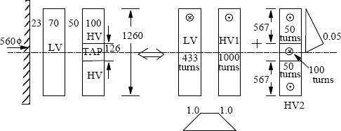
Figure 3.10 Details of the transformer in Example 3.1.

The leakage reactance can be calculated from Equation 3.16 as

$X_{{\text{LV}}_{-}\text{HV}1}=2.48\times {10}^{-5}\times 50\times \frac{(137.78\times 1000)}{133.4\times 76.21}\times 871.1=14.64\%.$

The winding HV2 is made up of two sections. The AT diagram for the top section is shown in Figure 3.10. The section has two windings, each having ampere-turns of 0.05 per-unit [= (50×137.78)/(1000×137.78)]. For this section,

T₁ = 56.7 cm, T_g = 0.0 cm, T₂ = 6.3 cm, H_w = 10.0 cm.

It is to be noted here that the winding height for the calculation is the dimension in the radial direction, which is equal to 10.0 cm. Equations 3.18 and 3.1 give

K_R = 0.213 and H_eq = H_w/K_R = 10/0.213 = 47.0 cm.

The term ATD is calculated for each part using Equation 3.12, the corresponding values of a and b, and the mean diameter of the HV winding,

${\displaystyle \sum ATD=\frac{56.7}{3}\times {0.05}^2\times 94.6+0.0\times {0.05}^2\times 94.6+\frac{6.3}{3}\times {0.05}^2\times 94.6=\mathrm{5.0.}}$

The leakage reactance of the section can be calculated from Equation 3.16 as

$X_S=2.48\times {10}^{-5}\times 50\times \frac{(137.78\times 1000)}{470\times 76.21}\times 5.0=0.24\%.$

The HV2 winding comprises of two such sections connected in series. Hence, the total reactance contributed by the HV2 winding is two times the reactance of a single section as explained in Section 3.1.2.

∴ X_HV2 = 2 × 0.24 = 0.48%.

Therefore, the total reactance is

X = X_{LV_HV1} + X_HV2 = 14.64 + 0.48 = 15.12 %.

2. FEM analysis

The analysis is done as per the steps outlined in Section 3.4. The winding to yoke distance is 130 mm for this transformer. The stored energies in the different parts of the geometry as given by the FEM analysis are:

LV winding:	438 J
HV winding:	773 J
HV winding - center gap:	87 J
Remaining portion:	1205 J

The energy stored in the core is negligible; the total energy obtained is 2503 J. Using Equation 3.24, the leakage inductance is calculated as

$L=\frac{2\times 2503}{{(137.78)}^2}=0.264\text{H}\text{.}$

The value of the base impedance is

$Z_b=\frac{{\text{kV}}^{\text{2}}}{\text{MVA}}=\frac{{132}^2}{31.5}=553.1\text{Ω}.$

$\therefore X=\frac{2\pi \times 50\times L}{Z_b}\times 100=\frac{2\pi \times 50\times 0.264}{553.1}\times 100=15.0\%.$

Thus, the values of the leakage reactance given by the classical method and the FEM analysis are in close agreement.

Example 3.2

Calculate the leakage reactance of a transformer having 10800 ampere-turns in each of the LV and HV windings. The rated voltage and current of the LV winding are 415 V and 300 A, respectively. The two windings are sandwiched into 4 sections as shown in Figure 3.11. Relevant dimensions (in mm) are given in the figure. The value of volts/turn is 11.527. The mean diameter of the windings is 470 mm.

Solution:

The leakage reactance will be calculated by the method given in Section 3.1.2 and the FEM analysis.

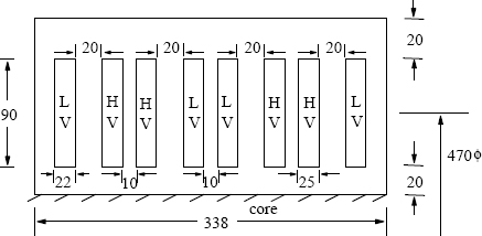
Figure 3.11 Details of the transformer in Example 3.2.

1. Classical method

The whole configuration consists of four sections, each having 1/4 part of both the LV and HV windings. For each section,

T₁ = 2.2 cm, T_g = 2.0 cm, T₂ = 2.5 cm, H_w = 9.0 cm.

Equations 3.18 and 3.1 give

K_R = 0.767 and H_eq = H_w/K_R = 9/0.767 = 11.7 cm.

The term ${\displaystyle \sum ATD}$ is (Equation 3.17)

${\displaystyle \sum ATD=\frac{1}{3}\times 2.2\times 47.0+2.0\times 47.0+\frac{1}{3}\times 2.5\times 47.0=\mathrm{167.6.}}$

The leakage reactance between the LV and HV windings can be calculated from Equation 3.22 with 4 sections,

$\%X=2.48\times {10}^{-5}\times 50\times \frac{10800}{11.7\times 11.527}\times \frac{1}{4}\times 167.6=4.16\%.$

2. FEM analysis

The geometry as given in Figure 3.11 is modeled and an analysis is carried out according to the steps outlined in Section 3.4. The stored energy in the different parts of the geometry is:

LV (all 4 parts):	1.44 J
HV (all 4 parts):	1.66 J
Remaining portion:	5.26 J

The total energy is 8.36 J. Using Equation 3.24, the leakage inductance is calculated as

$L=\frac{2\times 8.36}{{(300)}^2}=0.000186\text{H}\text{.}$

The base impedance value is

$Z_b=\frac{\text{Rated}\text{voltage}}{\text{Rated}\text{current}}=\frac{415}{300}=1.38\text{Ω}.$

$\therefore X=\frac{2\pi \times 50\times L}{Z_b}\times 100=\frac{2\pi \times 50\times 0.000186}{1.38}\times 100=4.23\%.$

3.5    Impedance Characteristics of Three-Winding Transformers

A three-winding (three-circuit) transformer is required when actual loads or auxiliary loads (reactive power compensating devices such as shunt reactors or condensers) are required to be supplied at a voltage different from the primary and secondary voltages. An unloaded tertiary winding is commonly used for the stabilizing purpose as discussed in Section 3.8.

The characteristics and issues related to the leakage field (efficiency, regulation, parallel operation, and short-circuit currents) of a multi-circuit transformer cannot be analyzed in the same way as that for a two-winding transformer. The leakage reactance characteristics of a three-winding transformer can be represented by an equivalent circuit, for doing which it is assumed that each winding has its own individual leakage reactance. When the magnetizing current is neglected (which is justified in the calculations related to leakage fields) and if all the quantities are expressed in the per-unit or percentage notation, the magnetically interlinked circuits of the three-winding transformer can be represented by electrically interlinked circuits as shown in Figure 3.12. The equivalent circuit can be either a star or mesh network. The star equivalent circuit is more commonly used and is discussed here.

The percentage leakage reactances between pairs of windings can be expressed in terms of their individual percentage leakage reactances (all expressed on a common base of volt-amperes) as

$X_{12}=X_1+X_2$

(3.44)

$X_{23}=X_2+X_3$

(3.45)

$X_{31}=X_1+X_3.$

(3.46)

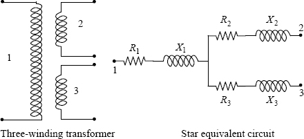
Figure 3.12 Representation of a three-winding transformer.

It follows from the above three equations that the individual reactances in the star equivalent circuit are given by

$X_1=\frac{1}{2}\left[X_{12}+X_{13}-X_{23}\right]$

(3.47)

$X_2=\frac{1}{2}\left[X_{12}+X_{23}-X_{13}\right]$

(3.48)

$X_3=\frac{1}{2}\left[X_{13}+X_{23}-X_{12}\right].$

(3.49)

A rigorous derivation of the above three equations and the evolution of the star equivalent circuit is given in [10].

Similarly, the percentage resistances can be derived as

$R_1=\frac{1}{2}\left[R_{12}+R_{13}-R_{23}\right]$

(3.50)

$R_2=\frac{1}{2}\left[R_{12}+R_{23}-R_{13}\right]$

(3.51)

$R_3=\frac{1}{2}\left[R_{13}+R_{23}-R_{12}\right].$

(3.52)

Note that these percentage resistances represent the total load loss (the addition of the DC-resistance I² R loss in windings, the eddy loss in windings and the stray loss in structural parts).

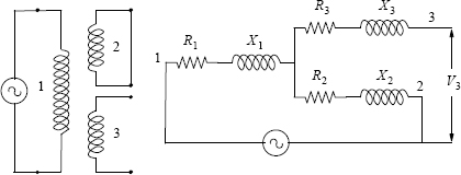
Figure 3.13 Mutual effect in star equivalent network.

The leakage reactances in the star equivalent network are basically the mutual load reactances between different circuits. For example, the reactance X₁ in Figure 3.12 is the common or mutual reactance to the loads in circuits 2 and 3. A current flowing from circuit 1 to either circuit 2 or 3 produces voltage drops across R₁ and X₁, and hence affects the voltages in circuits 2 and 3. When a voltage is applied to winding 1 with winding 2 short-circuited as shown in Figure 3.13, the voltage across the open-circuited winding 3 is equal to the voltage drop across the leakage impedance, Z₂, of circuit 2.

The individual leakage reactance of a winding can be negative. The total leakage reactance between a pair of windings cannot be negative but the mutual effect between two circuits may be negative when a load current flows [11]. Negative impedances are virtual values, and they reproduce faithfully the terminal characteristics of transformers. The three windings are interlinked, and hence a load current flowing in a winding affects the voltages in the other two windings, sometimes in a surprising way. For example, a lagging load on a winding may increase the voltage magnitude of another winding due to the presence of a negative value of a leakage reactance (capacitive reactance) in the equivalent circuit.

Similarly, a negative resistance may appear in the star equivalent network of an autotransformer with a tertiary winding or of a high efficiency transformer whose stray loss is much higher as compared to the ohmic losses in its windings (e.g., when a lower value of the current density is used for the windings).

In Chapter 1, we have seen how the regulation of a two-winding transformer is calculated. The calculation of the voltage regulation of a three-winding transformer is explained with the help of the following example.

Example 3.3

Find the voltage drop between the terminals of a three-winding transformer, when the load on the IV winding is 70 MVA at 0.8 lagging power factor, and the load on the LV winding is 30 MVA at 0.6 lagging power factor. The transformer data is:

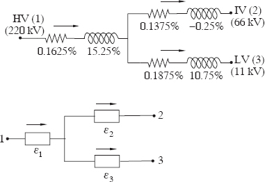
Figure 3.14 Star equivalent circuit and regulation (Example 3.3).

Rating: 100/100/30 MVA, 220/66/11 kV

Results of short circuit tests referred to 100 MVA base:

$\begin{array}{lll}\text{HV-IV}\hfill & :R_{1-2}=0.30\%,\hfill & X_{1-2}=15.0\%\hfill \\ \text{HV-LV}\hfill & :R_{1-3}=0.35\%,\hfill & X_{1-3}=26.0\%\hfill \\ \text{IV-LV}\hfill & :R_{2-3}=0.325\%,\hfill & X_{2-3}=10.5\%\hfill \end{array}$

Solution:

The star equivalent circuit derived using Equations 3.47 to 3.52 is shown in Figure 3.14. It is to be noted that although the HV, IV and LV windings are rated for different MVA values, for finding the equivalent circuit, we have to work on a common MVA base (in this case it is 100 MVA).

The IV winding is loaded to 70 MVA; let the constant K₂ denote the ratio of the actual load to the base MVA,

K₂ = 70/100 = 0.7.

Similarly, for the LV winding which is loaded to 30 MVA,

K₃ = 30/100 = 0.3.

The voltage drops for circuits 2 and 3 are calculated using Equation 1.65,

$\begin{array}{l}{\epsilon }_2=K_2(R_2\text{cos}{\theta }_2+X_2\text{sin}{\theta }_2)=0.7(0.1375\times 0.8+(-0.25)\times 0.6)=-0.03\%\\ {\epsilon }_3=K_3(R_3\text{ cos}{\theta }_3+X_3\text{ sin}{\theta }_3)=0.3(0.1875\times 0.6+10.75\times 0.8)=2.61\%.\end{array}$

The effective power factor (cosθ₁) and the effective load taken as a fraction (K₁) of the base MVA for the primary (220 kV) circuit are determined by solving the following two equations:

$K_1\text{cos}{\theta }_1=K_2\text{cos}{\theta }_2+K_3\text{ cos}{\theta }_3=0.7\times 0.8+0.3\times 0.6=0.74$

(3.53)

$K_1\text{sin}{\theta }_1=K_2\text{sin}{\theta }_2+K_3\text{sin}{\theta }_3=0.7\times 0.6+0.3\times 0.8=0.66$

(3.54)

Solving these two equations we obtain

K₁ = 0.99, cosθ₁ = 0.75, sinθ₁ = 0.67.

Therefore, the primary circuit voltage drop (regulation) is

ε₁ = K₁ (R₁ cosθ₁ + X₁ sinθ₁) = 0.99(0.1625 × 0.75 + 15.25 × 0.67)= 10.23%.

Now, the voltage drops between the terminals can be calculated as

$\begin{array}{l}{\epsilon }_{1-2}={\epsilon }_1+{\epsilon }_2=10.23+(-0.03)=10.2\%\\ {\epsilon }_{1-3}={\epsilon }_1+{\epsilon }_3=10.23+2.61=12.84\%\\ {\epsilon }_{2-3}=-{\epsilon }_2+{\epsilon }_3=0.03+2.61=2.64\%.\end{array}$

While calculating ε₂₋₃, a minus sign is used for ε₂ as the drop in the voltage is in the direction opposite to the direction of the corresponding current flow.

When there are more than three windings, transformers cannot be in general represented by a pure star or mesh equivalent circuit. The equivalent circuit should have n (n −1) / 2 independent impedance links, where n is the number of windings. A four-winding transformer has six independent links with four terminal points. The procedure for determining the values of impedances in the equivalent circuit of a transformer having four or more windings is given in [1, 12, 13].

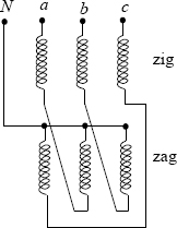
Figure 3.15 A zigzag connection.

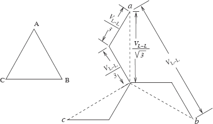
Figure 3.16 Vector diagram of a delta-zigzag transformer.

3.6    Reactance Calculation for Zigzag Transformers

A zigzag connection, in which the windings on different limbs are cross-connected, is shown in Figure 3.15. It is termed zigzag or interconnected star winding because the zig winding of one phase is connected in series with the zag winding of one of the other two phases. The vector diagram of a delta-zigzag transformer is shown in Figure 3.16. The interconnection of the windings of different phases introduces a phase shift of 30° (or 150°) between the zig (or zag) winding and the corresponding line-to-neutral voltage ($V_{L-N}=V_{L-L}/\sqrt{3}$). The zig and zag windings have 15.47% more turns than conventional windings to obtain the same magnitude of phase/line voltages. Hence, zigzag transformers are costlier than conventional transformers, but its use is essential in some cases. Their main characteristics and advantages are as follows:

•  They can be used as an earthing transformer in a delta-connected system or an ungrounded star-connected system, wherein a neutral point is not available for the earthing (grounding) purpose. Consider a zigzag transformer connected to a delta-connected source as shown in Figure 3.17. For a single line-to-ground fault, a zero-sequence current flows in the ground circuit allowing a protection system to act. The voltages of the two healthy line terminals are maintained at their respective line-to-neutral voltage levels. In the absence of the grounded neutral connection, the voltages of the healthy phases increase to the line-to-line voltage level, stressing insulation systems of the connected equipment. Thus, the zigzag earthing transformers not only aid the protection system but also reduce the voltage stresses under asymmetrical fault conditions.

Figure 3.17 A zigzag earthing transformer.

•  Zigzag transformers offer a specific advantage when used in applications consisting of power electronic converters. The DC magnetization due to asymmetry in firing angles is cancelled in each limb due to opposite directions of the DC currents flowing in its zig and zag windings. Similarly, the DC magnetization inherent in a three-pulse mid point rectifier connection is eliminated if the secondary winding is of zigzag type [14].

•  Earthing transformers offer a low impedance path to zero-sequence currents under asymmetrical fault conditions because the only magnetic flux produced by the currents is the leakage flux; the magnetizing flux in each limb is zero due to the equal and opposite currents flowing in its zig and zag windings as shown in Figure 3.17. Owing to a very low impedance of the earthing transformer, it may be necessary to limit currents under fault conditions by connecting a resistor between the neutral and the earth. Under normal operating conditions, only a small exciting current flows in the windings of the earthing transformer.

•  Third harmonic voltage components present in the zig and zag windings are cancelled in the lines.

The reactance of a transformer consisting of zigzag and star (or delta) windings can be calculated from reactive volt-amperes. Consider the star-zigzag transformer shown in Figure 3.18. The currents I_a, I_b and I_c are assumed to flow from the line terminals to the neutral for convenience. The corresponding vector diagram is also shown in the figure.

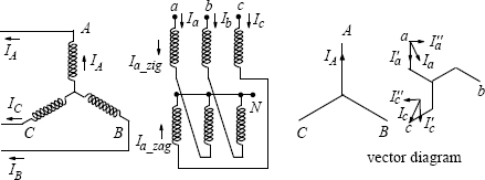
Figure 3.18 Reactance calculation of a transformer having a zigzag winding.

All the currents are resolved into two mutually perpendicular sets of components. Since the vector sum of all ampere-turns is zero on each limb, the sum of all the components indicated by prime is zero and the sum of all the components indicated by double prime is also zero. The current of the phase A of the star connected winding (I_A) is taken as the reference vector, and all the other currents are resolved in the directions along and perpendicular to this vector. Since I_A is the reference vector, $I_A^{\prime }$ and $I_A^{″}$ have the values 1 p.u. and 0 p.u., respectively, in per-unit notations. I_{a_zig} is in phase with I_a, whereas I_{a_zag} is in phase with I_c. The zig and zag windings have 0.577 p.u. ampere-turns (1.1547 × 0.5). Also, the currents I_a and I_c are at an angle of 30° with respect to the reference vector. The direction of I_c (I_{a_zag}) has been reversed in the vector diagram so that at any instant the corresponding ampere-turns of the zag winding oppose that of the star winding. Thus, we can write

$I_A^{\prime }=1,$

(3.55)

$I_A^{″}=0,$

(3.56)

$(I_{a_{-}zig}{)}^{\prime }=(I_{a_{-}zag}{)}^{\prime }=-0.577\text{cos }{30}^o=-0.5,\text{and}$

(3.57)

$(I_{a_{-}zig}{)}^{″}=-(I_{a_{-}zag}{)}^{″}=0.577\text{sin}30°=\mathrm{0.289.}$

(3.58)

Equations 3.55 to 3.58 satisfy the following two equations as required by the condition that the vector sum of all the ampere-turns on the limb of the phase A is zero:

$I_A^{\prime }+(I_{a_{-}zig}{)}^{\prime }+(I_{a_{-}zag}{)}^{\prime }=0\text{and}$

(3.59)

${I^{″}}_A+(I_{a_{-}zig}{)}^{″}+(I_{a_{-}zag}{)}^{″}=0.$

(3.60)

The vectors of the currents in the windings resolved into two mutually perpendicular sets can be used in conjunction with Equation 3.37 to calculate reactive volt-amperes (Q). The resistances of the windings are neglected since they are much lower than the reactances. The expressions of Q for the two sets are added algebraically,

$Q=-\frac{1}{2}{\displaystyle \sum }_{k=1}^n{\displaystyle \sum }_{j=1}^n{X}_{jk}(I_j{)}^{\prime }(I_k{)}^{\prime }-\frac{1}{2}{\displaystyle \sum }_{k=1}^n{\displaystyle \sum }_{j=1}^n{X}_{jk}(I_j{)}^{″}(I_k{)}^{″}.$

(3.61)

The expression of Q for the phase A having three windings, star, zig, and zag, denoted by numbers 1, 2, and 3, respectively, is

$\begin{array}{l}Q=-\frac{1}{2}\left\{2X_{12}{I^{\prime }}_1{I^{\prime }}_2+2X_{13}{I^{\prime }}_1{I^{\prime }}_3+2X_{23}{I^{\prime }}_2{I^{\prime }}_3\right\}\\ -\frac{1}{2}\left\{2X_{12}{I^{″}}_1{I^{″}}_2+2X_{13}{I^{″}}_1{I^{″}}_3+2X_{23}{I^{″}}_2{I^{″}}_3\right\}\end{array}$

(3.62)

where X₁₂, X₁₃, and X₂₃ are the per-unit leakage reactances between the corresponding windings. Substituting from Equations 3.55 to 3.58, and remembering that I₁ = I_A, I₂ = I_{a_zig} and I₃ = I_{a_zag},

$\begin{array}{l}Q=-\left\{X_{12}\times 1\times (-0.5)+X_{13}\times 1\times (-0.5)+X_{23}\times (-0.5)\times (-0.5)\right\}\\ -\left\{0+0+X_{23}\times 0.289\times (-0.289)\right\}\end{array}$

Since the currents and reactances are expressed in the per-unit notation, the value of Q directly gives the per-unit reactance of the star/zigzag transformer.

$\therefore Q=X_{{\text{star}}_{-}\text{zigzag}}=\frac{1}{2}\left[X_{12}+X_{13}\right]-\frac{1}{6}{X}_{23}.$

(3.63)

Thus, the leakage reactance of a transformer having star- (or delta-) and zigzag-connected windings can be computed easily, once the leakage reactances between the pairs of the windings are calculated using a common VA base.

Example 3.4

Find the leakage reactance of a 31.5 MVA, 132/11 kV, 50 Hz, star/zigzag transformer whose various relevant dimensions (in mm) are indicated in Figure 3.19. The value of volts/turn is 76.39.

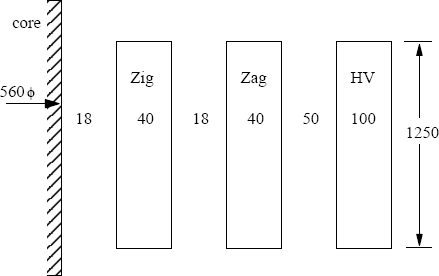
Figure 3.19 Dimensions of the star/zigzag transformer in Example 3.4.

Solution:

Let us first calculate the leakage reactances between the pairs of the windings, zig and zag, zig and HV, and zag and HV by the procedure given in Section 3.1.1 for concentric windings.

Reactance between the zig and zag windings:

$\begin{array}{cccc}{T}_1=4.0\text{cm,}& T_g=1.8\text{cm,}& T_2=4.0\text{cm,}& H_w=125.0\text{cm}\end{array}$

Equations 3.18 and 3.1 give K_R = 0.975 and H_eq = 125/0.975 = 128.2 cm. Equation 3.17 gives

${\displaystyle \sum ATD=\frac{1}{3}\times 4.0\times 63.6+1.8\times 69.4+\frac{1}{3}\times 4.0\times 75.2=310{\text{cm}}^2.}$

The reactance needs to be calculated using a common MVA base. The base volt-amperes are taken as 31.5 MVA. The corresponding current and turns of the HV winding should be used in the reactance formula.

$\text{HV current}=\frac{31.5\times {10}^6}{\sqrt{3}\times 132\times {10}^3}=137.78\text{A}$

$\text{HV turns}=\frac{132\times {10}^3/\sqrt{3}}{76.39}=998.$

The leakage reactance is calculated using Equation 3.16 as

$X_{{\text{zig}}_{-}\text{zag}}=2.48\times {10}^{-5}\times 50\times \frac{(137.78\times 998)}{128.2\times 76.39}\times 310=5.4\%.$

Similarly, the other two reactances can be calculated as follows.

Reactance between the zig and HV windings:

$\begin{array}{l}\begin{array}{ccc}{T}_1=4\text{cm,}& T_2=10.8\text{cm,}& T_3=10\text{cm}\text{.}\end{array}\\ \therefore K_R=0.937,H_{eq}=133.4\text{cm,}{\displaystyle \sum ATD=1262.2\text{and}{X}_{\text{zig\_HV}}}=21.1\%.\end{array}$

Reactance between the zag and HV windings:

$\begin{array}{l}\begin{array}{ccc}{T}_1=4\text{cm,}& T_2=5\text{cm,}& T_3=10\text{cm}\text{.}\end{array}\\ \therefore K_R=0.95,H_{eq}=131.4\text{cm,}{\displaystyle \sum ATD=851.9\text{and}{X}_{\text{zag\_HV}}}=14.5\%.\end{array}$

By using Equation 3.63, we obtain the reactance of the star/zigzag transformer as

$\begin{array}{ll}{X}_{{\text{star}}_{-}\text{zigzag}}=\hfill & \frac{1}{2}[X_{{\text{HV}}_{-}\text{zig}}+X_{H{\text{V}}_{-}\text{zag}}]-\frac{1}{6}{X}_{{\text{zig}}_{-}\text{zag}}\hfill \\ \hfill & =\frac{1}{2}\times [21.1+14.5]-\frac{1}{6}\times 5.4=16.9\%.\hfill \end{array}$

Zigzag/zigzag transformer: The reactance of zigzag/zigzag transformers can also be calculated by using reactive volt-amperes. Consider a zigzag/zigzag transformer shown in Figure 3.20.

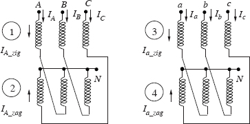
Figure 3.20 Zigzag/zigzag transformer.

The directions of the currents in the windings are shown in the figure. The per-unit ampere-turns on the limb corresponding to phase A are given as

$(I_{A_{-}zig}{)}^{\prime }=(I_{A_{-}zag}{)}^{\prime }=0.577\text{cos }30°$

$(I_{A_{-}zag}{)}^{″}=-(I_{A_{-}zig}{)}^{″}=0.577\text{sin }30°$

$(I_{a_{-}zig}{)}^{\prime }=(I_{a_{-}zag}{)}^{\prime }=0.577\text{cos }30°$

$(I_{a_{-}zig}{)}^{″}=-(I_{a_{-}zag}{)}^{″}=0.577\text{sin }30°.$

By using Equation 3.61, where n = 4 and remembering that I₁ = I_{A_zig}, I₂ = I_{A_zag}, I₃ = I_{a_zig}, I₄ = I_{a_zag}, we obtain

$\begin{array}{ll}Q=\hfill & \frac{-1}{2}\left\{\begin{array}{l}2X_{12}{I^{\prime }}_1{I^{\prime }}_2+2X_{13}{I^{\prime }}_1{I^{\prime }}_3+2X_{14}{I^{\prime }}_1{I^{\prime }}_4+2X_{23}{I^{\prime }}_2{I^{\prime }}_3\hfill \\ +2X_{24}{I^{\prime }}_2{I^{\prime }}_4+2X_{34}{I^{\prime }}_3{I^{\prime }}_4\hfill \end{array}\right\}\hfill \\ \hfill & \frac{-1}{2}\left\{\begin{array}{l}2X_{12}{I^{″}}_1{I^{″}}_2+2X_{13}{I^{″}}_1{I^{″}}_3+2X_{14}{I^{″}}_1{I^{″}}_4+2X_{23}{I^{″}}_2{I^{″}}_3\hfill \\ +2X_{24}{I^{″}}_1{I^{″}}_4+2X_{34}{I^{″}}_3{I^{″}}_4\hfill \end{array}\right\}.\hfill \end{array}$

After substituting the values of in-phase and quadrature components of I₁, I₂, I₃ and I₄ obtained earlier, we have

$Q=X_{Zigza{g}_{-}zigzag}=\frac{1}{3}\left[X_{13}+X_{24}+\left(\frac{X_{14}+X_{23}}{2}\right)-\left(\frac{X_{12}+X_{34}}{2}\right)\right].$

(3.64)

3.7    Zero-Sequence Reactances

The theory of symmetrical components is commonly used in power system analyses. Unlike in rotating machines, the positive-sequence and negative-sequence reactances are equal in static devices such as transformers. Under symmetrical loading conditions, only positive-sequence reactances need to be considered. During asymmetrical loadings/disturbances or single-phase faults, the response of the system is mainly decided by zero-sequence reactances in the resultant network. It is relatively easy to understand and calculate positive-sequence reactances as compared to zero-sequence reactances in transformers. The zero-sequence reactance of a transformer may differ considerably from its positive-sequence reactance depending upon the type of its magnetic circuit and winding connections.

The zero-sequence reactance seen from the terminals of a delta-connected winding is infinite, since zero-sequence currents cannot flow as there is no return path; the zero-sequence test will in fact measure a high capacitive reactance between the three phases and the ground (i.e., the winding to ground stray capacitances of the three phases are in parallel under the test condition).

In order to measure the zero-sequence reactance of a transformer having a star-connected winding, a suitable voltage is applied between the short-circuited line terminals of the winding and the neutral as shown in Figure 3.21. The zero-sequence reactance (≅ impedance) of the star-connected winding with the grounded neutral is calculated as

$X_0=\frac{V}{(I/3)}=3\frac{V}{I}.$

(3.65)

Two types of zero-sequence reactances can be measured for a winding:

1.  The open-circuit or magnetizing reactance with terminals of all other windings kept open-circuited

2.  The short-circuit or leakage reactance with terminals of only one other winding short-circuited.

The influence of the type of the core construction and winding connections on these reactances and the procedures for their calculation are now discussed.

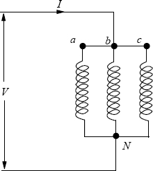
Figure 3.21 Measurement of zero-sequence impedance.

3.7.1    Open-circuit zero-sequence reactance without delta winding

A. Three-phase three-limb transformers

For a three-phase three-limb transformer, since the zero-sequence fluxes in the three limbs are in the same direction, they have to return through a path outside the core. In this case, the tank acts as an equivalent delta winding, and the open-circuit zero-sequence reactance is the one between the tank and the excited winding. Since the gap/area between the excited winding and the tank is much higher than the gap/area between the LV and HV windings, the open-circuit zero-sequence reactance is considerably higher than the short-circuit positive-sequence reactance (the usual leakage impedance between the windings), although it is much lower than the open-circuit positive sequence reactance obtained by the standard open-circuit test discussed in Chapter 1. The tank influences the zero-sequence reactance in the following way. It provides a lower reluctance return path (as compared to air) to the zero-sequence flux, which has the effect of increasing the reactance; on the other hand the tank enclosing the three phases acts as a short-circuited winding reducing the reactance. The latter effect is more dominant and hence the zero-sequence reactance inside the tank is appreciably less than that without it [15]. However, the zero-sequence reactance is much larger than the positive-sequence impedance as mentioned earlier.

The reactance between the excited winding and the tank can be calculated by the procedure given in Section 3.1.1 with the latter represented as an equivalent (fictitious) winding with zero radial depth (contribution of the tank to the AT diagram area can be neglected due to its small thickness). The winding-tank gap can be taken as the equivalent distance which gives approximately the same area of the space between them. The zero-sequence reactance is then calculated by using Equation 3.16 as

$\%X_0=2.48\times {10}^{-5}f\frac{(Ampere\times Turns)}{H_{eq}\times (Volts/Turn)}\times (\frac{1}{3}\times T_w\times D_w+T_g\times D_g)$

(3.66)

where

Tw	=	radial depth of the excited winding in cm
Dw	=	mean diameter of the excited winding in cm
Tg	=	gap between the excited winding and the tank in cm
Dg	=	mean diameter of the gap between the excited winding and the tank in cm.

When sufficient voltage is applied during the test, the zero-sequence flux passing through the tank usually saturates it. If the test is done at a voltage magnitude which does not saturate the tank made generally from mild steel material, its higher permeability will increase the reactance. Hence, the reactance calculated using Equation 3.66 has to be suitably corrected by an empirical factor which can be derived based on a set of measurements at various voltage levels. The correction factor depends on the applied voltage as shown in Figure 3.22 [16]. The curve in the figure has the same nature as that of the permeability versus magnetic field intensity graph derived from the measurements on a typical grade of mild steel material (Figure 3.23) [17].

B. Three-phase five-limb and single-phase three-limb transformers

In a three-phase five-limb transformer, the zero-sequence flux has a return path through the end yokes and the end limbs, and hence the open-circuit zero-sequence reactance equals the open-circuit positive-sequence reactance (a high value) unless the voltage applied is such that the yokes and the end limbs saturate. For an applied zero-sequence voltage close to the rated value of the excited winding, the yokes and the end limbs will be completely saturated; their area is too less to carry the zero-sequence flux of all the three phases at the rated voltage. This results in a lower value of the open-circuit zero-sequence reactance, which can be close to that for the three-phase three-limb construction.

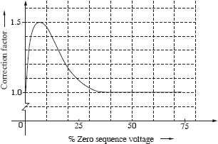
Figure 3.22 Correction factor for the zero-sequence reactance [16].

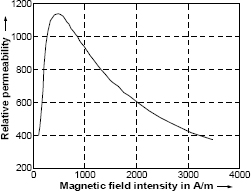
Figure 3.23 Variation of μ_r with field intensity in mild steel material [17].

For single-phase three-limb transformers, since the zero-sequence flux returns through the end limbs, the open-circuit zero-sequence reactance is equal to the open-circuit positive-sequence reactance (∼ infinite value). Thus, for a bank of three single-phase transformers, the zero-sequence characteristics are usually identical to the positive-sequence characteristics [18].

3.7.2    Open-circuit zero-sequence reactance with a delta-connected winding

With one delta connected secondary winding, a zero-sequence current circulates in the closed delta. Thus, the transformer acts as if it is short-circuited regardless of whether the winding is loaded or not. Let us again consider the following two cases.

A. Three-phase three-limb transformers

When zero-sequence voltage is applied to the star-connected winding, zero-sequence currents flow in the delta-connected winding and the tank which acts as an equivalent short-circuited (delta) winding. In order to estimate the current division between these two windings and the zero-sequence reactance, we will use the method described in Section 3.2 for a composite system of windings. Let the star-connected primary winding, the delta connected secondary winding and the tank be represented by notations 1, 2, and 3 respectively. Applying Equation 3.38, for the present case of the three windings (one star- and two delta-connected windings), we obtain the per-unit value of zero-sequence reactance as

$Q=X_0=-\frac{1}{2}\left[2X_{12}{I}_1(-I_2)+2X_{23}(-I_2)(-I_3)+2X_{13}{I}_1(-I_3)\right].$

(3.67)

The currents in windings 2 and 3 are assigned a negative sign as their direction is opposite to that of the current in the primary winding. Since the magnetizing current can be neglected,

$I_1=I_2+I_3.$

(3.68)

If the magnitude of the applied zero-sequence voltage is such that the rated current flows in the primary winding (i.e., I₁ has a value of 1 per-unit), then

$I_3=1-I_2.$

(3.69)

$\therefore Q=X_{12}{I}_2-X_{23}{I}_2(1-I_2)+X_{13}(1-I_2).$

(3.70)

The currents are distributed in the windings in such a way that the total energy is minimized. Hence, differentiating Q with respect to I₂ and equating the derivative to zero, we have

$\frac{dQ}{d{I}_2}=X_{12}-X_{23}+2X_{23}{I}_2-X_{13}=0.$

(3.71)

$\therefore I_2=\frac{X_{13}+X_{23}-X_{12}}{2X_{23}}.$

(3.72)

The above value of I₂ when substituted in Equation 3.69 gives the current flowing through the tank as

$I_3=\frac{X_{23}+X_{12}-X_{13}}{2X_{23}}.$

(3.73)

The delta-connected secondary winding can either be the inner or outer winding.

If the delta-connected winding (2) is the outer winding:

$X_{13}\cong X_{12}+X_{23}.$

(3.74)

Substituting the expression of X₁₃ in Equations 3.72 and 3.73, we obtain

$\begin{array}{ccc}{I}_2\cong 1& \text{and}& I_3\cong 0.\end{array}$

(3.75)

Substituting these values of I₂ and I₃ in Equation 3.70, the value of zero-sequence reactance is obtained as

$X_0=Q\cong X_{12}.$

(3.76)

Thus, with the outer delta-connected winding, the zero-sequence reactance is approximately equal to the short-circuit positive-sequence reactance (X₁₂) because the outer delta-connected winding shields the tank and no current flows in the latter. The phenomenon can be understood by referring to Figure 5.38 (a) wherein the leakage field is constrained to return through the limb to make the total flux linked to the outer short-circuited winding equal to zero.

If the delta-connected winding (2) is the inner winding:

$X_{23}\cong X_{21}+X_{13}=X_{12}+X_{13}.$

(3.77)

Substituting this expression of X₂₃ in Equations 3.72 and 3.73, we obtain

$\begin{array}{ccc}{I}_2\cong \frac{X_{13}}{X_{23}}& \text{and}& I_3\cong \frac{X_{12}}{X_{23}}.\end{array}$

(3.78)

Putting these expressions I₂ and I₃ in Equation 3.70, we have

$X_0=Q\cong \frac{X_{13}}{X_{23}}{X}_{12}.$

(3.79)

Thus, with the inner delta-connected winding, the zero-sequence reactance is always less than the (short-circuit) positive-sequence reactance (X₁₂). This is due to the fact that, in this case, X₂₃ > X₁₃ since the outer star-connected winding (1) is closer to the tank. In this case, as the effect of the tank is not hampered, the reactance reduces; the presence of an additional short-circuited winding has the effect of reducing the impedance seen from the source end in any system of windings.

It should to be noted that Equations 3.74 and 3.77 are approximately valid; for accurate calculations, the expressions of I₂ and I₃ in Equations 3.72 and 3.73, respectively, have to be directly substituted in Equation 3.70.

The value of the measured positive-sequence impedance is the same irrespective of which winding is excited. However, as discussed in this section, the measured zero-sequence impedance depends on whether the inner or outer winding is excited. For this reason, the zero-sequence tests are not reciprocal for three-phase three-limb units.

B. Three-phase five-limb and single-phase three-limb transformers

For a three-phase five-limb transformer, the value of zero-sequence reactance is equal to that of the short-circuit positive-sequence reactance between the windings until the applied voltage saturates the yokes and the end limbs. At such a high applied voltage, it acts as a three-limb transformer, and the zero-sequence reactance can be calculated accordingly.

For a single-phase three-limb transformer, the zero-sequence reactance is equal to the short-circuit positive-sequence reactance between the star- and delta-connected windings, since a current flows in the closed delta (as if short-circuited) and a path is available for the flux in the magnetic circuit.

Example 3.5

Calculate the positive-sequence and zero-sequence reactances of a 2 MVA, 11/0.433 kV, 50 Hz, Dyn11 transformer whose various relevant dimensions in mm are indicated in Figure 3.24. The value of volts/turn is 15.625.

Solution:

The short-circuit positive-sequence (leakage) reactance is calculated by the procedure given in Section 3.1.1 for concentric windings.

The Rogowski factor is calculated by Equation 3.18 as

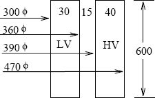
Figure 3.24 Dimensions of 2 MVA transformer.

$K_R=1-\frac{1-e^{-\pi 60.0/(3.0+1.5+4.0)}}{\pi 60.0/(3.0+1.5+4.0)}=\mathrm{0.955.}$

The equivalent winding height according to Equation 3.1 is

H_eq = H_w / K_R = 60 / 0.955 = 62.8.

${\displaystyle \sum ATD}$ is calculated using Equation 3.17,

${\displaystyle \sum ATD=\frac{1}{3}\times 3.0\times 33.0+1.5\times 37.5+\frac{1}{3}\times 4.0\times 43.0=\mathrm{146.6.}}$

For calculating the reactance, either the LV or HV ampere-turns are used (their values are equal since the magnetizing ampere-turns are neglected).

$\text{LV current}=\frac{2\times {10}^6}{\sqrt{3}\times 433}=2666.67\text{A and LV tums}=\frac{433/\sqrt{3}}{15.625}=16.$

The positive-sequence leakage reactance is given by Equation 3.16,

$\%X_p=2.48\times {10}^{-5}\times 50\times \frac{(2666.67\times 16)}{62.8\times 15.625}\times 146.6=7.9\%.$

Since the delta-connected HV winding is the outer winding, the zero-sequence reactance of the star-connected winding is approximately equal to the positive-sequence leakage reactance as explained in Section 3.7.2. However, during the actual test, one usually gets the value of zero-sequence reactance higher than the positive-sequence leakage reactance by an amount corresponding to the voltage drop in the neutral bar. The reactance of a neutral bar having rectangular dimensions (a × b) is given by the expression [19, 20]:

$X_n=2\pi f\times 0.002L_b\left\{{\text{log}}_e\frac{2L_b}{D_s}-1+\frac{D_s}{L_b}\right\}\times {10}^{-6}$

(3.80)

where

L_b is the length of the bus-bar in cm, and

D_s is the geometric mean distance from itself = 0.2235× (a + b) cm.

For the bus-bar dimensions, a = 5 cm, b = 0.6 cm, length = 50 cm,

$D_s=0.2235\times (5+0.6)=\mathrm{1.2516.}$

$\begin{array}{l}\therefore X_n=2\pi \times 50\times 0.002\times 50\times \left\{{\text{log}}_e\frac{2\times 50}{1.2516}-1+\frac{1.2516}{50}\right\}\times {10}^{-6}\\ =107\times {10}^{-6}\text{Ω}.\end{array}$

The base impedance on the LV side is

$Z_b=\frac{{(0.433)}^2}{2}=\mathrm{0.0937.}$

Since the zero-sequence current flowing in the neutral bar is three times that flowing in each of the phases, the bar contributes three times the value of X_n in zero-sequence reactance.

$\therefore \%X_n=\frac{3\times 107\times {10}^{-6}}{0.0937}\times 100=0.34\%.$

Hence, the measured zero-sequence reactance would be close to

${(X_0)}_{actual}=7.9+0.34=8.24\%.$

3.7.3    Short-circuit zero-sequence reactance

This is applicable when the secondary winding is short-circuited while doing the zero-sequence test on the primary winding (e.g., a star/star transformer).

A. Three-phase three-limb transformers

The procedure for the calculation of the short-circuit zero-sequence reactance of three-phase three-limb transformers is now explained with the help of an example.

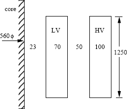
Figure 3.25 Dimensions of the transformer in Example 3.6.

Example 3.6

The relevant dimensions (in mm) of a 31.5 MVA, 132/33 kV, 50 Hz, YNyn transformer are given in Figure 3.25. The volts/turn is 83.93. Calculate the zero-sequence reactance of the LV and HV windings, and the parameters of the zero-sequence network.

Solution:

The value of the positive-sequence leakage reactance can be calculated like in the previous examples as 12.16%. Let the inner 33 kV winding and the outer 132 kV winding be denoted by numbers 1 and 2 respectively.

X_p = (X_p)₁₂ = (X_p)₂₁ = 12.16%.

The open-circuit zero-sequence reactance of the LV and HV windings can be calculated by using the procedure given in Section 3.7.1 (and Equation 3.66) with the average LV-to-tank and HV-to-tank distances of 400 mm and 250 mm (for this transformer) respectively. Let us first calculate the open-circuit reactance as seen from the LV winding.

$\begin{array}{cccccc}{T}_1=7\text{cm,}& T_g=40\text{cm},& T_2\approx 0,& H_w=125\text{cm},& K_R=0.88,& H_{eq}=142\text{cm,}\end{array}$

$\text{HV}\text{current}\text{=}\text{137}\text{.78}\text{A,}$

$\text{HV}\text{turns}=\frac{132\times {10}^3/\sqrt{3}}{83.93}=908,$

$\begin{array}{l}{\left(X_z\right)}_{1_{-}oc}=\frac{2.48\times {10}^{-5}\times 50\times \left(137.78\times 908\right)}{142\times 83.93}\times \left(\frac{1}{3}\times 7.0\times 67.6+40\times 114.6\right)\hfill \\ =61.73\%.\hfill \end{array}$

Similarly,

$\begin{array}{l}{\left(X_z\right)}_{2_{-}oc}=\frac{2.48\times {10}^{-5}\times 50\times \left(137.78\times 908\right)}{137.2\times 83.93}\times \left(\frac{1}{3}\times 10\times 94.6+25\times 129.6\right)\hfill \\ =49.89\%\hfill \end{array}$

The zero-sequence reactance as seen from the inner LV winding with the outer HV winding short-circuited is the same as the positive-sequence leakage reactance (if the reactance contributed by the neutral bar is neglected),

${(X_z)}_{{12}_{-}sc}=X_p=12.16\%.$

The zero-sequence reactance as seen from the HV winding with the LV winding short-circuited is calculated using Equation 3.79,

${(X_z)}_{{21}_{-}sc}=X_p\times \frac{{(X_z)}_{2_{-}oc}}{{(X_z)}_{1_{-}oc}}=12.16\times \frac{47.89}{61.73}=9.44\%.$

The zero-sequence network [18] of this two winding transformer is shown in Figure 3.26 which satisfies all the calculated zero-sequence reactance values, (X_z)_{1 _ oc}, (X_z)_{2 _ oc}, (X_z)_{12 _ sc} and (X_z)_{21 _ sc}.

For example, the zero-sequence reactance as seen from the (excited) HV winding with the short-circuited LV winding is

${(X_z)}_{{21}_{-}sc}=-0.835+(13.0\text{//}48.73)=-0.835+\frac{13.0\times 48.73}{13.0+48.73}=9.43\%,$

which matches closely with the value calculated previously.

In a similar way, the zero-sequence reactance of a three-winding three-phase three-limb transformer can be estimated as demonstrated by the following example.

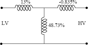
Figure 3.26 The zero-sequence network of the two-winding transformer in Example 3.6.

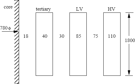
Figure 3.27 Dimensions of the three-winding transformer in Example 3.7.

Example 3.7

The relevant dimensions (in mm) of a 100 MVA, 220/66/11 kV, 50 Hz, YNynd1 transformer are given in Figure 3.27. The volts/turn is 160. Calculate the zero-sequence reactance of the transformer as seen from the HV winding with the LV winding short-circuited (and in the presence the delta-connected tertiary winding).

Solution:

Let the tertiary (11 kV), LV (66 kV) and HV (220 kV) windings be denoted by numbers 1, 2, and 3 respectively. The short-circuit positive-sequence reactances for the three pairs of the windings are calculated as

$\begin{array}{cccc}{(X_p)}_{12}=6.0\%,& {(X_p)}_{23}=14.6\%,& \text{and}& {(X_p)}_{13}=22.64\%.\end{array}$

The open circuit zero-sequence reactances of the tertiary, LV and HV windings with an average distance of 250 mm between the HV winding and the tank are calculated as

$\begin{array}{cccc}{(X_z)}_{1_{-}oc}=64.81\%,& {(X_z)}_{2_{-}oc}=57.71\%& \text{and}& {(X_z)}_{3_{-}oc}=40.93\%.\end{array}$

The various zero-sequence reactances between the pairs of the windings are now obtained using Equation 3.79:

1.  Zero-sequence voltage is applied to the HV winding, the LV winding is open-circuited, and the tertiary-delta is closed,

${(X_z)}_{{31}_{-}sc}=\frac{{(X_z)}_{3_{-}oc}}{{(X_z)}_{1_{-}oc}}\times {(X_p)}_{31}=\frac{40.93}{64.81}\times 22.64=14.3\%.$

2.  Zero-sequence voltage is applied to the LV winding, the HV winding is open-circuited, and the tertiary-delta is closed,

${(X_z)}_{{21}_{-}sc}=\frac{{(X_z)}_{2_{-}oc}}{{(X_z)}_{1_{-}oc}}\times {(X_p)}_{21}=\frac{57.71}{64.81}\times 6.0=5.34\%.$

3.  Zero-sequence voltage is applied to the HV winding, the LV winding is short-circuited, and the tertiary-delta is open,

${(X_z)}_{{32}_{-}sc}=\frac{{(X_z)}_{3_{-}oc}}{{(X_z)}_{2_{-}oc}}\times {(X_p)}_{32}=\frac{40.93}{57.71}\times 14.6=10.36\%.$

The zero-sequence reactances of the three windings can now be calculated by using equations given in Section 3.5,

${(X_z)}_1=\frac{1}{2}\times [{(X_z)}_{{21}_{-}sc}+{(X_z)}_{{31}_{-}sc}-{(X_z)}_{{32}_{-}sc}]=4.64\%$

${(X_z)}_2=\frac{1}{2}\times [{(X_z)}_{{21}_{-}sc}+{(X_z)}_{{32}_{-}sc}-{(X_z)}_{{31}_{-}sc}]=0.7\%$

${(X_z)}_3=\frac{1}{2}\times [{(X_z)}_{{31}_{-}sc}+{(X_z)}_{{32}_{-}sc}-{(X_z)}_{{21}_{-}sc}]=9.66\%.$

The zero-sequence star equivalent network of the three-winding transformer is shown in Figure 3.28. Using the network, the zero-sequence reactance of the transformer if measured from the HV side with the LV winding short-circuited and tertiary-delta closed can be determined as

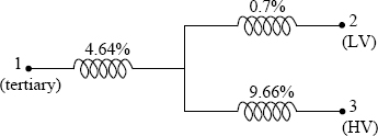
Figure 3.28 Zero-sequence star equivalent circuit.

${(X_z)}_{3_{-}21}=9.66+(0.7\text{//}4.64)=10.27\%.$

Here, the system of four windings (i.e., the tertiary, LV and HV windings plus an imaginary winding representing the currents flowing in the tank) is converted into the equivalent three-winding system which takes into account the effect of the tank while calculating the short-circuit zero-sequence reactance between any two of the tertiary, LV and HV windings. Hence, the calculation of (X_z)_{3 _ 21} by the star equivalent circuit of Figure 3.28 is an approximate way. Actually, the problem needs to be solved with an additional delta-connected winding representing the tank.

Let us now calculate the reactance by treating the tank as the fourth winding. The zero-sequence reactance can be calculated by the procedure given in Section 3.2 (i.e., the reactive kVA approach). Let I₁, I₂ and I₄ be the currents flowing through the tertiary, LV and equivalent delta (tank) windings respectively. The current flowing through the HV winding (I₃) is 1 per-unit and we know that

I₃ = 1 = I₁ + I₂ + I₄.

The expression for Q is

$Q=-\frac{1}{2}\left({}_{+2{(X_p)}_{23}(-I_2)I_3+2{(X_p)}_{24}(-I_2)(-I_4)+2{(X_p)}_{34}{I}_3(-I_4)}^{2{(X_p)}_{12}(-I_1)(-I_2)+2{(X_p)}_{13}(-I_1)I_3+2{(X_p)}_{14}(-I_1)(-I_4)}\right).$

The reactance between the tank and any other winding has already been calculated (e.g., (X_p)₁₄ = (X_z)_{1 _ oc} = 64.81 %). By putting the values of all the reactances and using I₁ = 1 − I₂ − I₄, the above expression becomes

$Q=\left(22.64-14.04I_2-46.52I_4+13.1I_2{I}_4+6I_2^2+64.81I_4^2\right).$

In order to have a minimum energy state, we differentiate the above expression with respect to I₂ and I₄, and equate the derivatives to zero and obtain two simultaneous equations. These two equations are solved to give

I₂ = 0.8747 and I₄ = 0.2705.

Putting these values in the expression for Q, we have (X_z)_{3 _ 21} = 10.21%, which is close to that calculated by using the star equivalent circuit (i.e., 10.27%).

The methods described for the calculation of zero-sequence reactances can give reasonably accurate results and should be refined by empirical correction factors, if required, based on the results of tests conducted on a number of transformers. For more accurate calculations, numerical methods like FEM can be used [21, 22], in which the effect of the tank saturation on the zero-sequence reactance can be exactly simulated. The tank material should be modeled by defining its conductivity and nonlinear B-H characteristics. In power transformers, tank shunts of a CRGO material are commonly put on the inner tank wall to reduce stray losses due to the leakage field. As explained earlier, the tank acts as an equivalent delta winding and reduces the zero-sequence reactance. The shunts provide an alternative low reluctance path to the zero-sequence flux and mitigate the effect of the tank. The magnetic shunts on the tank wall, therefore, have the effect of increasing the zero-sequence reactance. In such cases, an FEM analysis is essential for correct estimation of the reactance.

B. Three-phase five-limb and single-phase three-limb transformers

Since short-circuit reactances are much smaller than open-circuit reactances, the applied zero-sequence voltages, required to circulate rated currents, are usually much smaller than the rated voltages. Hence, in three-phase five-limb transformers, the yokes and the end limbs (which provide a path for the zero-sequence flux) do not saturate. Therefore, there will not be any currents flowing in the tank since all the flux is contained within the core. Hence, the short-circuit zero-sequence reactance is equal to the short-circuit positive-sequence reactance (the usual leakage reactance) in the three-phase five-limb transformers.

In single-phase three-limb transformers, their yokes and end limbs provide a path for the zero-sequence flux, and hence the zero-sequence reactance is equal to the positive-sequence reactance.

The above inferences can be drawn by analyzing the zero-sequence network in Figure 3.26. The shunt reactance is very high (∼ infinity) due to a low reluctance value of the path provided by the end limbs and yokes in single-phase three-limb and three-phase five-limb transformers; the shunt branch now represents the magnetizing reactance in place of the reactance representing the imaginary (short-circuited) tank winding. This makes the short-circuit zero-sequence reactance equal to the corresponding positive-sequence (leakage) reactance with the HV winding excited and the LV winding short-circuited (or with the LV winding excited and the HV winding short-circuited).

3.8    Stabilizing Tertiary Winding

As mentioned earlier, in addition to primary and secondary windings, transformers are many times provided with an additional tertiary winding. It can be used for the following purposes:

•  Static capacitors or synchronous condensers can be connected to the tertiary winding for injection of reactive power into the system for maintaining its voltage profile within certain limits.

•  Auxiliary equipment in the substation can be supplied at a voltage level which is different and lower than that of the primary and secondary windings.

•  Three windings may be required for interconnecting three transmission lines operating at different voltages.

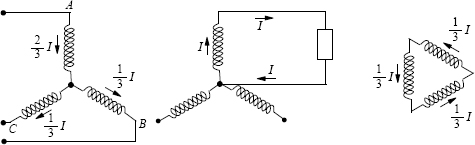
Figure 3.29 Unbalanced load.

In these applications, the tertiary winding (which may be a star- or a delta-connected winding) is loaded. Sometimes an additional delta-connected tertiary winding is provided in transformers with the star- or auto-star-connected primary and secondary windings, which is usually not designed to take any load. Such an unloaded delta-connected winding is used for the stabilizing purpose as described below.

•  Third harmonic magnetizing currents flow in the closed delta, making the induced voltages and the core flux almost sinusoidal (refer to Section 2.8).

•  The winding stabilizes the neutral point; the zero-sequence impedance is lower and an unbalanced load can be taken without creating an undue unbalance in the phase voltages. Under asymmetrical loading conditions, the currents flow in such a way that the ampere-turns of the three windings balance each other as shown in Figure 3.29 for the case of a single-phase loading condition. The load on each phase of the tertiary winding is one-third of the single-phase load. Hence, the rating of the tertiary winding is usually one-third of the rating of the main windings.

•  It can prevent the interference in telephone lines caused by third harmonic currents and voltages of transmission lines and earth circuits.

In the previous section, we have seen that the zero-sequence characteristics of three-phase three-limb transformers and three-phase five-limb transformers/banks of single-phase transformers are different. The magnetic circuit of the three-phase three-limb type acts as if open-circuited offering a high reluctance to the zero-sequence flux, and hence a lower zero-sequence reactance is obtained. It should be remembered that the higher the reluctance of a magnetic circuit the lower is the reactance reflected in its equivalent electric circuit. Three phase three-limb construction is not suitable for significantly unbalanced conditions since the resulting zero sequence flux has to complete its path through the tank structure which gets overheated due to induced eddy currents. The five-limb and the shell form constructions are better-suited for unbalanced operations, since there is a path for the zero-sequence flux in them.

The magnetic circuit of three-phase five-limb transformers/banks of single-phase transformers can be visualized as a closed one giving a very high value of the zero-sequence reactance. If a delta-connected stabilizing winding is added to these three types of transformers, three-phase three-limb transformers, banks of three single-phase three-limb transformers, and three-phase five-limb transformers, the difference between the zero-sequence reactance characteristics of the three-phase three-limb transformers and that of the other two types diminishes. As long as one delta-connected winding is present, it makes a very little difference whether it is an effectively open or closed magnetic circuit from the zero-sequence reactance point of view.

A frequently asked question is whether the stabilizing winding can be dispensed with in the three-phase three-limb star-star (or auto-star) connected transformers with the grounded neutral condition. This is because, as seen in the previous section, the high reluctance nonmagnetic path offered to the zero-sequence flux results in a lower zero-sequence reactance as compared to the positive-sequence reactance, and thus to some extent the effect of the stabilizing winding is achieved. Whether or not the stabilizing winding can be omitted depends mainly on whether the zero-sequence and third harmonic characteristics are compatible with the system into which the transformer is going to be installed. If these two characteristics are not adversely affected in the absence of the stabilizing winding, it may be omitted [23]. Away from distribution points, in transmission networks the loading of the three phases of transformers is more or less balanced. Also, if the telephone-interference problem due to harmonic currents is within limits, and if the zero-sequence currents during asymmetrical fault conditions are large enough to be easily detected, the provision of the stabilizing winding in the three-phase three-limb transformers can be reviewed. This is because, since the stabilizing winding is generally unloaded, its conductor dimensions tend to be smaller. Such a winding becomes weak and vulnerable under asymmetrical fault conditions, which is a subject of discussion in Chapter 6.

Consequences of omitting the stabilizing winding in banks of three single-phase transformers/three-phase five-limb transformers can be significant. The zero-sequence reactance will be higher, and if the disadvantages of its high value cannot be tolerated, the stabilizing winding cannot be omitted. A low voltage stabilizing winding, with its terminal brought out, helps in very large transformers for carrying out tests such as the no-load loss test in the manufacturer’s works. In the absence of this winding, it may not be possible to do the test if the manufacturer does not have a high-voltage source or a suitable step-up transformer. Alternatively, a star-connected auxiliary winding can be provided for the testing purpose, whose terminals can be buried inside the tank after the testing.

References

1.    Blume, L. F., Boyajian, A., Camilli, G., Lennox, T. C., Minneci, S., and Montsinger, V. M. Transformer engineering, John Wiley and Sons, New York, and Chapman and Hall, London, 1951.

2.    Hayt, W. H. Engineering electromagnetics, McGraw-Hill Book Company, Singapore, 1989, pp. 298–301.

3.    Garin, A. N. and Paluev, K. K. Transformer circuit impedance calculations, AIEE Transactions — Electrical Engineering, June 1936, pp. 717–729.

4.    Waters, M. The short circuit strength of power transformers, Macdonald, London, 1966, pp. 24–25, p. 53.

5.    Boyajian, A. Leakage reactance of irregular distributions of transformer windings by method of double Fourier series, AIEE Transactions — Power Apparatus and Systems, Vol. 73, Pt. III-B, 1954, pp. 1078–1086.

6.    Sollergren, B. Calculation of short circuit forces in transformers, Electra, Report no. 67, 1979, pp. 29–75.

7.    Rabins, L. Transformer reactance calculations with digital computers, AIEE Transactions — Communications and Electronics, Vol. 75, Pt. I, 1956, pp. 261–267.

8.    Silvester, P. P. and Ferrari, R. L. Finite elements for electrical engineers, Cambridge University Press, New York, 1990.

9.    Andersen, O. W. Transformer leakage flux program based on Finite Element Method, IEEE Transactions on Power Apparatus and Systems, Vol. PAS-92, 1973, pp. 682–689.

10.  Rothe, P. S. An introduction to power system analysis, John Wiley and Sons, New York, 1953, pp. 45–50.

11.  Boyajian, A. Theory of three-circuit transformers, AIEE Transactions, February 1924, pp. 508–528.

12.  Starr, F. M. An equivalent circuit for the four-winding transformer, General Electric Review, Vol. 36, No. 3, March 1933, pp. 150–152.

13.  Aicher, L. C. Useful equivalent circuit for a five-winding transformer, AIEE Transactions — Electrical Engineering, Vol. 62, February 1943, pp. 66–70.

14.  Schaefer, J. Rectifier circuits: theory and design, John Wiley and Sons, New York, 1965, pp. 12–19.

15.  Christoffel, M. Zero-sequence reactances of transformers and reactors, The Brown Boveri Review, Vol. 52, No. 11/12, November/December 1965, pp. 837–842.

16.  Clarke E. Circuit analysis of AC power systems, Vol. II, John Wiley and Sons, New York, Chapman and Hall, London, 1957, p. 153.

17.  Jha, S. K. Evaluation and mitigation of stray losses due to high current leads in transformers, M. Tech Dissertation, Department of Electrical Engineering, IIT-Bombay, India, 1995.

18.  Garin, A. N. Zero phase sequence characteristics of transformers, General Electric Review, Vol. 43, No. 3, March 1940, pp. 131–136.

19.  Copper Development Association, Copper for busbars, Publication No. 22, January 1996, p. 53.

20.  Schurig, O. R. Engineering calculation of inductance and reactance for rectangular bar conductors, General Electric Review, Vol. 36, No. 5, May 1933, pp. 228–231.

21.  Allcock, R., Holland, S., and Haydock, L. Calculation of zero phase sequence impedance for power transformers using numerical methods, IEEE Transactions on Magnetics, Vol. 31, No. 3, May 1995, pp. 2048–2051.

22.  Ngnegueu, T., Mailhot, M., Munar, A., and Sacotte, M. Zero phase sequence impedance and tank heating model for three-phase three-leg core type power transformers coupling magnetic field and electric circuit equations in a Finite Element software, IEEE Transactions on Magnetics, Vol. 31, No. 3, May 1995, pp. 2068–2071.

23.  Cogbill, B. A. Are stabilizing windings necessary in all Y-connected transformers, AIEE Transactions — Power Apparatus and Systems, Vol. 78, Pt. 3, 1959, pp. 963–970.