4

Eddy Currents and Winding Stray Losses

The load loss of a transformer consists of the loss due to the ohmic resistance of windings (I²R losses) and some additional losses. These additional losses are generally known as stray losses which occur due to the leakage field of windings and the field of high current carrying leads/bus-bars. The stray losses in the windings are further classified as eddy and circulating current losses. The remaining stray losses occur in structural steel parts. There is always some amount of leakage field in all types of transformers, and in large power transformers, which may be limited in size due to transport and space restrictions, the stray field strength increases with the rating much faster than in small transformers. The stray flux impinging on conducting parts (winding conductors and structural components) induces eddy currents in them. The stray loss in windings can be substantially high in large transformers if conductor dimensions and transposition methods are not chosen properly.

Today’s designer faces challenges like higher loss capitalization rates and optimum performance requirements. In addition, there could be constraints on the dimensions and weight of the transformer. If the designer lowers the current densities in the windings to reduce the DC resistance loss (i.e., the I²R loss), the eddy loss in them increases due to increased conductor dimensions. Hence, the winding conductors are usually subdivided using a proper transposition method to minimize the stray loss.

In order to accurately estimate and control the stray losses in windings and structural parts, an in-depth understanding of the fundamentals of eddy currents is desirable. Hence, the theory of eddy currents is described in the initial part of this chapter. The eddy loss and circulating current loss in windings are analyzed in subsequent sections. Methods for the evaluation and control of these two losses are also described. The remaining components of the stray losses that occur in structural components are elaborated in Chapter 5.

4.1    Field Equations

The differential forms of Maxwell’s equations, valid for static as well as time-dependent fields and also for free space as well as material bodies, are

$\nabla \times E=-\frac{\partial B}{\partial t}$

(4.1)

$\nabla \times H=J+\frac{\partial D}{\partial t}$

(4.2)

$\nabla \cdot B=0$

(4.3)

$\nabla \cdot D=\rho$

(4.4)

where H	= magnetic field strength (A/m)
E	= electric field strength (V/m)
B	= flux density (Wb/m2)
J	= current density (A/m2)
D	= electric flux density (C/m2)
ρ	= volume charge density (C/m3).

There are three constitutive relations,

$J=\sigma E$

(4.5)

$B=\mu H$

(4.6)

$D=\epsilon E$

(4.7)

where μ	= permeability of material (henrys/m)
ε	= permittivity of material (farads/m)
σ	= conductivity (mhos/m).

The ratio of the conduction current density (J) to the displacement current density (∂D/∂t) is given by the ratio σ/(jωε), which is very high even for a poor metallic conductor (where ω is frequency in rad/sec). Since our analysis is for the power frequency, the displacement current density is neglected for the analysis of eddy currents in the conducting parts of transformers (copper, aluminum, steel, etc.). Hence, Equation 4.2 is simplified to

$\nabla \times H=J.$

(4.8)

The principle of conservation of charge gives the point form of the continuity equation,

$\nabla \cdot J=-\frac{\partial \rho }{\partial t}.$

(4.9)

For slow time-varying fields in the present analysis of eddy currents in a conductor, displacement currents are neglected:

$\nabla \cdot J=0.$

(4.10)

The first-order differential Equations 4.1 and 4.8 involving both H and E are combined to give a second-order equation in H or E as follows. Taking the curl of both sides of Equation 4.8 and using Equation 4.5 we obtain,

$\nabla \times \nabla \times H=\nabla \times \sigma E.$

For a constant value of conductivity (σ), using vector algebra the equation can be simplified as

$\nabla (\nabla \cdot H)-{\nabla }^{2}H=\sigma \nabla \times E.$

(4.11)

Using Equation 4.6, with linear magnetic characteristics (i.e., constant μ), Equation 4.3 can be rewritten as

$\nabla \cdot B=\nabla \cdot \mu H=\mu \nabla \cdot H=0$

(4.12)

which gives

$\nabla \cdot H=0.$

(4.13)

Using Equations 4.1 and 4.13, Equation 4.11 is simplified to

${\nabla }^{2}H=\sigma \frac{\partial B}{\partial t}$

(4.14)

or

${\nabla }^{2}H-\mu \sigma \frac{\partial H}{\partial t}=0$

(4.15)

which is known as a diffusion equation. Now, in the frequency domain, Equation 4.1 can be written as follows (the field quantities are phasors as well; caps are not put on their top for brevity):

$\nabla \times E=-j\omega B$

(4.16)

where the term jω appears because the partial derivative of a sinusoidal field quantity with respect to time is equivalent to multiplying the corresponding phasor by jω. Using Equation 4.6 we have

$\nabla \times E=-j\omega \mu H.$

(4.17)

Taking the curl of both sides of the equation,

$\nabla \times \nabla \times E=-j\omega \mu \nabla \times H.$

(4.18)

Using Equation 4.8 we obtain

$\nabla \times \nabla \times E=-j\omega \mu J.$

(4.19)

Following the steps similar to those used for arriving at the diffusion Equation 4.15 and using the fact that ∇ · E = (1/ε) ∇ · D = ρ/ε = 0 (since no volume charge density is present) we have

$\nabla \times \nabla \times E=-{\nabla }^{2}E=-j\omega \mu J.$

(4.20)

Substituting the value of J from Equation 4.5,

${\nabla }^{2}E=j\omega \mu \sigma E.$

(4.21)

Now, let us assume that the vector field E has component only along the x axis.

$\therefore {\nabla }^2{E}_x=j\omega \mu \sigma E_x.$

(4.22)

The expansion of the operator ∇ leads to a second-order partial differential equation,

$\frac{{\partial }^2{E}_x}{\partial x^2}+\frac{{\partial }^2{E}_x}{\partial y^2}+\frac{{\partial }^2{E}_x}{\partial z^2}=j\omega \mu \sigma E_x.$

(4.23)

Suppose, if we further assume that E_x is a function of z only (i.e., it does not vary with x and y), then Equation 4.23 reduces to the following ordinary differential equation,

$\frac{d^2{E}_x}{d{z}^2}=j\omega \mu \sigma E_x.$

(4.24)

We can write the solution of Equation 4.24 as

$E_x=E_{xp}{e}^{-\gamma z}+E_{xp}{e}^{+\gamma z}$

(4.25)

where E_xp is the amplitude factor, and γ is the propagation constant which can be expressed in terms of the attenuation constant α and the phase constant β,

$\gamma =\alpha +j\beta .$

(4.26)

Substituting the value of E_x from Equation 4.25 in Equation 4.24 we obtain

$E_{xp}{\gamma }^2{e}^{-\gamma z}+E_{xp}{\gamma }^2{e}^{+\gamma Z}=j\omega \mu \sigma (E_{xp}{e}^{-\gamma z}+E_{xp}{e}^{+\gamma z}),$

(4.27)

which results in

${\gamma }^2=j\omega \mu \sigma .$

(4.28)

$\therefore \gamma =\pm \sqrt{j\omega \mu \sigma }.$

(4.29)

If the field E_x is incident on a surface of a conductor at z = 0 and is attenuated inside the conductor (z > 0), then only the plus sign has to be taken for γ.

$\therefore \gamma =\sqrt{j\omega \mu \sigma }=\sqrt{\omega \mu \sigma }\times \sqrt{1\angle {90}^{°}}=\sqrt{\omega \mu \sigma }\times 1\angle {45}^{°}.$

(4.30)

$\therefore \gamma =(1+j)\sqrt{\frac{\omega \mu \sigma }{2}}.$

(4.31)

Substituting ω = 2π f, we obtain

$\gamma =(1+j)\sqrt{\pi f\mu \sigma }.$

(4.32)

Hence,

$\alpha =\beta =\sqrt{\pi f\mu \sigma }.$

(4.33)

The electric field intensity in the complex exponential notation in Equation 4.25, which is assumed to be along the x axis and is traveling or penetrating inside the conductor in +z direction, becomes

$E_x=E_{xp}{e}^{-\gamma z}$

(4.34)

which in the time domain can be written as

$E_x=E_{xp}{e}^{-\alpha z}\text{ cos }(\omega t-\beta z).$

(4.35)

Substituting the values of α and β from Equation 4.33, we obtain

$E_x=E_{xp}{e}^{-z\sqrt{\pi f\mu \sigma }}\text{ cos }(\omega t-z\sqrt{\pi f\mu \sigma }).$

(4.36)

The conductor surface is represented by z = 0. Let z > 0 and z < 0 represent the regions corresponding to the conductor and the loss-free dielectric medium respectively. The source field at the surface of the conductor which establishes fields in it is

${(E_x)}_{z=0}=E_{xp}\text{ cos }\omega t.$

Making use of Equation 4.5, which says that the current density within a conductor is directly related to the electrical field intensity, we can write

$J_x=\sigma E_x=\sigma E_{xp}{e}^{-z\sqrt{\pi f\mu \sigma }}\text{ cos }(\omega t-z\sqrt{\pi f\mu \sigma }).$

(4.37)

Equations 4.36 and 4.37 tell us that away from the source at the surface and with penetration into the conductor, there is an exponential decrease in the electric field intensity and the conduction current density. At a distance of penetration $z=1/\sqrt{\pi f\mu \sigma }$, the exponential factor becomes e⁻¹(= 0.368), indicating that the value of the field (at this distance) reduces to 36.8% of that at the surface. This distance is called as the skin depth or the depth of penetration,

$\delta =\frac{1}{\sqrt{\pi f\mu \sigma }}=\sqrt{\frac{2}{\omega \mu \sigma }}.$

(4.38)

All the fields at the surface of a good conductor decay rapidly as they penetrate a few skin depths into it. Comparing Equations 4.33 and 4.38, we obtain the relationship,

$\begin{array}{ccc}\delta =\frac{1}{\alpha }=\frac{1}{\beta }& \text{and}& \gamma =\alpha +j\beta =\frac{1}{\delta }+\frac{j}{\delta }=(1+j)\times \frac{1}{\delta }\end{array}.$

(4.39)

The skin depth is a very important parameter in describing the behavior of a conductor subjected to electromagnetic fields. The conductivity of copper conductor at 75°C (the temperature at which the load loss of transformers is usually calculated and guaranteed) is 4.74 × 10⁷ mhos/m. Copper, being a non-magnetic material, has relative permeability of 1. Hence, the skin depth of copper at the power frequency of 50 Hz is

${\delta }_{Cu}=\frac{1}{\sqrt{\pi \times 50\times {\mu }_0{\mu }_r\times \sigma }}=\frac{1}{\sqrt{\pi \times 50\times 4\pi \times {10}^{-7}\times 1\times 474\times {10}^7}}=0.0103\text{m}$

or 10.3 mm. The corresponding value at 60 Hz is 9.4 mm. For aluminum, whose conductivity is approximately 61% that of copper, the skin depth at 50 Hz is 13.2 mm. Most of the structural elements inside a transformer are made of either mild steel (MS) or stainless steel (SS) material. For a typical grade of MS material with relative permeability of 100 (assuming that it is saturated) and conductivity of 7 × 10⁶ mho/m, the skin depth is δ_MS = 2.69 mm at 50 Hz. Non-magnetic stainless steel is commonly used for structural components in the vicinity of fields due to high currents. For a typical grade of SS material with relative permeability of 1 (non-magnetic) and conductivity of 1.136 × 10⁶ mho/m, the skin depth is δ_SS = 66.78 mm at 50 Hz.

4.2    Poynting Vector

Poynting’s theorem is the expression of the law of conservation of energy applied to electromagnetic fields. When the displacement current is neglected, as in the previous section, Poynting’s theorem can be mathematically expressed as [1, 2]

$-{\displaystyle \underset{s}{\oint }(E\times H)\cdot n\text{d}s={\displaystyle \underset{vs}{\int }H\cdot \frac{\partial B}{\partial t}\text{d}v}+{\displaystyle \underset{v}{\int }J\cdot E\text{d}v}}$

(4.40)

where v is the volume enclosed by the surface s and n is the unit vector normal to the surface directed outwards. Using Equation 4.5, the above equation can be modified as

$-{\displaystyle \underset{s}{\oint }(E\times H)\cdot n\text{d}s={\displaystyle \underset{vs}{\int }H\cdot \frac{\partial B}{\partial t}\text{d}v}+\frac{1}{\sigma }{\displaystyle \underset{v}{\int }{\left|J\right|}^2\text{d}v}.}$

(4.41)

This is a simpler form of Poynting’s theorem which states that the net inflow of power is equal to the sum of the power absorbed by the magnetic field and the ohmic loss. The Poynting vector is given by the vector product,

$P=E\times H$

(4.42)

which expresses the instantaneous density of power flow at a point.

Now, with E having only an x component which varies as a function of z only, Equation 4.17 becomes

$\begin{array}{ccc}\frac{\partial E_x}{\partial z}=-j\omega \mu H_y,& H_x=0,& H_Z=0.\end{array}$

(4.43)

Substituting the value of E_x from Equation 4.34 and rearranging we obtain

$H_y=\frac{1}{-j\omega \mu }\times \frac{\partial }{\partial z}(E_{xp}{e}^{-\gamma z})=\frac{\gamma E_x}{j\omega \mu }$

(4.44)

The ratio of E_x to H_y is defined as the intrinsic impedance,

$\eta =\frac{E_x}{H_y}=\frac{j\omega \mu }{\gamma }.$

(4.45)

Substituting the value of γ from Equation 4.30 we obtain

$\eta =\frac{j\omega \mu }{\sqrt{j\omega \mu \sigma }}=\sqrt{\frac{j\omega \mu }{\sigma }}.$

(4.46)

Using Equation 4.38, the above equation can be rewritten as

$\eta =\sqrt{j}\left[\frac{1}{\delta }\sqrt{\frac{2}{\sigma }}\right]\frac{1}{\sqrt{\sigma }}=\frac{\sqrt{1\angle {90}^{°}}\times \sqrt{2}}{\sigma \delta }=\frac{\sqrt{2}\angle {45}^{°}}{\sigma \delta }.$

(4.47)

Now, Equation 4.36 can be rewritten in terms of the skin depth as

$E_x=E_{xp}{e}^{-z/\delta }\text{ cos }(\omega t-z/\delta ).$

(4.48)

Using Equations 4.45 and 4.47, H_y can be expressed as

$H_y=\frac{\sigma \delta }{\sqrt{2}}{E}_{xp}{e}^{-z/\delta }\text{ cos }(\omega t-\frac{Z}{\delta }-\frac{\pi }{4}).$

(4.49)

Since E is in the x direction and H is in the y direction, the Poynting vector, which is a cross product of E and H according to Equation 4.42, is in the z direction.

$\therefore P_Z=E_x{H}_y=\frac{\sigma \delta }{\sqrt{2}}{E}_{xp}^2{e}^{-2z/\delta }\text{ cos }(\omega t-z/\delta )\text{ cos }(\omega t-\frac{z}{\delta }-\frac{\pi }{4})$

(4.50)

Using the identity cos A cos B = 1/2 [cos(A + B) + cos(A − B)], the above equation simplifies to

$P_z=\frac{\sigma \delta }{\sqrt{2}}{E}_{xp}^2{e}^{-2z/\delta }\left[\frac{1}{2}\left\{\text{cos }(2\omega t-\frac{2z}{\delta }-\frac{\pi }{4})+\text{ cos }\frac{\pi }{4}\right\}\right].$

(4.51)

The time average Poynting vector is then given by

${(P_z)}_{avg}=\frac{1}{2}\frac{\sigma \delta }{\sqrt{2}}{E}_{xp}^2{e}^{-2z/\delta }\text{ cos }\frac{\pi }{4}=\frac{\sigma \delta }{4}{E}_{xp}^2{e}^{-2z/\delta }.$

(4.52)

Thus, it can be observed that at a distance of one skin depth (z = δ), the power density is only 0.135 (= e⁻²) times its value at the surface. This is an important fact for the analysis of eddy currents and losses in structural components of transformers. If the eddy losses in the tank of a transformer due to the incident leakage field emanating from windings are being analyzed by using FEM, there should be at least two or three elements in one skin depth for obtaining accurate results.

Let us now consider a conductor with a field E_xp and the corresponding current density J_xp at the surface as shown in Figure 4.1. The fields have the value of 1 p.u. at the surface. The total power loss in the height (i.e., length) h and the width b is given by the value of power crossing the conductor surface [2] within the area (h × b),

$P={\displaystyle \underset{S}{\int }{(P_z)}_{avg}dS}={\displaystyle \underset{0}{\overset{b}{\int }}{\displaystyle \underset{0}{\overset{h}{\int }}{\left[\frac{\sigma \delta }{4}{E}_{xp}^2{e}^{-2z/\delta }\right]}_{z=0}dxdy=\frac{\sigma \delta bh}{4}{E}_{xp}^2=\frac{\delta bh}{4\sigma }{J}_{xp}^2}}.$

(4.53)

The total current in the conductor is determined by integrating the current density over the infinite depth of the conductor. Using Equations 4.34 and 4.39 we obtain

$\begin{array}{ll}I\hfill & =\underset{0}{\overset{\infty }{{\displaystyle \int }}}\underset{0}{\overset{b}{{\displaystyle \int }}}{J}_{x}dydz=\underset{0}{\overset{\infty }{{\displaystyle \int }}}\underset{0}{\overset{b}{{\displaystyle \int }}}\frac{E_x}{\sigma }dydz=\underset{0}{\overset{\infty }{{\displaystyle \int }}}\underset{0}{\overset{b}{{\displaystyle \int }}}\frac{E_{xp}{e}^{-\gamma z}}{\sigma }dydz\hfill \\ \hfill & =\underset{0}{\overset{\infty }{{\displaystyle \int }}}\underset{0}{\overset{b}{{\displaystyle \int }}}{J}_{xp}{e}^{\frac{-(1+j)z}{\delta }}dydz=\frac{J_{xp}b\delta }{1+j}=\frac{J_{xp}b\delta }{\sqrt{2}\angle {45}^{°}}.\hfill \end{array}$

(4.54)

If this total current is assumed to be uniformly distributed in one skin depth, the uniform current density can be expressed in the time domain as

$J_u=\frac{J_{xp}}{\sqrt{2}}\text{ cos }\left(\omega t-\frac{\pi }{4}\right).$

(4.55)

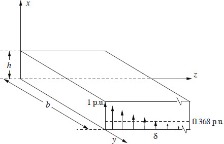
Figure 4.1 Penetration of field inside a conductor.

The total ohmic power loss is given by

$P=\frac{1}{\sigma }{\displaystyle \underset{v}{\int }{J}_u^2\text{d}v=\frac{1}{\sigma }\left(\frac{J_{xp}^2}{2}{\text{cos}}^2\left(\omega t-\frac{\pi }{4}\right)\right)bh\delta }.$

(4.56)

The average value of power can be expressed as

$P_{avg}=\frac{bh\delta }{2\sigma }{J}_{xp}^{2}avg\left({\text{cos}}^2\left(\omega t-\frac{\pi }{4}\right)\right)=\frac{bh\delta }{2\sigma }{J}_{xp}^{2}avg\left(\frac{1}{2}\left\{1+\text{ cos }2\left(\omega t-\frac{\pi }{4}\right)\right\}\right).$

(4.57)

Since the average value of a cosine term over an integral number of periods is zero we have

$P_{avg}=\frac{\delta bh}{4\sigma }{J}_{xp}^2$

(4.58)

which is the same as Equation 4.53. Hence, the average power loss in a conductor may be computed by assuming that the total current is uniformly distributed in one skin depth. This is an important result which can be used while calculating eddy current losses in conductors by numerical methods. When a numerical method such as FEM is used for estimating stray losses in the tank of a transformer, it is important to have the element size less than the skin depth of the tank material as explained earlier. With the overall dimensions of the field domain in meters, it is difficult to have very small elements inside the tank thickness. Hence, it is convenient to use analytical results to simplify the numerical analysis. For example, Equation 4.58 is used in [3] for the estimation of tank losses by 3-D FEM analysis. The method assumes uniform current density in the skin depth allowing the use of relatively larger element sizes. The above-mentioned problem of modeling and analysis of small skin depths can also be handled by using the concept of surface impedance. The intrinsic impedance can be rewritten from Equation 4.46 as

$\eta =R+jX=\sqrt{\frac{j\omega \mu }{\sigma }}=1\angle {45}^{°}\sqrt{\frac{\omega \mu }{\sigma }}=\sqrt{\frac{\omega \mu }{2\sigma }}+j\sqrt{\frac{\omega \mu }{2\sigma }}.$

(4.59)

The real part of the impedance, called surface resistance, is given by

$R=\sqrt{\frac{\omega \mu }{2\sigma }}.$

(4.60)

After calculating the r.m.s. value of the tangential component of the magnetic field intensity (H_rms) at the surface of the tank or any other structural component in the transformer by either numerical or analytical methods, the specific loss per unit surface area can be calculated by the following expression [4],

$P=R{H}_{rms}^2=\sqrt{\frac{\omega \mu }{2\sigma }}{H}_{rms}^2.$

(4.61)

Thus, the total losses in the transformer tank can be determined by integrating the specific loss over its internal surface.

4.3    Eddy Current and Hysteresis Losses

All the analysis done previously assumed linear material (B-H) characteristics meaning that the permeability (μ) is constant. The material used for structural components in transformers is usually magnetic steel (mild steel), which is a ferromagnetic material having a much larger value of relative permeability (μ_r) as compared to that of free space (for which μ_r =1). The material has nonlinear B-H characteristics and the permeability itself is a function of H. Moreover, the characteristics also exhibit hysteresis. Equation 4.6 (B = μ H) has to be suitably modified to reflect the nonlinear characteristics and the hysteresis phenomenon.

The core properties are generally expressed in terms of its permeability and losses. In an alternative way, the properties can be described by a single quantity known as complex (or elliptic) permeability. With the help of this type of representation, it is possible to represent the core by a simple equivalent electric circuit and the core losses can be expressed as a function of frequency.

If B is assumed to be a sinusoidal quantity, H will be non-sinusoidal due to a typical shape of the hysteresis loop. In the complex permeability representation, the harmonics are neglected, and only the fundamental components of B and H are considered. The magnetic field intensity (H) and the current are in phase, whereas the flux density (B) and the voltage are in perfect quadrature relationship; the voltage V leads B or flux by 90 degrees according to Equation 1.1 which in the time-harmonic form becomes [5]:

$\widehat{B}=\left(\frac{-j}{N\omega A_c}\right)\widehat{V}.$

Here, $\widehat{B}$ and $\widehat{V}$ are phasors, and A_c is the cross-sectional area having magnetic path length l with N turns wound around it. In this discussion on complex permeability, caps are put on phasor quantities. We also know that

$\widehat{H}=\left(\frac{N}{l}\right)\widehat{I}$

$\therefore \widehat{\mu }=\frac{\widehat{B}}{\widehat{H}}=\left(\frac{-jl}{N^2\omega A_c}\right)\widehat{Z}.$

The above equation represents the complex permeability in terms of impedance. If $\widehat{Z}$ is purely reactive, $\widehat{\mu }$ turns into a real quantity representing a lossless case, but if $\widehat{Z}$ is a complex quantity, then $\widehat{\mu }$ has an imaginary component as well, representing the lossy nature of the material. $\widehat{B}$ lags $\widehat{H}$ by a hysteresis angle as shown in Figure 2.5 (b), with $\widehat{H}$ having only the fundamental component (in the phasor notation, all the quantities vary sinusoidally at one frequency). In other words, we have achieved linearization with the hysteresis losses accounted in an approximate but reasonable way. In this formulation, where harmonics introduced by saturation are ignored, a functional relationship between B and H is now realized in which the permeability is made independent of H resulting in a linear system [6].

Let B₀ and H₀ be the peak values of the corresponding phasors. The relationship between B₀ and H₀ can be expressed as

$\begin{array}{ccc}\mu =B_0/H_0=\sqrt{{({\mu }^{\prime })}^2+{({\mu }^{″})}^2}& \text{and}& \theta ={\text{tan}}^{-1}({\mu }^{″}/{\mu }^{\prime })\end{array}$

(4.62)

where μ′ and μ″ are the real and imaginary components of the complex permeability. Here, the complex permeability is represented as

$\widehat{\mu }=\mu e^{-j\theta }.$

(4.63)

For the sinusoidal magnetic field intensity, H₀sin ωt, the flux density phasor can be expressed as [6]

$\widehat{B}=H_0({\mu }^{\prime }\text{ sin }\omega t+{\mu }^{″}\text{ cos }\omega t).$

Using this equation, we obtain an elliptic B-H curve as shown in Figure 4.2. The equation of the ellipse in the Cartesian form is [6]

$B={\mu }^{\prime }H\pm {\mu }^{″}\sqrt{H_0^2-H^2}.$

(4.64)

When H = H₀, B = μ′H₀ the slope of the line joining the origin and the point Q on the ellipse is μ′. On the other hand, when H = 0, B = B_r = ±μ″H₀ the slope of the line joining the point P and the y axis intercept (B_r) is in fact μ″. Thus, the real and imaginary components of the complex permeability can be determined from the aforesaid properties, if the B-H loop the material under investigation is determined experimentally.

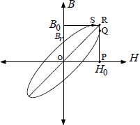
Figure 4.2 Elliptic hysteresis loop.

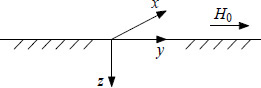
Figure 4.3 Infinite half space.

The area of the ellipse, (πµ″H₀²), gives the hysteresis loss per unit volume in one cycle. If there were no hysteresis losses, the phasors $\widehat{B}$ and $\widehat{H}$ would be in phase, and the permeability has only the real component and the ellipse collapses into a straight line.

Let us now find the expressions for the eddy and hysteresis losses for an infinite half-space shown in Figure 4.3. The infinite half-space is an extension of the geometry shown in Figure 4.1 in the sense that the region of the material under consideration extends from −∞ to +∞ in the x and y directions, and from 0 to ∞ in the z direction. Similar to Section 4.1, we assume that E and H vectors have components in only the x and y directions respectively, and that they are a function of z only. The diffusion Equation 4.15 can be rewritten for this case in terms of the complex permeability as

$\frac{d^2{H}_y}{d{z}^2}=j\omega (\mu e^{-j\theta })\sigma H_y.$

A solution satisfying boundary conditions,

$H_y=H_0\text{at}z=0\text{and}{H}_y=0\text{at}z=\infty$

is given by

$H_y=H_0{e}^{-kz}$

(4.65)

where the constant k is

$k=\sqrt{j\omega \sigma \mu e^{-j\theta }}=(1+j)\sqrt{\frac{\omega \mu \sigma }{2}}{e}^{\raisebox{1ex}{$-j\theta $}\!\left/ \!\raisebox{-1ex}{$2$}\right.}=\frac{\alpha +j\beta }{\delta }$

(4.66)

and

$\begin{array}{ccc}\alpha =\cos (\theta /2)+\sin (\theta /2)& \text{and}& \beta =\cos (\theta /2)-\sin (\theta /2)\end{array}.$

(4.67)

$\therefore H_y=H_0{e}^{\raisebox{1ex}{$-(\alpha +j\beta )z$}\!\left/ \!\raisebox{-1ex}{$\delta $}\right.}.$

(4.68)

Using Equation 4.8 and the fact that H_x = H_z = 0 we have

$J_x=-\frac{d}{dz}(H_y)=H_0\frac{\alpha +j\beta }{\delta }{e}^{\raisebox{1ex}{$-(\alpha +j\beta )z$}\!\left/ \!\raisebox{-1ex}{$\delta $}\right.}.$

(4.69)

The time average density of the eddy and hysteresis losses is determined by computing the real part of the complex Poynting vector evaluated at the surface [1],

$P_{e+h}=\frac{1}{2}\mathrm{Re}{[E\times H^{*}]}_{z=0}.$

(4.70)

Now,

$E={\left(\raisebox{1ex}{$J_x$}\!\left/ \!\raisebox{-1ex}{$\sigma $}\right.\right)}_{z=0}{a}_x=\frac{H_0}{\sigma \delta }(\alpha +j\beta )a_x$

(4.71)

and

$H=H_0{a}_y$

(4.72)

$\therefore P_{e+h}=\frac{1}{2}\mathrm{Re}\left[\frac{H_0}{\sigma \delta }(\alpha +j\beta )H_0{a}_z\right]=\frac{1}{2}\left[\frac{H_0^2}{\sigma \delta }\right]\alpha .$

(4.73)

In the absence of hysteresis (θ = 0), α = β = 1 according to Equation 4.67. Hence, the eddy loss per unit surface area is given by

$P_e=\frac{1}{2}\left[\frac{H_0^2}{\sigma \delta }\right].$

(4.74)

Substituting the expression for the skin depth from Equation 4.38 and using the r.m.s. value of the magnetic field intensity (H_rms) at the surface we obtain

$P_e=\frac{1}{2}\left[\frac{2H_{rms}^2}{\sigma }\right]\sqrt{\frac{\omega \mu \sigma }{2}}=\sqrt{\frac{\omega \mu }{2\sigma }}{H}_{rms}^2$

(4.75)

which is the same as Equation 4.61, as it should be in the absence of hysteresis (for linear B-H characteristics).

4.4    Effect of Saturation

In a transformer, the structural components (mostly made from a magnetic steel material) are subjected to a leakage field and/or a high current field. The incident field is predominantly concentrated in the skin depth near the surface. Hence, the structural components may be in a state of saturation depending upon the magnitude of the incident field. The eddy current losses predicted by the calculations based on a constant value of the relative permeability are usually smaller than experimental values. Thus, although the magnetic saturation is part and parcel of the hysteresis phenomenon, it is considerably more important in its effect on the eddy current losses. The step function magnetization curve, as shown in Figure 4.4 (a), is the simplest way of taking the saturation into account for an analytical solution of eddy current problems. It can be expressed by the equation,

$B=\left(s\text{ign}\text{of}H\right)B_s$

(4.76)

where B_s is the saturation flux density. The magnetic field intensity H at the surface is sinusoidally varying with time (= H₀ sin ωt). The extreme depth to which the field penetrates and beyond which there is no field is called the depth of penetration δ_s. This depth of penetration has a different connotation compared to that in the linear case discussed earlier. In this case, the depth of penetration is simply the maximum depth the field will penetrate at the end of each half period. A plate having thickness much larger than its depth of penetration is considered a thick one and it can be represented as an infinite half space; the corresponding depth of penetration is given by [1, 7, 8]

${\delta }_s=\sqrt{\frac{2H_0}{\omega \sigma B_s}}.$

(4.77)

It can be observed that for this nonlinear case with step magnetization characteristics, the linear permeability in Equation 4.38 is replaced by the ratio B_s/H₀. Further, the expression for the average power per unit area can be derived as

$P_e=\frac{8}{3\pi }\frac{H_0^2}{\sigma {\delta }_s}=1.7\frac{H_0^2}{2\sigma {\delta }_s}.$

(4.78)

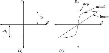
Figure 4.4 Step-magnetization.

Comparing this with Equation 4.74, it can be noted that if we put μ = B_s/H₀, δ_s will be equal to δ and in that case the loss in the saturated material is 70% higher than the loss calculated with linearly approximated B-H characteristics. Practically, the actual B-H curve is between the linear and step characteristics, as shown in Figure 4.4 (b). In [7], it is pointed out that as we penetrate inside the material, each succeeding inner layer is magnetized by a progressively smaller number of exciting ampere-turns because of the shielding effect of the eddy currents in the region between the outermost surface and the layer under consideration. In step magnetization characteristics, the flux density has the same magnitude irrespective of the magnitude of mmf. Due to this departure of the step curve response from the actual response, the value of B_s is replaced by 0.75 × B_s. From Equations 4.77 and 4.78, it is clear that $P_e\propto \sqrt{B_s}$, and hence the constant 1.7 in Equation 4.78 reduces to $1.7\times \sqrt{0.75}$, i.e., 1.47. As per Rosenberg’s theory, the constant is 1.33 [7]. Hence, in the simplified analytical formulations, linear characteristics are assumed after taking into account the nonlinearity by a linearization coefficient which is in the range of 1.3 to 1.5. For example, a value of 1.4 is used for the coefficient in [9] for the calculation of losses in the tank and the other structural components in transformers.

After having discussed the fundamentals of eddy currents, we will now analyze eddy current and circulating current losses in windings in the following sections. Analysis of stray losses in structural components, viz. the tank, frames, flitch plates, high current terminations, etc., is covered in Chapter 5.

4.5    Eddy Losses in Transformer Windings

4.5.1    Expression for the eddy loss

Theory of eddy currents explained in the previous sections will be useful while deriving the expression for the eddy loss occurring in windings. The losses in a transformer winding due to an alternating current are more than that due to a direct current of the same effective (r.m.s.) value. There are two different approaches for analyzing this increase in losses. In the first approach, we assume that the load current in the winding is uniformly distributed in the conductor cross section (similar to the direct current) and, in addition to the load current, there exist eddy currents which produce extra losses. Alternatively, one can calculate losses due to the combined action of the load current and the eddy currents. The former method is more suitable for the estimation of the eddy loss in windings, in which the eddy loss due to the leakage field (produced by the load current) is calculated separately and then added to the DC I² R loss. The latter method is preferred for calculating circulating current losses, in which the resultant current in each conductor is calculated first, followed by the calculation of losses (which give the total of the DC I² R loss and the circulating current loss). We will first analyze the eddy losses in windings in this section; the circulating current losses are discussed in the next section.

Consider a winding conductor, as shown in Figure 4.5, which is placed in an alternating magnetic field along the y direction having the peak amplitude of H₀. The conductor can be assumed to be infinitely long in the x direction. The current density J_x and the magnetic field intensity H_y are assumed as functions of z only. Rewriting the (diffusion) Equation 4.15 for the sinusoidal variation of the field quantity and noting that the winding conductor, either copper or aluminum, has constant permeability (linear B-H characteristics),

$\frac{d^2{H}_y}{d{z}^2}=j\omega \mu \sigma H_y.$

(4.79)

A solution satisfying this equation is

$H_y=C_1{e}^{\gamma z}+C_2{e}^{-\gamma z}$

(4.80)

where γ is defined by Equation 4.32. In comparison with Equation 4.65, Equation 4.80 has two terms representing waves traveling in both +z and −z directions (which is consistent with Figure 4.5). The incident fields on both the surfaces, having the peak amplitude of H₀, penetrate inside the conductor along the z axis in opposite directions. For the present case, the boundary conditions are

$H_y=H_0\text{at}z=+b\text{and}{H}_y=H_0\text{at}z=-b.$

(4.81)

Using these boundary conditions, we can obtain the expression for the constants as

$C_1=C_2=\frac{H_0{e}^{\gamma b}-H_0{e}^{-\gamma b}}{e^{2\gamma b}-e^{-2\gamma b}}=\frac{H_0}{e^{\gamma b}+e^{-\gamma b}}.$

(4.82)

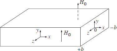
Figure 4.5 Estimation of eddy loss in a winding conductor.

Putting these values of the constants in Equation 4.80 we obtain

$H_y=\frac{H_0(e^{\gamma z}+e^{-\gamma z})}{e^{\gamma b}+e^{-\gamma b}}=H_0\frac{\cosh \gamma z}{\cosh \gamma b}.$

(4.83)

Using Equation 4.8 and the fact that H_x = H_z = 0, the current density is

$J_x=-\frac{d{H}_y}{dz}=-\gamma H_0\frac{\sinh \gamma z}{\cosh \gamma b}.$

(4.84)

The loss produced per unit surface area (of the x-y plane) of the conductor in terms of the peak value of the current density (|J_x|) is given by

$P_e=\frac{1}{2\sigma }\underset{-b}{\overset{+b}{{\displaystyle \int }}}|J_x{|}^{2}dz.$

(4.85)

Now, using Equation 4.39 we obtain

$\begin{array}{l}\left|J_x\right|=\left|-\gamma H_0\frac{\sinh \gamma z}{\cosh \gamma b}\right|=H_0\left|-\frac{1+j}{\delta }\frac{\sinh (1+j)z/\delta }{\cosh (1+j)b/\delta }\right|\\ =H_0\left|-\frac{1+j}{\delta }\times \frac{\sinh (z/\delta )\cos (z/\delta )+j\cosh (z/\delta )\sin (z/\delta )}{\cosh (b/\delta )\cos (b/\delta )+j\sinh (b/\delta )\sin (b/\delta )}\right|\\ =\frac{\sqrt{2}{H}_0}{\delta }{\left[\frac{{(\sinh (z/\delta )\cos (z/\delta ))}^2+{(\cosh (z/\delta )\sin (z/\delta ))}^2}{{(\cosh (b/\delta )\cos (b/\delta ))}^2+{(\sinh (b/\delta )\sin (b/\delta ))}^2}\right]}^{\raisebox{1ex}{$1$}\!\left/ \!\raisebox{-1ex}{$2$}\right.}\\ =\frac{\sqrt{2}{H}_0}{\delta }{\left[\frac{{(e^{z/\delta }-e^{-z/\delta })}^2{\cos }^2\left(z/\delta \right)+{(e^{z/\delta }+e^{-z/\delta })}^2{\sin }^2\left(z/\delta \right)}{{(e^{b/\delta }-e^{-b/\delta })}^2{\cos }^2\left(b/\delta \right)+{(e^{b/\delta }-e^{-b/\delta })}^2{\sin }^2\left(b/\delta \right)}\right]}^{\raisebox{1ex}{$1$}\!\left/ \!\raisebox{-1ex}{$2$}\right.}\\ =\frac{\sqrt{2}{H}_0}{\delta }{\left[\frac{(e^{2z/\delta }-e^{-2z/\delta })-2\left({\cos }^2\left(z/\delta \right)-{\sin }^2\left(z/\delta \right)\right)}{(e^{2b/\delta }-e^{-2b/\delta })+2\left({\cos }^2\left(b/\delta \right)-{\sin }^2\left(b/\delta \right)\right)}\right]}^{\raisebox{1ex}{$1$}\!\left/ \!\raisebox{-1ex}{$2$}\right.}\\ =\frac{\sqrt{2}{H}_0}{\delta }{\left[\frac{\cosh (2z/\delta )-\cos (2z/\delta )}{\cosh (2b/\delta )+\cos (2b/\delta )}\right]}^{\raisebox{1ex}{$1$}\!\left/ \!\raisebox{-1ex}{$2$}\right.}.\end{array}$

(4.86)

Substituting this magnitude of the current density in Equation 4.85 we have

$P_e=\frac{1}{2\sigma }\frac{2H_0^2}{{\delta }^2}{\displaystyle \underset{-b}{\overset{+b}{\int }}\frac{\cosh (2z/\delta )-\cos (2z/\delta )}{\cosh (2b/\delta )+\cos (2b/\delta )}dz}.$

(4.87)

$\therefore P_e=\frac{H_0^2}{\sigma \delta }\left[\frac{\sinh (2b/\delta )-\sin (2b/\delta )}{\cosh (2b/\delta )+\cos (2b/\delta )}\right]$

(4.88)

or

$P_e=\frac{H_0^2}{\sigma \delta }\left[\frac{e^{\xi }-e^{-\xi }-2\sin \xi }{e^{\xi }+e^{-\xi }+2\cos \xi }\right]$

(4.89)

where ξ = 2b/δ.

When 2b ≫ δ, i.e., ξ ≫ 1, Equation 4.89 can be simplified to

$P_e\approx \frac{H_0^2}{\sigma \delta }.$

(4.90)

Equation 4.90 gives the expression for the eddy loss per unit surface area of a conductor with its dimension, perpendicular to the applied field, much greater than the depth of penetration. Such a case, with the field applied on both surfaces of the conductor, is equivalent to two infinite half spaces. Therefore, the total eddy loss given by Equation 4.90 is two times that of the infinite half space analyzed earlier (Equation 4.74). For such thick conductors/plates (windings made of copper bars, structural components made from a magnetic steel material having sufficiently large thickness, etc.), the resultant current distribution is greatly influenced and limited by the effect of its own field and the currents are said to be inductance-limited [1] (currents are confined to the surface layers).

Now, let us analyze the case when the conductor thickness is much smaller than its depth of penetration, which is usually the case for rectangular paper insulated conductors used in transformers. For 2b ≪ δ, i.e., ξ ≪ 1, Equation 4.89 can be simplified to

$\begin{array}{ll}{P}_e\hfill & =\frac{H_0^2}{\sigma \delta }\left[\frac{\left(1+\xi +\frac{{\xi }^2}{2!}+\frac{{\xi }^3}{3!}\cdots \right)-\left(1-\xi +\frac{{\xi }^2}{2!}-\frac{{\xi }^3}{3!}\cdots \right)-2\left(\xi -\frac{{\xi }^3}{3!}\cdots \right)}{\left(1+\xi +\frac{{\xi }^2}{2!}+\frac{{\xi }^3}{3!}\cdots \right)+\left(1-\xi +\frac{{\xi }^2}{2!}-\frac{{\xi }^3}{3!}\cdots \right)+2\left(1-\frac{{\xi }^2}{2!}\cdots \right)}\right]\hfill \\ \hfill & =\frac{H_0^2}{\sigma \delta }\left[\frac{\left(4\frac{{\xi }^3}{3!}+\cdots \right)}{4+4\frac{{\xi }^4}{4!}+\cdots }\right]\hfill \end{array}$

(4.91)

Neglecting the higher order terms and substituting the expression of δ from Equation 4.38 we have

$P_e=\frac{H_0^2}{\sigma \delta }\frac{{\xi }^3}{6}=\frac{H_0^2}{\sigma \delta }\frac{8b^3}{6{\delta }^3}=\frac{H_0^2}{\sigma }\frac{8b^3{\omega }^2{\mu }^2{\sigma }^2}{24}=\frac{1}{3}{(\mu H_0)}^2\sigma {\omega }^2{b}^3.$

(4.92)

Now, if the thickness of the winding conductor is t, then substituting b = t / 2 in Equation 4.92 we obtain

$P_e=\frac{1}{3}{B}_0^2\sigma {\omega }^2{\left(\frac{t}{2}\right)}^3=\frac{{\omega }^2{B}_0^2{t}^3\sigma }{24}.$

(4.93)

It is more convenient to find an expression for the mean eddy loss per unit volume (since the volume of the conductor in the winding is usually known). Hence, dividing by t and finally substituting ρ (resistivity) as 1/σ, we obtain the expression for the eddy loss in the winding conductor per unit volume as

$P_E=\frac{{\omega }^2{B}_0^2{t}^2}{24\rho }.$

(4.94)

In the case of thin conductors, the eddy currents are said to be resistance-limited since they are restricted by lack of space or high resistivity [1]. In other words, since the field of the eddy currents is negligible for thin conductors, the behavior is dominated by resistive effects. Equation 4.94 matches exactly with that derived in [10] by ignoring the magnetic field produced by the eddy currents. These currents are 90° out of phase with the uniformly distributed load current flowing in the conductor, which produces the leakage field and is also responsible for the DC I²R loss in windings. The eddy currents are shown to be lagging by 90° with respect to the load (source) current for a thin circular conductor in a later part of this section. The total current flowing in the conductor can be visualized to be a vector sum of the eddy current (Ieddy) and load current (I_load) components, having the magnitude of $\sqrt{{(I_{eddy})}^2+{(I_{load})}^2}$, because these two current components are 90° out of phase in a thin conductor. This is a very important and convenient result because it means that the I² R losses due to the load current and the induced eddy currents can be calculated separately and then added later for thin conductors.

Equation 4.94 is a very well-known and useful formula for the calculation of the eddy loss in windings. If we assume that the leakage field in windings is in the axial direction only, we can calculate the mean value of the eddy loss in the whole winding by using the theory in Section 3.1.1. The axial leakage field for an inner winding (having radial depth R and height H_W) varies linearly from its inside diameter to outside diameter as shown in Figure 4.6. The thickness of the conductor, the dimension perpendicular to the axial field, is usually small. Hence, the same value of flux density (B₀) can be assumed along its two vertical surfaces. The position of the conductor changes along the radial depth as the turns are wound. Hence, in order to calculate the mean value of the eddy loss of the whole winding, we have to first calculate the mean value of $B_0^2$. The r.m.s. value of the ampere turns change linearly from 0 at the inside diameter (ID) to NI at the outside diameter (OD). The peak value of the flux density at a distance x from the inside diameter is

$B_x=\frac{\sqrt{2}{\mu }_0}{H_W}\left[\left(\frac{x}{R}\right)NI\right].$

(4.95)

The mean flux density value, which gives the same overall loss, is given by

${(B_0^2)}_{mean}=\frac{1}{R}{\displaystyle \underset{0}{\overset{R}{\int }}{\left[\frac{\sqrt{2}{\mu }_{0}NI}{H_W}\right]}^2\frac{x^2}{R^2}dx.}$

(4.96)

Simplifying we obtain

${(B_0^2)}_{mean}=\frac{(B_{gp}^2)}{3}$

(4.97)

where B_gp is the peak value of the flux density in the LV-HV gap,

$B_{gp}=\frac{\sqrt{2}{\mu }_{0}NI}{H_W}.$

(4.98)

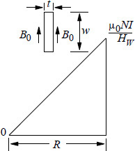
Figure 4.6 Leakage flux density distribution in a winding.

Hence, using Equations 4.97 and 4.94, the mean eddy loss per unit volume of the winding due to the axial leakage field is expressed as

${(P_E)}_{mean}=\frac{{\omega }^2{t}^2}{24\rho }\frac{B_{gp}^2}{3}.$

(4.99)

If we are interested in determining the mean value of the eddy loss in a section of a winding in which ampere-turns are changing from a(NI) at ID to b(NI) at OD, where NI are rated r.m.s. ampere-turns, the expression for the mean value of $B_0^2$ can be determined by using a procedure similar to that given in Section 3.1.1,

${(B_0^2)}_{mean}=\frac{(B_{gp}^2)}{3}[a^2+ab+b^2]$

(4.100)

and the mean eddy loss per unit volume in the section is

${(P_E)}_{mean}=\frac{{\omega }^2{t}^2}{24\rho }\frac{(B_{gp}^2)}{3}[a^2+ab+b^2].$

(4.101)

Equation 4.101 tells us that for a winding consisting of a number of layers, the mean eddy loss of the layer adjacent to the LV-HV gap is higher than that of the other layers. For example, in the case of a 2-layer winding,

$\begin{array}{cc}{(B_0^2)}_{mean}=\frac{(B_{gp}^2)}{3}\left[{\left(\frac{1}{2}\right)}^2+\frac{1}{2}\times 1+1^2\right]=1.75\frac{(B_{gp}^2)}{3}& \left(\text{for}\text{the}\text{second}\text{layer}\right)\end{array}$

indicating that the mean eddy loss in the second layer close to the gap is 1.75 times the mean eddy loss for the entire winding. Similarly, for a 4-layer winding,

$\begin{array}{cc}{(B_0^2)}_{mean}=\frac{(B_{gp}^2)}{3}\left[{\left(\frac{3}{4}\right)}^2+\frac{3}{4}\times 1+1^2\right]=2.31\frac{(B_{gp}^2)}{3}& \left(\text{for}\text{the}\text{fourth}\text{layer}\right)\end{array}$

giving the mean eddy loss in the 4^th layer as 2.31 times the mean eddy loss for the entire winding. Hence, it is always advisable to calculate the total loss (I² R + eddy) in each layer separately and estimate its temperature rise. Such a calculation procedure helps designers in taking countermeasures to eliminate high temperature rise problems in windings. Also, the temperatures measured by fiber-optic sensors (if installed) will be closer to the calculated values when this calculation procedure is adopted.

Eddy loss calculated by Equation 4.99 is approximate since it assumes that the leakage field is entirely in the axial direction. As seen in Chapter 3, there exists a radial component of the leakage field at winding ends and in winding zones where ampere-turns per unit height are different for the LV and HV windings. For small distribution transformers, the error introduced by neglecting the radial field may not be appreciable, and Equation 4.99 is generally used with some empirical correction factor applied to the total calculated stray loss value. Analytical/numerical methods, described in Chapter 3, need to be used for the correct estimation of the radial field. The amount of effort required for obtaining the accurate eddy loss value might not be justified for small-distribution transformers. For medium- and large-power transformers, however, the eddy loss due to the radial field has to be estimated and the same can be determined by using Equation 4.94, for which the dimension of the conductor perpendicular to the radial field is its width w. Hence, the eddy losses per unit volume due to the axial (B_y) and radial (B_x) components of the leakage field are

${(P_E)}_{axial}=\frac{{\omega }^2{B}_y^2{t}^2}{24\rho }$

(4.102)

${(P_E)}_{radial}=\frac{{\omega }^2{B}_x^2{w}^2}{24\rho }.$

(4.103)

Thus, the leakage field incident on a winding conductor (see Figure 4.7) is resolved into two components, viz. B_y and B_x, and losses due to these two components are calculated separately by Equations 4.102 and 4.103, and then added. This is permitted because the eddy currents associated with these two perpendicular components do not overlap (since the angle between them is 90°).

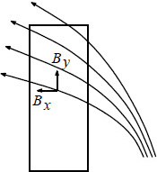
Figure 4.7 Winding conductor in a leakage field.

We have assumed that the conductor dimension is very much less than the depth of penetration while deriving Equation 4.94. This is particularly true in the case of the loss due to the axial field. The conductor thickness used in transformers mostly falls in the range of 2 to 3.5 mm and is considerably less than the depth of penetration of copper and aluminum, which is 10.3 mm and 13.2 mm, respectively, at 50 Hz. The conductor width is usually closer to the depth of penetration. If the conductor width is equal to the depth of penetration (w = 2b = δ), Equation 4.89 becomes

$\begin{array}{cc}{(P_e)}_{2b=\delta }=\frac{H_0^2}{\sigma \delta }\left[\frac{e^1-e^{-1}-2\sin 1}{e^1+e^{-1}+2\cos 1}\right]=\frac{1}{6.24}\frac{H_0^2}{\sigma \delta }& :fromtheexactequation.\end{array}$

Comparing this value with that given by Equation 4.92,

$\begin{array}{cc}{(P_e)}_{2b=\delta }=\frac{H_0^2}{\sigma \delta }\frac{{\xi }^3}{6}=\frac{1}{6}\frac{H_0^2}{\sigma \delta }& :fromtheapproximateequation,\end{array}$

an error of just 4% is obtained, which is acceptable. Hence, it can be concluded that the eddy loss due to the radial field can also be calculated with reasonable accuracy from Equation 4.103 for the conductor width comparable to the depth of penetration.

For thin circular conductors of radius of R, if the ratio R / δ is small, we can neglect the magnetic field of eddy currents. If the total current in the conductor is I cos ω t, the uniform current density is given by

$J_0=\frac{I}{\pi R^2}\cos \omega t$

(4.104)

and the eddy current density at any radius r inside the conductor is [8]

$J_e=\frac{I}{2\pi {\delta }^2}\left[\frac{1}{2}-\frac{r^2}{R^2}\right]\sin \omega t.$

(4.105)

Thus, it can be observed from Equations 4.104 and 4.105 that for thin conductors (exhibiting resistance-limited behavior), the eddy currents lag the exciting current that produces the field responsible for them by 90°. Contrary to this, for thick conductors (with the thickness or radius much larger than the depth of penetration), the eddy currents lag the exciting current by 180° (this is an inductance-limited behavior in which the currents are confined to the surface layers).

The power loss per unit length of the thin circular conductor can be determined by using Equations 4.104 and 4.105 as (J₀ and J_e are 90° apart, square of their sum is equal to the sum of their squares)

$P_1={\displaystyle \underset{0}{\overset{R}{\int }}\left[\frac{|J_0{|}^2+|J_e{|}^2}{2\sigma }\right]}2\pi rdr=\frac{I^2}{2\pi R^2\sigma }+\frac{I^2{R}^2}{96\pi \sigma {\delta }^4}.$

(4.106)

The power loss per unit length due to the exciting current alone is

$P_2={\left(\frac{I}{\sqrt{2}}\right)}^2\times \frac{1}{\sigma }\times \frac{1}{\pi R^2}.$

(4.107)

Therefore, the ratio of the effective AC resistance to the DC resistance of the thin circular conductor can be deduced from Equations 4.106 and 4.107 as

$\begin{array}{cc}\frac{R_{AC}}{R_{DC}}=\frac{P_1}{P_2}=1+\frac{1}{48}{\left(\frac{R}{\delta }\right)}^4& \cdots forthincircularconductors\end{array}.$

(4.108)

For thick circular conductors (R ≫ δ), the effective resistance is that of an annular ring of diameter 2R and thickness δ, since all the current can be assumed to be concentrated in one depth of penetration as discussed in Section 4.2. Hence, the effective AC resistance per unit length is

$R_{AC}=1/(2\pi R\delta \sigma )$

(4.109)

and

$\begin{array}{cc}\frac{R_{AC}}{R_{DC}}=\frac{R}{2\delta }& \cdots forthinkcircularconductors\end{array}.$

(4.110)

4.5.2    Methods of estimation

As said earlier, the axial and radial components of a leakage field distribution can be estimated by analytical or numerical methods. Accurate estimation of the eddy loss due to the radial component by means of empirical formulae is not possible. Analytical methods [11, 12] and 2-D FEM [13, 14] can be used to calculate the eddy loss due to axial and radial leakage fields. It is assumed that the eddy currents do not have influence on the leakage field (i.e., a case of thin conductors). The FEM analysis is commonly used for the eddy loss calculations. The winding is divided into many sections. For each section the corresponding ampere-turn density is defined. The value of conductivity is not defined for these sections. The values of B_y and B_x for each conductor can be obtained from the FEM solution, and then the axial and radial components of the eddy loss are calculated for each conductor by using Equations 4.102 and 4.103, respectively. The B_y and B_x values are assumed to be constant over the conductor cross-section and are taken as equal to the corresponding values at its center. In cylindrical coordinates, B_y and B_x components are replaced by B_z and B_r components, respectively. The total eddy loss for each winding is calculated by integrating the loss components of all its conductors.

Sometimes a quick but reasonably accurate estimate of the eddy loss is required. At the tender design stage, an optimization program may have to work out hundreds of options to arrive at an optimum design. In such cases, expressions for the eddy loss in windings for standard configurations can be determined using a multiple regression method in conjunction with an Orthogonal Array Design of Experiments technique [15]. However, due to rapid developments in computing facilities, it is now possible to integrate more accurate analytical or 2-D numerical methods into design optimization programs.

For cylindrical windings in core-type transformers, two-dimensional methods give sufficiently accurate eddy loss values. For getting the most accurate results, three-dimensional magnetic field calculations have to be performed [16, 17, 18]. Once a three-dimensional field solution is obtained, the three components of the flux density (B_x, B_y and B_z) are resolved into two components, viz. the axial and radial components; this approach enables the use of Equations 4.102 and 4.103 for the eddy loss evaluation.

For distribution transformers whose LV winding is made using a thick rectangular bar conductor, each and every turn of the winding has to be modeled (with the value of conductivity defined) in the FEM analysis. This is because the thickness of the bar conductor is usually comparable to or sometimes more than the depth of penetration, and its width is usually more than 5 times the depth of penetration. With such a conductor having large dimensions, a significant modification of the leakage field occurs due to the eddy currents, which cannot be neglected in the calculations.

4.5.3    Optimization of losses and elimination of winding hot spots

While designing a winding, if the designer increases conductor dimensions to reduce the DC resistance (I² R) loss, the eddy loss increases. Hence, optimization of the sum of the I² R and eddy losses should be done.

The knowledge of flux density distribution within a winding helps in choosing proper dimensions of its conductor. This is particularly important for windings having tappings within their body; high values of radial field in the tap zone can cause excessive loss and temperature rise problems. For minimization of radial flux, balancing of ampere-turns per unit height of the LV and HV windings should be done (for various sections along their height) at the average tap position. The winding with taps can be designed with different conductor dimensions in the tap zone to minimize the risk of hot spots. Guidelines are given in [19] for choosing the conductor width for eliminating hot spots in windings. For 50 Hz frequency, the maximum width that can be used is usually in the range of 12 to 14 mm, whereas for 60 Hz it is of the order of 10 to 12 mm. This guideline is useful in the absence of a detailed calculation of temperature rise distribution in the part of the winding where a hot spot is suspected. For calculating the temperature rise of a disk or a turn, its I² R loss and eddy loss should be added. An idle winding between the LV and HV windings links the high gap flux resulting in a substantial amount of eddy loss in it. Hence, its conductor dimensions should be properly decided.

In gapped core shunt reactors, there is considerable flux fringing between consecutive limb packets (separated by a non-magnetic gap), resulting in appreciable radial flux causing excessive losses in their winding if its distance from the core is small or if the conductor width is large.

One of the most logical ways of reducing the eddy loss of a winding is to subdivide winding conductors into a number of parallel conductors. If a conductor having thickness t is subdivided into two insulated parallel conductors, each of thickness t / 2, the eddy loss due to the axial leakage field reduces by a factor of 1/4 (according to Equation 4.102). However, there is a limitation imposed on the minimum value of thickness that can be used from the short-circuit withstand considerations. Also, if the width to thickness ratio of a rectangular conductor is more than about 6, there may be difficulty in winding it. The subdivision of the conductor also impairs the winding space factor in the radial direction. This is because each individual parallel conductor in a turn has to be insulated increasing the total insulation thickness in the direction. In order to improve the space factor, sometimes a bunch conductor is used in which usually two or three parallel conductors are bunched in a common paper covering. The advantage is that each conductor needs to be insulated with a lower paper insulation thickness because of the outermost common paper covering. A single bunch conductor is also easier to wind, since no crossovers are required at ID and OD of the winding. In contrast to this, for example in the case of two parallel conductors, the conductors are usually crossed over at ID and OD of each disk for the ease of winding. Three rectangular strip conductors and the corresponding bunch conductor are shown in Figure 4.8. For a strip conductor having radial thickness of 2 mm and paper covering of 0.5 mm, the total radial dimension of the three strip conductors is 9 mm, whereas for a bunch conductor having individual radial insulation of 0.175 mm and common outermost radial insulation of 0.325 mm, the total radial dimension is 7.7 mm (=3 × e (2+2 × 0.175)+2 × 0.325) giving 15% improvement in the space factor.

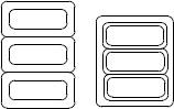
Figure 4.8 Strip and bunch conductor.

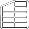
Figure 4.9 CTC conductor.

For a continuously transposed cable (CTC) conductor, in which a number of small rectangular conductors are transposed at regular intervals, it is possible to use much smaller thickness (as low as 1.2 mm) and width (as low as 3.8 mm), reducing the eddy loss considerably. Cost-benefit analysis has to be done to check the advantage gained by the reduction of losses vis-à-vis a higher cost of the CTC conductor. For a transformer specification with a high value of the load loss capitalization (dollars per kW of the load loss), the CTC conductor may give a lower total capitalized cost (i.e., the sum of material and loss costs) particularly in large transformers. The LV winding in large generator transformers is usually designed using a CTC conductor to minimize the eddy loss and improve productivity. A typical CTC conductor is shown in Figure 4.9.

One more way of reducing the eddy loss is by the use of a combination of two conductors with different widths along the winding height. At the winding ends, there may be an appreciable eddy loss due to the fact that the radial flux is incident perpendicularly on the wider conductor dimension (width). This loss can be decreased by reducing the conductor width for few disks at the ends using FEM-based calculations. The width of the conductor for the remaining middle portion, which has predominantly an axial field, is increased to have the same overall height, so that the I² R losses are maintained approximately constant. Such an arrangement can give reduction in the winding loss (I² R + eddy) by about 1 to 2% in large transformers.

In another method, end disks can have fewer turns per disk (one or two turns less compared to the remaining disks) in the HV winding having a large number of turns per disk. A conductor with higher thickness and lower width can be used for these disks so that I² R loss is kept approximately constant and the eddy loss is reduced. This scheme is useful when the increase in the axial eddy loss due to a higher thickness is smaller than the decrease in the radial eddy loss due to a lower width (which may be particularly true at the ends since a reduction in the axial field value is accompanied by an increased radial field).

In both these methods, ampere-turns of the HV and LV windings per unit height should be equal (for various sections along their height); otherwise there will be an extra radial flux and the corresponding losses, nullifying the advantages gained.

A combination of strip and CTC conductors can be used to minimize the winding losses. A CTC conductor is used for a few top and bottom disks reducing the eddy loss, whereas the remaining disks are wound using a strip conductor. This technique requires establishment of a proper method for making the joint between the two types of conductors.

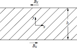
Figure 4.10 Foil winding analysis.

4.5.4    Eddy loss in foil windings

In small transformers, foil windings (made up of thin sheets of copper or aluminum) are popular because of the simplicity obtained in winding operations. A metal foil and an insulation layer can be wound simultaneously on a special machine and the whole process can be mechanized. In these windings, the eddy loss due to the axial leakage field is insignificant because of the thinness of the foil. On the contrary, radial field at the ends of the winding results in a substantial amount of the (radial) eddy loss.

The eddy loss in a foil winding can be evaluated by analytical or numerical methods. The eddy current density has been obtained as a solution of an integral equation of Fredholm type for a two winding transformer in [20]. For specific transformer dimensions given in the paper, the coefficient for the additional loss is 1.046; i.e., the eddy loss is 4.6% of the DC I² R loss. In another approach [21], a boundary-value field problem formulated in terms of the magnetic vector potential in cylindrical coordinates is solved using modified Bessel and Struve functions. For symmetrically placed LV (foil) and HV windings, the additional loss factor reported in the paper is 5.8%. For an asymmetrical arrangement of windings, this loss would increase.

In [22], the foil winding is assumed a vertical section of an infinitely wide and deep conducting plate which is assumed symmetrically penetrated on both sides by plane electromagnetic waves. The geometry is given in Figure 4.10, where h is the height of the foil winding and B_x denotes the value of the flux density at the winding ends. The induced eddy current density (with the vertical dimensions specified with respect to the middle of the winding height) is [22]

$J_e=\frac{B_x}{{\mu }_0\delta }{e}^{\left[\raisebox{1ex}{$-\left(\frac{h}{2}-y\right)$}\!\left/ \!\raisebox{-1ex}{$\delta $}\right.\right]}\left[\cos \left(\frac{\pi }{4}-\frac{\frac{h}{2}-y}{\delta }\right)+j\sin \left(\frac{\pi }{4}-\frac{\frac{h}{2}-y}{\delta }\right)\right].$

(4.111)

The eddy loss in terms of the peak value of the current density is given as

$P_e=\frac{1}{2\sigma }{\displaystyle \underset{v}{\int }|J_e{|}^{2}dv.}$

(4.112)

It is clear from Equations 4.111 and 4.112 that

$P_e\propto |J_e{|}^2\propto e^{\left[-2\left(\frac{h}{2}-y\right)/\delta \right]}.$

(4.113)

Hence, the eddy loss is maximum at y = h / 2 (at the two winding ends) since at this height the exponential term has the maximum value of 1,

$e^{\left[-2\left(\frac{h}{2}-y\right)/\delta \right]}=1$

whereas its value is just 0.0067 at y = (h / 2) − 2.5δ, which means that more than 99% of the induced eddy loss occurs in just 2.5δ depth from the winding ends. For an aluminum foil winding, whose skin depth is 13.2 mm at 50 Hz, almost all the eddy loss is concentrated in 33 mm from the winding ends. The foil winding eddy current density distribution calculated by Equation 4.111 for a typical transformer is shown in Figure 4.11.

Thus, the current density at the ends can be about 1.5 to 2 times the uniform current density, resulting in local heating of 2.25 to 4 times that in the middle portion of the winding. Hence, the temperature rise at the foil winding ends should be carefully assessed.

Usually, there is no temperature rise problem in foil windings since the thermal conductivity of aluminum/copper is quite good, and the winding edges are generally well exposed to the cooling medium. If a transformer with a foil winding is supplying a power electronic load, there is an increase in the heating effect at the ends of the winding on account of harmonics [23].

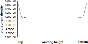
Figure 4.11 Eddy current distribution in a foil winding.

With the rapid development in computational facilities, numerical tools such as FEM can be easily applied to analyze the eddy loss distribution in foil windings without having to do any approximations as in analytical formulations. It is actually a three-dimensional problem; the loss in the foil winding calculated in the core-window cross section is lower than that calculated in the region outside the window. The radial flux at winding ends is usually more in the region outside the window, and hence the additional loss factor may be of the order of 10 to 15%. The position of the foil winding affects its eddy loss significantly. If it is the outer winding, the radial flux density at its ends reduces resulting in reduction of the eddy loss [24].

4.6    Circulating Current Loss in Transformer Windings

We have seen that the leakage field is responsible for extra losses in windings in addition to the DC I²R loss. If the windings have a single solid conductor then eddy currents flow causing the eddy loss, and no circulating current loss appears. In the windings with large current ratings, conductors have to be subdivided into a number of parallel conductors to reduce the eddy loss to an acceptable/optimum value. Without a proper transposition arrangement, the leakage flux linked by these parallel conductors is different, inducing different voltages in them. Since the conductors are paralleled at their ends, there will be net induced voltages in the loops formed by these conductors resulting in circulating currents. These circulating currents flow back and forth within the parallel conductors and thus do not flow outside the winding. The appearing value of the circulating current loss adds to the other stray loss components.

The circulating current loss depends very much on the physical locations of the conductors in the leakage field. This loss can be avoided if the locations of each conductor at various positions along the winding height are such that all the conductors link an equal amount of leakage flux. Such a winding is said to have an ideal transposition scheme in which each conductor occupies the position of every other conductor. This can be achieved by doing suitable transpositions between the parallel conductors. In the absence of transpositions, the advantage gained through the eddy loss reduction (by subdivision of conductors) will be lost due to the circulating current loss. Inaccurate or inadequate transpositions introduce circulating currents in windings, which can be calculated by either analytical or numerical methods.

4.6.1    Analytical methods

Analytical formulae are given in [25] to calculate the circulating current loss for various types of windings. In this formulation, the ampere-turn diagram is assumed to have a trapezoidal form. The leakage flux density (B) at the inside of the conductor and in the paper covering is calculated. Integrating this value of B over the thickness, the flux/cm is obtained. The voltage gradient is then calculated as the sum of the resistance drops of the load current and the stray currents (the eddy plus circulating currents), and the reactive drop induced by the flux. The circulating current component is calculated assuming that it is uniform in the whole cross section of the conductor. The effect of circulating currents on the leakage field has been neglected in this approximate method. Hence, it gives a higher value of the circulating current loss than that observed in practice.

It is shown in the paper that the circulating current loss for an untransposed layer winding is the same as the eddy loss in an equivalent one solid conductor. In other words, if a winding conductor having thickness t is split into two conductors each having thickness t/2, the circulating current loss for the untransposed case of these two conductors is the same as the eddy loss in the equivalent one conductor having thickness t. Hence, if a winding conductor is subdivided into parallel conductors which are untransposed, the total stray loss in the winding (eddy and circulating losses) will theoretically remain unchanged.

In order for each conductor to occupy the original position of every other conductor over an equal distance, various transposition schemes are used depending upon the type of winding and its conductor. Two such schemes are shown in Figure 4.12 for a layer winding with four parallel conductors. In both cases, each conductor occupies all four positions over an equal distance and hence all the conductors link the same value of leakage field (assuming that the field is entirely in the axial direction) resulting in no circulating currents.

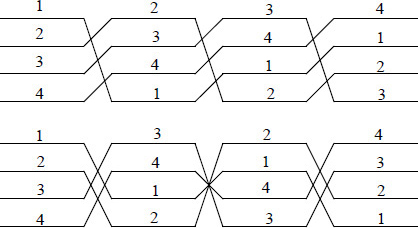
Figure 4.12 Transposition schemes in a layer winding.

Figure 4.13 Transposition scheme for 5 parallel conductors.

In general, for n parallel conductors one ideally needs n −1 transpositions equally spaced along the winding height. For example, in the case of 5 parallel conductors, there should be 4 transpositions as shown in Figure 4.13. At every transposition, the top conductor is brought to the bottom position. A thin rectangular copper strip of nearly the same cross-sectional area (as that of the conductor) can be used to join the two cut parts of the conductor by a brazing operation. Alternatively, the conductor can be brought to the bottom position without the cutting and brazing operations by providing a slanting support made from an insulation material.

There is one more scheme [26, p. 147 of 25] which can be used in small transformers in which only 3 transpositions are done in place of n −1 transpositions in order to reduce the manufacturing time. A typical scheme is shown in Figure 4.14 for 12 parallel conductors. In this scheme, parallel conductors are divided into four groups for the middle transposition, and hence the number of parallel conductors has to be a multiple of 4.

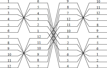
Figure 4.14 Transposition scheme for 12 parallel conductors.

This is not a perfect transposition scheme since none of the conductors is occupying the original position of every other conductor. But each conductor occupies 4 positions so that the average value of the field, linked by it, is not much different than that of the others when only the axial field is considered. The transposition scheme may be used with caution in small transformers when the radial field at ends and within the body of windings is insignificant.

In the discussion of paper [25], Rabins and Cogbill have given a very useful and quick method to check the correctness of any transposition scheme. According to this method, for each conductor a sum

$s={\displaystyle \sum \frac{N_p}{N}p(p-1)}$

is calculated where p is a particular position and N_p is the number of turns (out of total turns N) in position p. Let us apply the method to evaluate the transposition scheme given in Figure 4.14. Conductor 1 in Figure 4.14 occupies positions 1, 6, 9 and 10 for which s₁ = 0.25× (1× 0 + 6 × 5 + 9 × 8 +10 × 9) = 48. Similarly, the value of s for the remaining conductors can be determined. Here, it is assumed that the conductor occupies each of the 4 positions for 25% of the winding height. If this is not true or if a transposition is missed by one turn or one disk by mistake during manufacturing, the corresponding number of turns in each position should be taken. Closeness of s values for all the parallel conductors is a good indicator of the correctness of the transposition scheme. The average of the s values for all the conductors is calculated (s_avg). The circulating current (P_cc) loss is expressed in terms of the winding eddy loss (P_eddy) as

$P_{cc}=P_{eddy}\left(\frac{45}{5n^2-1}\right){\left(\frac{t+t_i}{t}\right)}^2\left[\frac{1}{n}{\displaystyle \sum }_1^n{(s_n-s_{avg})}^2\right]$

(4.114)

where t and t_i is the thickness of the conductors and the thickness of the insulation between adjacent conductors, respectively. For example, if the values of t and t_i are 2.3 mm and 0.5 mm, respectively, for the winding shown in Figure 4.14, P_cc = 0.0206 P_eddy, which is negligible. This indicates that the transposition scheme given in Figure 4.14, although not a perfect one, is sufficiently good to reduce the circulating current loss to a very low value. It should be noted that the calculation accounted for the axial leakage field only. Hence, the method may be used for small transformers only, when the radial field in them is low. The transposition scheme will not be effective if there is a significant radial field in any part of the winding. Also, at the middle transposition, the conductors have to be properly supported while they are being transposed, which otherwise may be vulnerable when subjected to short circuit forces.

Now, let us analyze continuous disk windings having a number of turns in the radial direction with each turn having two or more parallel conductors. Usually, the number of parallel conductors in a continuous disk winding is less than that in a layer winding. Hence, the problem of circulating currents is less ominous in continuous disk windings since the radial depth of each of the turns is smaller. A continuous disk winding, having N_d turns/disk and n parallel conductors per turn and crossovers between the conductors at the inside and outside diameters of every disk, is equivalent to a multi-layer winding having N_d layers with each layer having n parallel conductors transposed at its center (at the mid-height position).

A continuous disk winding with 8 parallel conductors and 3 turns per disk is shown in Figure 4.15. Kaul’s formula [25] for estimation of the circulating current loss for such a continuous winding with n parallel conductors is

$P_{cc}=2.4\times {10}^6\times \frac{1}{180}{(kR)}^4\left[1-\frac{5}{n^2}+\frac{4}{n^4}\right]\times \left(I^{2}RLoss\right)$

(4.115)

where

R = radial depth of the insulated turn = n (t + t_i)

$k=0.48\times {10}^{-4}\times \sqrt{\frac{h_c}{h_w}\frac{t}{(t+t_i)}\frac{f}{\rho }}$

(4.116)

ρ	= resistivity of the conductor material (copper or aluminum)
hc	= total length (height) of copper or aluminum in the axial direction
hw	= length (height) of the winding in the axial direction.

Ratios h_c / h_w and t/(t + t_i) define the space factors of the winding in the axial and radial directions, respectively. Let us calculate the circulating current loss for the winding shown in Figure 4.15 with the following parameters:

f = 50 Hz

t = 2.4 mm, t_i = 0.7 mm

h_c / h_w = 0.8

ρ = 0.0211 × 10⁻⁶ ohm-m (copper conductor).

∴ R = 8 × (2.4 + 0.7) ×10⁻³ = 0.0248 m

and

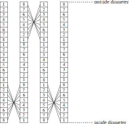
Figure 4.15 Continuous disk winding.

$k=0.48\times {10}^{-4}\times \sqrt{0.8\times \frac{2.4}{2.4+0.7}\times \frac{50}{0.0211\times {10}^{-6}}}=\mathrm{1.839.}$

The circulating current loss in the winding is

$\begin{array}{ll}{P}_{cc}\hfill & =2.4\times {10}^6\times \frac{1}{180}{(1.839\times 0.0248)}^4\left[1-\frac{5}{8^2}+\frac{4}{8^4}\right]\times \left(I^{2}RLoss\right)\hfill \\ \hfill & =0.053\times \left(I^{2}RLoss\right).\hfill \end{array}$

For I² R loss of 130 kW for this winding (for all three-phases), the total circulating current loss is about 6.9 kW, which is a significant value. This circulating current loss can be almost eliminated by doing the group transpositions at appropriate places similar to that for the layer winding shown in Figure 4.14.

It should be noted that in the analytical methods discussed so far, only the axial leakage field is considered and the effect of the radial leakage field is neglected. Due to this assumption the calculation is easy, and the extra loss on account of circulating currents can be determined quickly while the transformer design is in progress. Although these methods may not give the accurate loss value, designers can use them to check the correctness of the chosen transposition scheme.

4.6.2    Method based on multi-winding transformer theory

This method is based on circuit equations of a multi-winding transformer. Let us consider the layer winding shown in Figure 4.14. The LV winding, consisting of 12 parallel conductors, can be considered as made of 12 windings. Hence, along with the HV winding, we have a system of 13 windings. The following circuit equations can be written for the system in terms of per-unit short-circuit (leakage) impedances between the pairs of windings [27],

$V_{13}-V_1=-I_1{Z}_{13-1}-I_2\frac{Z_{13-1}+Z_{13-2}-Z_{1-2}}{2}-I_3\frac{Z_{13-1}+Z_{13-3}-Z_{1-3}}{2}-\cdots \cdots -I_{12}\frac{Z_{13-1}+Z_{13-12}-Z_{1-12}}{2}$

(4.117)

$V_{13}-V_2=-I_1\frac{Z_{13-2}+Z_{13-1}-Z_{1-2}}{2}-I_2{Z}_{13-2}-I_3\frac{Z_{13-2}+Z_{13-3}-Z_{2-3}}{2}-\cdots \cdots -I_{12}\frac{Z_{13-2}+Z_{13-12}-Z_{2-12}}{2}.$

(4.118)

Similarly, the remaining 10 equations for V₁₃ − V₃, V₁₃ − V₄,⋯⋯, V₁₃ − V₁₂ can be written. If the load loss test is performed by applying the impedance voltage to the HV winding (number 13) with the remaining 12 LV windings short- circuited, then

$I_1+I_2+I_3+\cdots \cdots I_{13}=0$

(4.119)

and

$V_1=V_2=V_3=\cdots \cdots =V_{12}=0.$

(4.120)

The leakage impedance between pairs of windings can be calculated by using the conventional formulae of Section 3.1.1 considering the four distinct positions occupied by each of these 12 LV windings along their height. The per-unit leakage impedance (R + jX) is calculated with the transformer MVA rating taken as the base. A more accurate estimate of the leakage impedance can be made by using FEM [28]. This combined method, in which FEM is used in conjunction with the multi-winding theory, is an accurate method in two dimensions. The following system of 12 equations can be easily solved to give the currents flowing in the parallel conductors:

${[I]}_{12\times 1}={[Z]}_{12\times 12}^{-1}\times {[V]}_{12\times 1}.$

(4.121)

Let us now calculate the circulating current loss for a transformer whose LV winding has 12 parallel conductors. The dimensions are shown in Figure 4.16. The transformer specification and relevant design details are:

10 MVA, 33/6.9 kV, star/star, 50 Hz

Volts/turn = 46.87, Z = 7.34%

LV conductor: thickness = 2.3 mm, insulation between conductors = 0.5 mm, area of one conductor = 22.684 ×10⁻⁶ m²

Total conductor area = 12 × area of one conductor = 272.21×10⁻⁶ m²

Mean diameter of the LV winding = 0.495 m

Turns in the LV winding = 85

LV winding volume for 3 phases = 272.21×10⁻⁶ × (π × 0.495× 85× 3) = 0.1079 m³

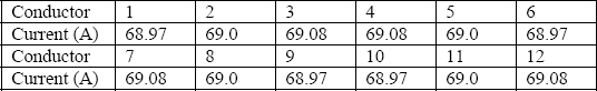
Currents calculated by the method are given in Table 4.1. The currents in parallel conductors are almost equal. The total loss (I² R + circulating current loss) calculated by the above method based on the multi-winding transformer theory is 21.882 kW (for all 3 phases) out of which the I² R loss is 21.87 kW. Thus, the circulating current loss is 12 watts, which is just 0.055% of the I² R loss, suggesting that the transposition scheme is good enough to reduce substantially the circulating current loss. Hence, it can be used for small rating transformers with low radial fields in windings as mentioned earlier. We had calculated for the same transformer the circulating current loss by the method of Rabins and Cogbill as

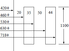
Figure 4.16 Details of 10 MVA transformer.

Table 4.1 Current Distribution in Parallel Strands

P_cc = 0.0206 P_eddy.

The total eddy loss in the LV winding can be determined using Equation 4.99.

$P_{eddy}=\frac{{\omega }^2{t}^2}{24\rho }\frac{B_{gp}^2}{3}\times volume$

$B_{gp}=\sqrt{2}\frac{{\mu }_{0}NI}{H_w}=\sqrt{2}\frac{4\pi \times {10}^{-7}\times 85\times 836.74}{11}=0.1149\text{T}$

$\therefore P_{eddy}=\frac{{(2\pi \times 50)}^2{(0.0023)}^2}{24\times 0.0211\times {10}^{-6}}\frac{{0.1149}^2}{3}\times 0.1079=489.55\text{W}.$

Hence,

$P_{cc}=0.0206\times 489.55=10\text{W}.$

The above answer matches closely with that calculated from the method based on the multi-winding transformer theory (12 W).

4.6.3    FEM analysis

As mentioned earlier, the analytical methods which consider only the axial leakage field are approximate. The effect of radial fields at winding ends or at tap breaks on circulating currents cannot be accounted by these methods. Also, the effect of circulating currents on the main leakage field is neglected. These effects are dominant in large power transformers as well as low-voltage high-current transformers (e.g., furnace transformers). Hence, for more accurate estimation of the circulating current loss and for arriving at a good transposition scheme, a numerical method such as FEM is used [28, 29].

In [29], it has been concluded that in the case of windings without any transpositions or with inadequate transpositions, the analytical formulations give much higher and inaccurate circulating current losses. This is particularly true when the number of parallel conductors is more. This is due to the fact that in such cases, the effect of the field due to large circulating currents significantly affects the leakage field, and this effect is neglected in the analytical formulations.

In the FEM analysis, a time-harmonic formulation is used and all conductors are modeled. It requires a considerable amount of modeling efforts. The conductors are defined as stranded meaning that the eddy currents in them are neglected. Hence, the loss given by FEM analysis is the total of the I² R loss and the circulating current loss. In [30], the circulating currents and the corresponding losses have been calculated for a continuous disk LV winding with 12 parallel conductors by using 2-D FEM analysis and the analytical method based on the multi-winding transformer theory described earlier. The impedance voltage is applied to its HV winding which is modeled as one rectangular block with the definition of the ampere-turn density. The transposition scheme of this winding was not good. The currents calculated by both methods are close, and are compared in Figure 4.17. The circulating current losses calculated by the two methods are also in agreement. When the transposition scheme was changed to the ideal one, in which each of the twelve parallel conductors occupied the original position of every other conductor over an equal distance, the load loss of the transformer reduced by an amount close to the calculated value of the circulating current loss, thus verifying the results of the calculations by the two different methods.

In [17, 18], leakage field distribution is obtained by 3-D FEM analysis. The voltages that circulate currents between parallel conductors are determined by integrating the flux density components over the three dimensions taking into account the transpositions between parallel conductors.

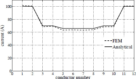
Figure 4.17 Currents in conductors of a continuous disk winding.

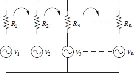
Figure 4.18 Equivalent circuit for calculation of circulating currents.

Based on these voltages and the resistances of the conductors, the circulating currents in the corresponding loops are calculated from the solution of the circuit shown in Figure 4.18. The path of circulating currents is assumed to be resistive because of low values of inductances between parallel conductors (due to adequate transpositions), small spacings between the conductors, and the one-turn path of the currents. It is reported in [17] that a significant reduction in circulating current losses can be achieved by deciding correct locations of transpositions based on such 3-D field calculations.

Until now, we considered only radially placed parallel conductors. There can be axially placed parallel conductors also. If the radial field is symmetrical at both ends and if there are two parallel conductors placed axially as shown in Figure 4.19, the net leakage field enclosed by the loop formed by the two conductors is zero (since the radial field is in opposite directions at the top and bottom ends of the winding). Hence, there will not be any circulating currents on account of the radial field, obviating any need of transpositions in the axial direction. If the radial field is significantly different at the top and bottom ends, the axial transpositions (i.e., exchanging of axial positions) may be required at pre-determined locations determined using FEM. For this case, the approximate analytical formulations, which consider only axial field, cannot be used.

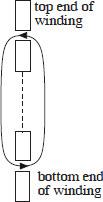
Figure 4.19 Axially placed parallel conductors in a winding.

References

1.    Stoll, R. L. The analysis of eddy currents, Clarendon Press, Oxford, 1974.

2.    Hayt, W. H. Engineering electromagnetics, McGraw-Hill Book Company, Singapore, 1989, pp. 336–363.

3.    Dexin, X., Yunqiu, T., and Zihong, X. FEM analysis of 3-D eddy current field in power transformer, IEEE Transactions on Magnetics, Vol. 23, No. 5, May 1987, pp. 3786–3788.

4.    Holland, S. A., O’Connell, G. P., and Haydock, L. Calculating stray losses in power transformers using surface impedance with finite elements, IEEE Transactions on Magnetics, Vol. 28, No. 2, March 1992, pp. 1355–1358.

5.    Macfadyen, K. A. Vector permeability, Journal IEE, Vol. 94, Pt. III, 1947, pp. 407–414.

6.    Subbarao, V. Eddy currents in linear and nonlinear media, Omega Scientific Publishers, New Delhi, 1991.

7.    Agarwal, P. D. Eddy current losses in solid and laminated iron, AIEE Transactions, Vol. 78, May 1959, pp. 169–181.

8.    Hammond, P. Applied electromagnetism, Pergamon Press, Oxford, 1971.

9.    Turowski, J., Turowski, M., and Kopec, M. Method of three-dimensional network solution of leakage field of three-phase transformers, IEEE Transactions on Magnetics, Vol. 26, No. 5, September 1990, pp. 2911–2919.

10.  Bean, R. L., Chackan, N., Moore, H. R., and Wentz, E. C. Transformers for the electric power industry, McGraw-Hill Book Company, New York, 1959, pp. 396–402.

11.  Boyajian, A. Leakage reactance of irregular distributions of transformer windings by method of double Fourier series, AIEE Transactions — Power Apparatus and Systems, Vol. 73, Pt. III-B, 1954, pp. 1078–1086.

12.  Rabins, L. Transformer reactance calculations with digital computers, AIEE Transactions — Communications and Electronics, Vol. 75, Pt. I, 1956, pp. 261–267.

13.  Andersen, O. W. Transformer leakage flux program based on finite element method, IEEE Transactions on Power Apparatus and Systems, Vol. PAS-92, 1973, pp. 682–689.

14.  Kulkarni, S. V., Gulwadi, G. S., Ramachandran, R., and Bhatia, S. Accurate estimation of eddy loss in transformer windings by using FEM analysis, International Conference on Transformers, TRAFOTECH-94, Bangalore, India, January 1994, pp. I7–I10.

15.  Kulkarni, S. V. and Ramachandrudu, B. Orthogonal array design of experiments for analysis of key performance parameter of transformer, First World Congress on Total Quality Management, Organized by Royal Statistical Society and Sheffield Hallam University, Sheffield, U.K., 10-12 April 1995, pp. 201–204.

16.  McWhirter, J. H., Oravec, J. J., and Haack, R. Computation of magnetostatic fields in three dimensions based on Fredholm integral equations, IEEE Transactions on Magnetics, Vol. MAG-18, No. 2, March 1982, pp. 373–378.

17.  Girgis, R. S., Yannucci, D. A., and Templeton, J. B. Performance parameters of power transformers using 3D magnetic field calculations, IEEE Transactions on Power Apparatus and Systems, Vol. PAS-103, No. 9, September 1984, pp. 2708–2713.

18.  Girgis, R. S., Scott, D. J., Yannucci, D. A., and Templeton, J. B. Calculation of winding losses in shell form transformers for improved accuracy and reliability — Part I: Calculation procedure and program description, IEEE Transactions on Power Delivery, Vol. PWRD-2, No. 2, April 1987, pp. 398–410.

19.  Kozlowski, M. and Turowski, J. Stray losses and local overheating hazard in transformers, CIGRE 1972, Paper No. 12-10.

20.  Mullineux, N., Reed, J. R., and Whyte, I. J. Current distribution in sheet and foil wound transformers, Proceedings IEE, Vol. 116, No. 1, January 1969, pp. 127–129.

21.  El-Missiry, M. M. Current distribution and leakage impedance of various types of foil-wound transformers, Proceedings IEE, Vol. 125, No. 10, October 1978, pp. 987–992.

22.  Turowski, J. Additional losses in foil and bar wound transformers, IEEE PES Winter Meeting and Symposium, New York, January 25-30, 1976, Paper No. A-76-151-1.

23.  Genon, A., Legros, W., Adriaens, J. P., and Nicolet, A. Computation of extra joule losses in power transformers, ICEM 88, pp. 577–581.

24.  Ram, B. S. Loss and current distribution in foil windings of transformers, Proceedings IEE — Generation, Transmission and Distribution, Vol. 145, No. 6, November 1998, pp. 709–716.

25.  Kaul, H. J. Stray current losses in stranded windings of transformers, AIEE Transactions, June 1957, pp. 137–149.

26.  de Buda, R. G. Winding transpositions for electrical apparatus, U. S. Patent No. 2710380, June, 1955.

27.  Rothe, F. S. An introduction to power system analysis, John Wiley, New York, 1953, pp. 45–50.

28.  Isaka, S., Tokumasu, T., and Kondo, K. Finite element analysis of eddy currents in transformer parallel conductors, IEEE Transactions on Power Apparatus and Systems, Vol. PAS-104, No. 10, October 1985, pp. 2731–2737.

29.  Koppikar, D. A., Kulkarni, S. V., Ghosh, G., Ainapure, S. M., and Bhavsar, J. S. Circulating current loss in transformer windings, Proceedings IEE — Science, Measurement and Technology, Vol. 145, No. 4, July 1998, pp. 136–140.

30.  Kulkarni, S. V., Palanivasagam, S., and Yaksh, M. Calculation of circulating current loss in transformer windings using FE analysis, ANSYS Users Conference, Pittsburgh, USA, August 27-30, 2000.