
CHAPTER 4
Work Sharing and Domain Decomposition
In this chapter we consider the distribution of workload across a number of UPC SPMD threads by decomposing the data across the threads that are executing. Distributing work across a number of threads (or processes) in a parallel application requires that each thread have the ability to identity itself through an id value and to recognize the other threads, possibly remote, available to cooperate on performing the application task. This self-identification and recognition of the other cooperating threads allows a division of labor by identifying the partition of the data that will be manipulated by each thread. In UPC, variable declarations establish the affinity of data and threads, providing locality information and control to programmers for decomposing their workload more intelligently. UPC programmers can take advantage of this knowledge by assigning each thread to apply its work, as appropriate, on the data that has affinity to that thread. In this way, the majority of the accesses can become thread local. On machines with physically distributed memory, it is expected that compilers will attempt to co-locate each thread and the data that has affinity to it onto the same physical node, thereby reducing remote accesses and improving execution time. Moreover, as in other parallel programming paradigms, UPC offers the ability for each thread to identify itself and the rest of threads available to help through the special constants MYTHREAD and THREADS, respectively, where MYTHREAD is in the range 0 through THREADS-1.
In addition to the aforementioned basic methods for work sharing, UPC features the iteration statement upc_forall, which distributes independent iterations across threads for parallel execution in different ways. In this chapter we cover these work-sharing concepts and their relationship to affinity of data, to show programmers how to exploit access locality. We also explore how this can be done in the context of blocked shared data structures through application examples that require interesting data distributions such as multidimensional arrays and trees.
4.1 BASIC WORK DISTRIBUTION
Consider a version of the matrix-vector multiplication example of Examples 2.2 and 2.3, in which a matrix of THREADS *10 × THREADS is multiplied by a vector of length THREADS. Knowing the number of threads, THREADS, the matrix and vector dimensionalities, and given that each thread can identify itself through the special constant MYTHREAD, work can be distributed such that each thread operates on a unique set of rows from the matrix a[][].
Example 4.1: matvect3.upc
#include <upc_relaxed.h>
shared [THREADS] int a [THREADS*10][THREADS];
shared int b [THREADS], c [THREADS*10];
int main (void)
{
  int i, j;

  for(i = MYTHREAD; i < THREADS*10; i += THREADS)
  {
    c [i] = 0;
    for (j = 0; j < THREADS; j++)
      c [i] += a [i][j]*b [j];
  }

  return 0;
}
In this example, matrix a [][], which has the dimensionality THREADS*10 × THREADS, is multiplied by vector b [], which is of length THREADS, producing vector c [], which is of length THREADS*10. The declarations
shared [THREADS] int a [THREADS*10][THREADS];
shared int b [THREADS], c [THREADS*10];
establish a [][], b [], and c [] as shared arrays. Further, the a [][] array is distributed in blocks of one row across the threads (i.e., each thread gets one row in round-robin fashion). At the end, each thread ends up with 10 rows in its local shared space when all THREADS*10 rows are distributed.
As the loop
for(i=MYTHREAD; i < THREADS*10; i+=THREADS)
is executed by all threads concurrently in SPMD style, each thread operates at first on the row of matrix a [][] that matches the thread number. Then each thread jumps by THREADS row to work with its next row, and so on, until all 10 rows are processed.
In performing the operations above, it should be noted that each thread operates on the a-elements that are local to it only. Thus, the inherent locality in the underlying problem is fully exploited. This is generally much easier to do in UPC than in many other paradigms. Note also that one can distribute the matrix in blocks of 10 rows each. This is done by changing the matrix a [][] declaration to
shared [THREADS*10] int a [THREADS*10][THREADS];
The outer loop may then be slightly changed in order to continue to exploit locality and maintain the execution efficiency and good performance, but the remainder of the program remains unchanged.
4.2 PARALLEL ITERATIONS
In Section 4.1 we demonstrated how work can be distributed and how each thread can determine what its assigned share of work is based on MYTHREAD, THREADS, and the layout of shared data. Using these constructs and methods, it was demonstrated that a programmer can easily distribute work such that each thread can work as much as possible on data that has affinity to it, thereby maximizing data locality exploitation.
Another powerful UPC construct for specifying program parallelism is upc_forall, which simplifies this process and provides many options for defining workload distribution across threads. The upc_forall construct is a work-sharing iteration statement, which syntactically resembles the C for loop statement. It assumes, however, that all iterations are independent of one another and therefore can be thought of as units of work that can be distributed across the threads, where they get executed in parallel. The syntax for upc_forall is as follows:
upc_forall( expression1; expression2; expression3; affinity)
The first three arguments of the upc_forall statement, expression1, expression2, and expression3, are all expressions. The typical use of these is similar to that of the C for statement: that is, initialization, test, and update. Any of these expressions can be omitted, but the semicolons cannot be removed.
The fourth component of the upc_forall construct, affinity, is the controlling element that determines which thread executes a given iteration. Thus, affinity must have a unique value in each thread. Each iteration is executed by exactly one thread, but one thread can execute more than one iteration. To this end, the affinity component can be either an expression or a pointer-to-shared. When affinity is an integer expression, all iterations for which the value “affinity modulo THREADS” matches the thread number of a given thread, MYTHREAD, will be executed by that thread. In other words, the loop body of the upc_forall statement is executed for each iteration in which the value of MYTHREAD equals the value “affinity modulo THREADS.” When affinity is of pointer-to-shared type, a thread executes a given iteration if the object pointed to has affinity to that thread (i.e., if the object pointed to was local to that thread). In other words, the loop body of the upc_forall statement is executed for each iteration in which the value of MYTHREAD equals the value of upc_threadof (affinity).
Consider a variant of the matrix-to-vector multiplication in which the blocked matrix has a dimensionality of THREADS*4 × THREADS*4, and each block is of size THREADS*4.
Example 4.2: matvect4.upc
#include <upc_relaxed.h>
shared [THREADS*4] int a[THREADS*4][THREADS*4];
shared int b[THREADS*4], c[THREADS*4];

int main (void)
{
  int i, j;

  upc_forall(i = 0; i < THREADS*4; i++; i)
  {
    c [i] = 0;
    for (j= 0 ; j < THREADS*4 ; j++)
      c [i] += a [i][j]*b [j];
  }

  return 0;
}
In this case, the affinity expression is simply i. This affinity expression distributes the iterations in round-robin fashion across the threads. All iterations for which i modulo THREADS equals some integer k will be executed by thread number k, where k ranges from 0 to THREADS-1. As the upc_forall construct is the outer iteration statement in this example, each iteration corresponds to the processing of one row of matrix a [][]. The data layout selected distributes the matrix by rows, one row per thread in round-robin fashion, ensuring that all accesses to the a [][] matrix are local.
The foregoing scenario can be accomplished by using the affinity field as a pointer-to-shared. The only change needed is as follows.
The affinity field is basically a pointer to the first element of the ith row in matrix a [][]. Alternatively, a [i] can also be used. However, some early compilers may not support this syntax, so &a [i][0] is used.
In Example 4.3, data is distributed by blocks of one row each, in round-robin fashion. Each thread has four noncontiguous rows assigned to it. In some applications it could be better to distribute an array in groups of contiguous rows. To continue to harness the benefit of locality, equivalent chunks of iterations need to be assigned to the same thread. Consider modifying Example 4.3 to distribute data by chunks of four rows and assign every four consecutive iterations to one thread.
Example 4.4: matvect6.upc
#include <upc_relaxed.h>


shared [THREADS*16] int a[THREADS*4] [THREADS*4];
shared int b [THREADS*4], c [THREADS*4];

void main (void)
{
  int i, j;


  upc_forall(i = 0; i < THREADS*4; i++; (i/4))
  {
    c [i]= 0;
    for (j= 0; j < THREADS*4;j++)
      c [i]+ = a [i][j]*b [j];
  }
}
The affinity is an expression in this case, which is the integer division of the current iteration number by 4, to produce one thread number for every four consecutive iterations. In addition to being an integer expression or a pointer-to-shared, the affinity field in a upc_forall statement can be either continue or left empty. In these cases, all iterations are executed by all threads. Like the ISO C for statement, the UPC upc_forall construct may be nested within the program structure either directly or through function calls. In this case the outermost upc_forall, which does not have continue, or empty affinity, is considered the controlling upc_forall. All of its inner upc_forall loops will act as if they have a continue or an empty affinity field, and all of their iterations will therefore be executed by all threads. The utility of these cases is quite limited. Therefore, interested readers should refer to the language specifications for more details.
4.3 MULTIDIMENSIONAL DATA
As an extension of ISO C, UPC stores two-dimensional data in a row-major order and maintains the ability of pointers to address multidimensional data as linear arrays. To ensure that a pointer-to-shared traverses both the elements of an array and the elements of a block in a consistent manner, data blocks are limited to be only one-dimensional. However, there are some methods, which are not very straightforward, for distributing multidimensional data blocks (discussed later). In this section we show how multidimensional data can be accessed effectively using basic UPC data distributions methods. This can be done conveniently and may even achieve better performance than distributions with traditional multidimensional blocks.
In these examples, such as Example 4.4, we distributed a matrix by groups of rows. In addition to the benefit of having a consistent way to traverse the blocks and the overall matrix using the same pointer-to-shared variable, this type of distribution can potentially limit the number of remote transactions because one-dimensional blocks create fewer ghost zones when neighboring data is needed. In general, the number of ghost zones is typically twice the number of dimensions of the block used, and the number of ghost zones typically determines the number of data transfers. The volume of remote data elements may be the same in both cases. However, most parallel architectures perform fewer transfers with more data per transfer more efficiently than do larger number of transfers with fewer data per transfer. Therefore, one-dimensional blocking lends itself to higher performance than do multidimensional distributions.
There are many ways to distribute a three-dimensional array across the threads. Figure 4.1 shows three basic approaches. Figure 4.1a shows the default case in which blocks of one element each are distributed across the threads in round-robin fashion, which can be accomplished by the following declaration:
shared double grid [N][N][N];
Figure 4.1b shows the case of distributing blocks of one row each, which can be established as follows:
shared double [N] grid [N][N][N];
and for the distribution of Figure 4.1c which distributes data by blocks of two-dimensional faces, the declaration is
shared double [N*N] grid [N][N][N];
Again, the preceding cases are only examples; many other declarations can be used to distribute data in other ways that are derived from the linear distribution offered by UPC, such as distributing by chunks of rows or multiple faces across the threads. The declarations are only one part of how to handle multidimensional arrays and multidimensional cells. Another aspect is how to access and address the data. It is important here to note that the cell and the block do not need to be the same. The cell is simply the smallest possible entity to which application physics or computational laws are applied. The block is a data distribution unit. Although our next example will demonstrate the distributions in the previous declarations, it should be noted that having more cells per block can contribute to improved performance.

Figure 4.1 Multidimensional Data and Cells
To examine multidimensional data handling in UPC, we consider the three-dimensional heat conduction problem [NTM04] in which the three-dimensional partial differential equation in a stationary medium is

where T is temperature, t is time, and α is the thermal diffusivity. For simplicity, we assume that the source remains hot and that its thermal properties are constant. In addition, we also assume that the entire medium is a solid with thermal diffusivity, α, of 1.0. Inside a three-dimensional cell, based on (1), the temperature is calculated as follows:

Figure 4.2 Basic Stencil Operations for the Heat Transfer Problem
![]()
which is the basic, stencil operation, illustrated in Figure 4.2.
The following is the code for main() and initialize().
Example 4.5: heat_conduction1.upc
1. #include <stdio.h>
 2. #include <math.h>
 3. #include <upc_relaxed.h>
 4. #include "globals.h"

 5. // Declare two global grids, either source or
       destination at
 6. // each epoch, with the data distribution as described in
 7. // globals.h
 8. shared [BLOCKSIZE] double grids [2][N][N][N];
 9. shared double dTmax_local [THREADS];

10. void initialize(void)
11. {
12.   int y, x;

13.   /* sets one edge of the cube to 1.0 (heat) */
14.   for(y=1; y<N-1; y++)
15.   {
16.     upc_forall(x=1; x<N-1; x++; &grids [0][0][y][x])
17.     {
18.       grids [0][0][y][x]= grids [1][0][y][x]= 1.0;
19.     }
20.   }
21. }

22. int main(void)
23. {
24.   double dTmax, dT, epsilon;
25.   int finished, z, y, x, i;
26.   double T;
27.   int nr_iter;
28.   int sg, dg; // stands for source grid and destination
        // grid indexes

29.   initialize();

30.   /* sets the constants */
31.   epsilon = 0.0001;
32.   finished = 0;
33.   nr_iter = 0;
34.   sg = 0;    // using grids [0][][][] as source array
35.   dg = 1;    // using grids [1][][][] as destination array

36.   /* synchronization */
37.   upc_barrier;

38.   do
39.   {
40.     dTmax = 0.0;
41.     for(z=1; z<N-1; z++)
42.     {
43.       for(y=1; y<N-1; y++)
44.       {
45.        upc_forall(x=1; x<N-1; x++; &grids [sg][z][y][x])
46.         {
47.          T = (grids [sg][z+1][y][x]+ grids [sg][z-1][y][x]+
48.            grids [sg][z][y-1][x]+ grids [sg][z][y+1][x]+
49.            grids [sg][z][y][x-1 + grids [sg][z][y][x+1])/6.0;
50.          dT = T - grids [sg][z][y][x];
51.          grids [dg][z][y][x]= T;

52.          if(dTmax < fabs(dT))
53.            dTmax = fabs(dT);
54.         }
55.       }
56.     }

57.     dTmax_local [MYTHREAD] = dTmax;
58.     upc_barrier;

59.     dTmax = dTmax_local [0];
60.     for(i=1; i<THREADS;i++)
61.       if(dTmax < dTmax_local [i])
62.         dTmax = dTmax_local [i];
63.     upc_barrier;

64.     if(dTmax < epsilon)
65.       finished = 1;
66.     else
67.     {
68.       // swapping the source and destination “pointers”
69.       dg = sg;
70.       sg = !sg;
71.     }
72.     nr_iter++;
73.   } while(!finished);

74.   upc_barrier;

75.   if(MYTHREAD == 0)
76.   {
77.    printf(“%d iterations
”, nr_iter);
78.   }

79.     return 0;
80. }
To set up the problem size and data layout used, a globals.h include file is created (line 4) which could at minimum have
#define N 32
Together with the size of the array, this include file specifies one of the three data distributions depicted in Figure 4.1. This is accomplished by setting the constant BLOCKSIZE through a preprocessor macro definition using one of the following:
#define BLOCKSIZE 1
#define BLOCKSIZE N
or
#define BLOCKSIZE N*N
which would distribute data in equal blocks across all the threads. In this case two cubic grids are needed, one grid for holding the data from the preceding iteration while the new data for the current iteration is written into the other grid. To simplify the process, rather than declaring two shared three-dimensional arrays separately, line 8 declares a four-dimensional shared array, grids, of 2 × N × N × N dimensionality which can hold both arrays. The array is distributed by blocks as defined in the header file, globals.h. Thus, the first three-dimensional array can be indexed as grids [0][z][y][x], while the second is indexed as grids [1][z][y][x]. The declaration is external since shared arrays cannot have dynamic scope. The variables sg and dg, declared in line 28 and initialized to 0 and 1 in lines 34 and 35, respectively, are used in the first index position to determine which of the two cubes is the source grid and which is the destination grid during a given iteration. They are also used to swap this role, of source and destination grids, at the end of each iteration according to lines 69 and 70.
Boundary conditions are introduced at one face of each N × N × N grid through the function initialize(), lines 10 through 21. We assume in this case that N is divisible by THREADS. Thus, each of the threads initializes one row in surface in parallel. From the multiple assignments of line 18, this initialization is carried out for both grids simultaneously.
The simulation proceeds iteratively until the maximum change in temperature falls below a given threshold, epsilon, line 24. Line 24 also declares the private variables dT to hold the current change of temperature and dTmax to search for a local maximum change of temperature. The declaration in line 9 is for a shared array, dTmax_local[], that has one element per thread to hold the local maximum temperature change into a shared array to simplify finding the global maximum change in temperature, lines 59 through 62. However, barrier synchronization is applied in line 58 to ensure that all threads have deposited their local maximum temperature change into that array before a global maximum is computed. The barrier present in line 63 ensures that all threads have gone through the shared dTmax_local [] and determined the maximum value, allowing the threads to reuse the dTmax_local [] buffer for the next iteration.
The bulk of work takes place between lines 38 and 73, and it is started at all threads simultaneously due to the barrier synchronization in line 37. For each z and y coordinate combination, the temperature and change in temperature are computed in parallel for all possible x coordinates using a upc_forall operation. From the affinity expression, each iteration is executed by the thread that has the target data point locally. If the grids array is distributed by the largest possible block size, most of the data accesses associated with this computation could be local. This example demonstrates that although the array data was not distributed by three-dimensional blocks, accesses were straightforward. The reason is that the shared memory view of UPC makes dealing with the arrays similar to that of the sequential code. Meanwhile, the data distributions selected at declaration time, along with an adequate selection of the affinity field in the upc_forall statement, maximize locality exploitation. When all threads are done as determined by the barrier synchronization in line 74, thread 0 prints the number of iterations.
Example 4.5 demonstrated the ease and efficiency of dealing with higher-dimensional arrays in UPC. Here, we address how to partition the data into three-dimensional blocks of equal sizes across the threads, which is commonly used in message-passing codes. We then show how to modify Example 4.5 to adopt this new strategy. The discussion is limited to cases where the number of threads is a power of 2, and the number of elements in the array is divisible by the number of threads for simplicity. Examples of the target distribution are shown in Figure 4.3. Given a particular number of threads, Figure 4.3 shows how an array can be distributed such that each thread ends up with an equal-sized three-dimensional cell. The partitioning of Figure 4.3 can be determined recursively and it is commonly referred to as recursive bisection, where the number of cells doubles as the number of threads doubles. The partitioning for each number of threads is described uniquely by a number of columns, a number of rows, and a number of planes, as shown in Figure 4.3.

Figure 4.3 Partitioning Using Recursive Bisection of Three-Dimensional Arrays into Equal Three-Dimensional Cells Across the Threads
This type of data decomposition is often used in message-passing paradigms. For example, it is used in the MPI-FORTRAN version of the CG workload of the NAS Parallel Benchmark NPB-2.4 [NPB03]. There, for each power-of-2 number of threads, the grid is split in half, column-wise, row-wise, and then plane-wise, respectively, or simply across the x, y, then z coordinates. Such grid decomposition is creating the biggest squared three-dimensional cells. Due to the static nature of the arrays, these parameters should all be computed ahead of time and inserted into a header file. In C, this domain decomposition (i.e., data partitioning parameters) can be computed as follows.
Example 4.6: initialize.c
NO_COLS = NO_ROWS = NO_PLANES = 1;
j = 0;
for(i=2; i<=THREADS; i<<=1)
{
  if((j%3)==0)
    NO_COLS *= 2;
  else if((j%3)==1)
    NO_ROWS *= 2;
  else
    NO_PLANES *= 2;
  j++;
}
After precomputing the partitioning parameters (number of rows, columns, and planes), the dimensionality of the cells in terms of array elements is determined as follows:
DIMX = N / NO_COLS;
DIMY = N / NO_ROWS;
DIMZ = N / NO_PLANES;
The values for DIMX, DIMY, and DIMZ should then be placed in globals.h. In fact, it is even possible to create a small program that determines the partitioning parameters and also creates the inclusion file, populating it with the dimensionality of the cells, which is the case in NPB-2.4 [NPB03].
Now consider modifying the previous heat transfer program to use this new data partitioning strategy. First, we replace the grids [][][][] declaration.
Example 4.7: heat_conduction2.upc
#define CELL_SIZE DIMZ*DIMY*DIMX

struct gridcell_s {
  double cell[CELL_SIZE];
};
typedef struct gridcell_s gridcell_t;

shared gridcell_t cell_grids [2][THREADS];

#define grids(gridno, z, y, x)
cell_grids [gridno][((z)/DIMZ)*NO_ROWS*NO_COLS +
((y)/DIMY)*NO_COLS +((x)/DIMX)].cell [((z)%DIMZ)*DIMY*DIMX +
((y)%DIMY)*DIMX + ((x)%DIMX)]
In this code, gridcell_s is a structure that holds all the elements of one cell in a one-dimensional array, while cell_grids [2][THREADS] is a two-dimensional array of two rows and THREADS columns, one row for the source grid and the other for the destination grid. Indexing these two virtual three-dimensional arrays properly is accomplished by the macro grids(no,z,y,x). Therefore, the rest of the program should then use the macro grids(no,z,y,x) instead of grids [no][z][y][x].
4.4 DISTRIBUTING TREES
Trees are commonly used in a searching problem. In this section we consider distributing a tree search through an example, which considers an instance of the N-queens problem. The tree in this case will have a simple representation that is appropriate to the problem. The focus is on how to distribute the search space across the threads. Working with trees represented as linked lists is treated in Chapter 7.
Sequential N-Queens
The N-queens problem is a classic problem in computer science, due to its interesting computational behavior, depth-first searching and backtracking, and the fact that its processing time grows at a nonpolynomial (NP) rate. Thus, as the problem size grows, the execution time grows at a much more dramatic pace. There are numerous variations of the problem description. In this version of the problem, we seek to find all solutions to the problem of placing N queens on an N × N chessboard such that no queen can kill the other. This implies that no two queens can be placed on the same row, column, or along the same diagonal.
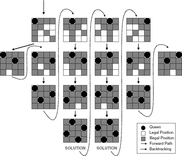
Figure 4.4 Sequential N-Queens Algorithm
Figure 4.4 shows the computational flow in the N-queens problem using a simple example of a 4 × 4 chessboard. In this figure the solid arrows represent moves along a search path and the dotted lines represent backtracking after a solution was found or it was determined that the previous path was not going to lead to a solution. The solid black circles indicate queens positioned on the board. Also, a shaded box means a position that can no longer be used by a queen or it will be killed; a white box indicates an open position that can still be used. The algorithm starts by placing the first queen in the first column of the first row, then shading all boxes along the same row, column, or diagonal. Then we attempt to place the second queen in the second row in the first open position. It is clear after placing the second queen that no more queens can be placed on the board; therefore, this path was abandoned and we had to back-track to where a queen was placed in the second column of the first row. The algorithm continues, and at the end it is apparent that only two valid solutions, in which all four queens can be safely placed, exist.
One possible program implementation is to use one data structure to represent, in a binary format, the constraints associated with all prior queen placements. Another data structure can then be used to represent the new constraints that are to be created with the placement that we are about to make. Let us call these data structures vrlnbl_cells, unsafe_cells, and next_row_unsafe, respectively, and note that they will all use similar data structures. Figure 4.5 shows the data structure that can be used for mask_t, which is simply an integer, for the case of the 4 × 4 chessboard.

Figure 4.5 Representing Potential Conflicts
The information is coded in binary, where in each binary cell a “1” means an invalid position that can cause death to the new queen and “0” means a safe position. In each 4-bit field (e.g., the conflicts with columns), the leftmost cell is used to indicate the fourth column and the rightmost indicates column 0. Figure 4.6 shows how these representations work. There are three types of information to be kept track of: the current state of unsafe cells due to queens that have already been placed (unsafe_cells), the vulnerable cells from which danger could be paused for a contemplated queen placement (vrlnbl_cells), and the danger map associated with the placement of queens in the next row (next_row_unsafe). Figure 4.6 gives a few snapshots into the algorithm operation as it unfolds, using this binary representation of potential conflicts.

Figure 4.6 Snapshots into the N-Queens Algorithm
Example 4.8: nqueens1.c
1. typedef uint64_t mask_t; // should be big enough for 3*N bits 2. int N, no_solutions=0; 3. mask_t basemask, leftdiagmask, centermask, rightdiagmask; 4. void Nqueens(int cur_row, mask_t unsafe_cells) 5. { 6. int col; 7. mask_t vrlnbl_cells, next_row_unsafe; 8. if(cur_row == N) 9. { 10. no_solutions++; //Increment the number of valid // solutions 11. return; 12. } 13. for(col=0; col<N; col++) 14. { 15. vrlnbl_cells = basemask<<col; // Place queen on row 16. if(unsafe_cells& vrlnbl_cells) 17. continue; // CONFLICT! 18. // No conflicts here, create the unsafe_cells mask for // the next row 19. // next_row_unsafe = unsafe_cells | vrlnbl_cells; 20. // next_row_unsafe =((next_row_unsafe&leftdiagmask)>>1 // left | (next_row_unsafe¢ermask) // center | ((next_row_unsafe&rightdiagmask)<<1); // right diagonals 21. Nqueens(cur_row+1, next_row_unsafe); 22. } 23. } 24. int main(int argc, char **argv) 25. { 26. if(argc != 2) 27. {printf(“Usage: %s [N] ”, argv [0]); return;} 28. sscanf(argv [1], “%d”, &N); 29. if(N*3 > 64) 30. {printf(“64bit word not big enough! ”); return;} 31. basemask=1|(1<<N)|(1<<(2*N));leftdiagmask=(1<<N)-1; centermask=leftdiagmask<<N; rightdiagmask= centermask <<N; 32. Nqueens(0, 0); 33. printf(“Total number of solutions for N=%d: %d ”, N, no_solutions); 34. return 0; 35. }
Example 4.8 shows a possible implementation for the sequential N-queens problem for the more general case. Lines 1 through 3 define a number of global variables, such as basemask, which represents the constraints that are to be created by the next queen to place. This variable should be at 3N bits in size for an N × N problem, where the columns, the left diagonal, and the right diagonal require N bits each. In addition, it defines no_solutions, a variable that holds the number of valid solutions at the end of the execution. Lines 4 through 23 define the Nqueens() function itself, and lines 24 and 25 list the main() driver. The main() obtains the size of the problem, N, from the user and sets basemask, based on the desired size of the problem, to 1 in the least significant bit of each of the fields: left diagonals, columns, and right columns, respectively, from right to left. The Nqueens() function is then called once by the main(). The Nqueens() function is recursive and will continue to call itself until it examines all solutions, returning at the end the number of valid solutions that were found, at which point main() prints out that number.
The function Nqueens(), lines 4 through 23, receives two input parameters, cur_row and unsafe_cells. Initially, it is called from main() with these two parameters set to 0, line 32. Thus, placement starts from the first row, with all cells on the chessboard open. Lines 8 through 12 determine whether the entire process is now completed, and if so, it terminates the program. This is done by checking if we have already reached row N, and if we have, it means that N queens have been placed on rows 0 through N – 1 Then the function increments the number of solutions and returns.
The bulk of the work takes place in lines 13 through 22. As each function invocation also specifies a current row, a for loop starting in line 13 simply examines all potential column placements. For each of these columns, a mask to reflect the potential exposed cells to result from this placement is created by shifting the basemask by the column number to the left, line 15. If these new restrictions are in conflict with the restrictions specified by the current state, as represented in mask, a conflict has occurred and been detected, line 17. In this case we simply skip to the next column by jumping to the next loop iteration. If there is no conflict, we compute the unsafe cells for the next row. This is accomplished by integrating the historical unsafe cells and the vulnerable cells of the current queen, then shifting each field appropriately to reflect the threats in the next row, lines 19 and 20. The function then calls itself recursively by advancing the row in question and with a new state for unsafe cells, line 21.
Parallel N-Queens
As the problem size increases, the number of iterations required to search for all possible ways that the N queens can coexist on the same board grows dramatically. Luckily, N-queens lends itself to parallelism. This is because N-queens is a tree-search problem in which the subtrees are independent of one another and therefore can be distributed across a number of processors easily.
Thus, N-queens can benefit from the speed of parallel processing. For example, one possibility is distributing the problem across N threads, where each thread solves the sequential problem for the case where a queen has been placed in one particular column of the first row (Figure 4.7). For larger problems and larger machines, each thread searches along one of the subtrees that correspond to a given row-column position combination in the first L rows. All threads proceed in parallel to perform a sequential search along their own subtrees. Figure 4.8 gives an example of work distribution where each job is based on the position combination of the first two rows. The remote accesses associated with this algorithm are minimal and the parallel algorithm is therefore embarrassingly parallel, which means perfectly parallel with very low communication overhead.
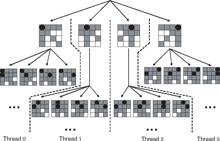
Figure 4.7 N-Queens Problem Using UPC
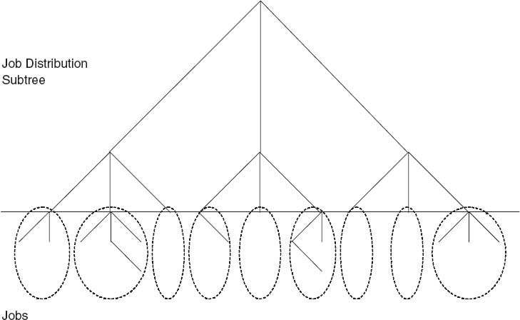
Figure 4.8 N-Queens Job Distribution Tree
Example 4.9: nqueens2.upc
1. #include <upc_relaxed.h>
2. int N, level, no_solutions=0, method=0;
3. shared int sh_solutions[THREADS];
4. mask_t basemask, leftdiagmask, centermask, rightdiagmask;
5. #define ROUND_ROBIN 0
…
6. void do_job(int job, int no_jobs)
7. {
8. int i, j, row, col;
9. mask_t vrlnbl_cells, unsafe_cells;
10. for(j=no_jobs/N, unsafe_cells=0, row=0; j>=1; j/=N,
row++)
11. {
12. col = job%(N*j)/j;
13. vrlnbl_cells = basemask<<col;
14. if(unsafe_cells& vrlnbl_cells)
15. break; // CONFLICT! - ignore job
16. unsafe_cells |= vrlnbl_cells;
17. unsafe_cells = ((unsafe_cells&leftdiagmask)>>1)
| (unsafe_cells¢ermask)
| ((unsafe_cells&rightdiagmask)<<1);
18. if(j == 1)
19. Nqueens(row+1, unsafe_cells);
20. }
21. }
22. void distribute_work()
23. {
24. int i, job, no_jobs;
25. for(i=0, no_jobs=N; i< level; i++)
26. no_jobs *= N;
27. if(method == ROUND_ROBIN)
28. {
29. upc_forall(job=0; job<no_jobs; job++; job)
30. do_job(job, no_jobs);
31. }
32. else
33. {
34. upc_forall(job=0; job<no_jobs; job++;
(job*THREADS)/no_jobs)
35. do_job(job, no_jobs);
36. }
37. }
38. int main(int argc, char **argv)
39. {
40. int i;
41. if((argc != 3) && (argc != 4))
42. {if(MYTHREAD == 0) printf("Usage: %s [N] [lvl] [CHUNK
flag]
", argv[0]); return −1;}
43. sscanf(argv[1], “%d”, &N);
44. sscanf(argv[2], “%d”, &level);
45. if(argc == 3) method = 1; // 3 args, CHUNK method
enabled
46. if(level >= N)
47. {
48. if(MYTHREAD == 0)
49. printf(“lvl should be < N
”);
50. return −1;
51. }
52. if(N*3 > 64)
53. {
54. if(MYTHREAD == 0)
55. printf(“64bit word not big enough!
”);
56. return −1;
57. }
58. basemask=1|(1<<N)|(1<<(2*N)); leftdiagmask=(1<<N)−1;
centermask=leftdiagmask<<N;
rightdiagmask¼centermask<<N;
59. distribute_work();
60. printf(“TH%02d: Total number of solutions for N=%d:
%d
”, N, no_solutions);
61. sh_solutions[MYTHREAD] = no_solutions;
62. upc_barrier;
63. if(MYTHREAD == 0)
64. {
65. for(i=1; i<THREADS; i++)
66. no_solutions += sh_solutions[i];
67. printf(“Total number of solutions: %d
”,
no_solutions);
68. }
69. return 0;
70. }
In Example 4.9 the line numbers are given sequentially for ease of viewing, but be aware that “…” signifies segments of code that are not included, for the sake of brevity. Lines 2 through 4 have some of the key declarations. At line 3 an array of size THREADS is created. This is declared as shared int sh_solutions [THREADS] with a default distribution of [1]. This array is used to store the number of solutions that each thread discovers, where each thread stores the local number of solutions at the corresponding array cell. In addition, level is a row number in the chessboard that is used to determine the level at which the search tree will be segmented into independent subtrees that are to be evaluated by the various threads. The variable method is used to allow the user to specify whether the subtrees should be distributed across the threads by chunks of subtrees or in round-robin fashion.
Lines 46 through 51 ensure that the number of levels at which the tree is to be divided is valid. The jobs are distributed among the threads by the function distribute_work(), which sets the job distribution strategy as chunks or as simple round robin. The solutions are then calculated using the function do_job(), shown in lines 6 through 21. A barrier is placed in line 62 to ensure that all the threads have completed finding all possible solutions. In lines 63 through 68, thread 0 aggregates the number of solutions and prints the result.
4.5 SUMMARY
Work sharing is simply to make each thread able to understand its responsibilities during a parallel program. Domain decomposition typically refers to partitioning the data across the threads in a manner consistent with the duties of each thread. Coming up with effective work-sharing and domain-decomposition strategies requires self-awareness, i.e., each thread should be able to identify itself, (e.g., using MYTHREAD) and awareness of what other threads are there to help, e.g., using THREADS. More convenient constructs to use are also available in UPC, such as upc_forall(). UPC is a locality-aware programming paradigm. Data decomposition is done primarily as a part of the declarations, and workload sharing can easily be planned in way that exploits data locality.
EXERCISES
4.1 Starting from the heat conduction code, develop an edge detection image processing application using the Sobel operators.
4.2 Transform the N-queens problem into a maze problem. Start by developing a sequential version, then parallelize it.
UPC: Distributed Shared Memory Programming, by Tarek El-Ghazawi, William Carlson, Thomas Sterling, and Katherine Yelick
Copyright © 2005 John Wiley & Sons, Inc.