

272 Ultra-Realistic Imaging
Object
(a) Creation of H
1
hologram
(b) H
1
:H
2
transfer process
Object
2
2
?
θ
A
?
(c) Viewing the H
2
Ref beam
Object
Plan view Side view
Plan view Side view
Eye
Object
Diffracted image of H
1
White light illumination
White light illumination
Eye
Diffracted image of H
1
Object beam
Object beam
Object beam
Writing the “red” data Writing the “green” data Writing the “blue” data
h
Ref beam
Ref beam
h
h
H
1
H
1
H
1
?
?
??
?
?
ℱ′
?′
ℱ′
?′
ℱ′
?′
?
H
2
H
2
H
1
reference beam H
1
reference beamH
2
reference beam
H
2
reference beam
h
1
2
2
θ
A
θ
A
z
B
z
B
z
G
z
R
z
G
z
R
H
1
Blue image of red H
1
Red image of blue H
1
Red image of red H
1
+
Blue image of blue H
1
+
Green image of green H
1
H
H
H
H
H
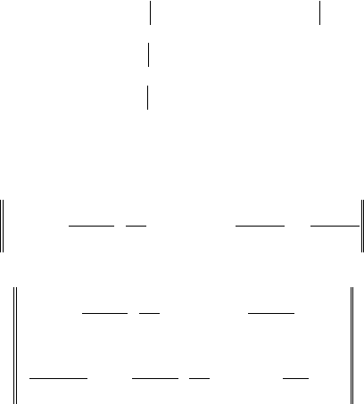
FIGURE 8.17 The creation of an MWDH rainbow master hologram using a single laser: (a) creation of the red, green
and blue H
1
holograms, (b) the H
1
:H
2
transfer using a single colour laser, and (c) viewing the nal H
2
rainbow transmission
hologram. Note the inverting camera and the non-conjugate SLM conguration.

273Digital Holographic Printing: Data Preparation, Theory and Algorithms
Using the results from Chapter 11 (Equation 11.20)* and taking h to be a positive value, we can see that
the rst condition described above is satised (in terms of the following 3 × 2 matrices) when
y
y
y
z
z
z
h
W
R
G
B
R
G
B
R
G
=−
−
()
−
()
λ
λλ θ
λλ
W
W
sin
sinn
sin
θ
λλ θ
λ
λ
λ
B
R
G
B
−
()
W
(8.91)
This implies that the R, G and B H
1
holograms are aligned at an angle equal to the achromatic angle
dened as
θ
A
= tan
−1
(sin θ) (8.92)
where θ represents the angle of reference (and illumination) incidence. To understand the image process-
ing required, we consider two cases: (i) writing the blue H
1
at λ
W
and (ii) how this H
1
replays at λ
B
. With
this in view, we set up separate real Cartesian coordinate systems
()
′′
UV
WW
,
and
()
′′
UV
BB
,
, respectively,
for the projected SLM plane ?ʹ in both cases as illustrated in Figure 8.18. For a test ray written at λ
W
off-
axis to then replay at λ
B
the correct camera data on-axis, we require that
′
=
′
−−
()
′
=
′
−−−
()
Uxhz
Vyyhz
W
H
W
V
B
BB
tan
tan
Ψ
Ψ
2
2
(8.93)
*
Note that we have transformed to the coordinates we are using here which are different from those used in Equation11.20.
h
(a) Side view
2
ξ
y
B
y
B
+
(h–|z
B
|)tan( )
Ψ
V
2
(h–|z
B
|)tan( )
Ψ
H
2
z
B
V'
W
V'
B
=y'
U'
B
=x'
U'
W
z
B
2
(b) Plan view
H
1
on recording at λ
W
H
1
on recording at λ
W
H
1
on replay at λ
B
H
1
on replay at λ
B
H
2
ref beam
h
?
?
ℋ
ℋ
ℱ´
?´
ℱ´
?´
FIGURE 8.18 Coordinate systems
()
′′
UV
WW
,
and
()
′′
UV
BB
,
characterising the projected SLM plane showing rays at off-
axis recording (λ
W
) and on-axis replay (λ
B
) for (a) side view and (b) plan view.

274 Ultra-Realistic Imaging
We must then be careful to discretise the
′′
()
UV
WW
,
system in the following way:
′
=
′
−
()
−
′
=
′
−
()
−
U
z
N
V
z
N
W
M
H
W
V
21
12
21
1
B
B
µ
ν
tan
t
Ψ
aan
Ψ
V
2
(8.94)
This takes into account the fact that the effective eld of view of the printer objective is decreased on
replay due to the change in wavelength. This then leads us, with the help of Equations 8.88 and 8.91, to
the index rules between (i′, j′) and (μ′, v′):
′
=+
′
−
()
+
−
()
−
()
′
=+
′
−
()
i
N
j
W
MW
W
W
11
1
2
11
λ
λ
µ
λλ
λ
λ
λ
ν
B
B
B
++
−
()
−
()
+
N
VW
W
V
1
2
1
2
λλ
λ
θ
B
sincot
Ψ
(8.95)
We may now convert these equations to relations for the un-primed integers (i,j,μ,ν) by application of
the inverting camera Equation 8.27 and the corresponding relations for a non-conjugate SLM—μ′ =
N
M
− μ + 1 and ν′ = N
V
− ν + 1. Finally we can use these index laws and Equation 8.89 with NB = 1 to
arrive at the following transformation:
µν
α
α
µµ µααα
νν ν
SI
C
ij
C
MA
V
NN
NC
=∈≤
{}
∈≤
{}
∈≤
{}
∀∀
∀∀
CC ∈
{}
{}
=
R,G,B
otherwise0
(8.96)
where
iN N
N
jN N
M
W
M
MWC
W
V
W
V
=− −+
−
()
−
()
=− −
λ
λ
µ
λλ
λ
λ
λ
ν
C
C
()
()
1
2
++
−
()
−
()
+
N
VWC
W
V
1
2
1
2
λλ
λ
θsincot
Ψ
(8.97)
We have omitted the subscript β from S on purpose, as this transformation describes R, G and B H
1
slit
holograms only one hogel high. This is the case of maximum possible saturation. To reduce saturation
and to increase image delity without introducing chromatic blurring, we must write each H
1
with N
B
rows of hogels. In general, we may choose the row-to-row spacing to be different from the hogel diameter
as in the nal H
2
the pattern of hogels will be located on the viewing plane. The smaller the row-to-row
separation, the greater the overlap of the hogels will be. This will decrease diffractive efciency of the
H
1
somewhat but will also tend to smooth out the “hogelisation”. The nal choice of the number of rows
N
B
to print and the row-to-row spacing must be made according to the requirements of image delity,
required nal image saturation and image clarity.
We should note also that Equation 8.97 may lead to values of i and j greater than the maximum, or less than
the minimum permitted values if λ
C
> λ
R
. This is because the effective eld of view changes with wavelength.

275Digital Holographic Printing: Data Preparation, Theory and Algorithms
8.9.1.3 Achromatically Tilted Component-Colour H
1
Masters
Because we have assumed that the photosensitive plate is tilted at the achromatic angle to the optical axis of
the printer writing head, we characterise the row-to-row separation by a quantity δ
V
. At β = 1 with N
B
= 1 we
have seen above that the blue H
1
slit must be located at coordinates (y
B
, z
B
). At a general value of β when
N
B
≠ 1, these coordinates will change to
y
z
yc
N
z
VA
B
B
B
B
()
()
() sin
β
β
βδθ
=
/
+−
+
1
2
BB
B
() cos
/
+−
+
=
−
c
N
h
VA
W
βδθ
λ
λ
1
2
BB
B
BB
−
()
+−
+
−+−
+
λθ
βδ
θ
λ
λ
β
WV
A
W
N
hN
si
ns
in
1
2
1
2
δθ
VA
cos
(8.98)
where (y
B
(), z
B
()) locates the centre of the blue slit and where we have used Equation 8.91 to deduce the
second step. We can now proceed in the same way and use these expressions in Equation 8.93 to obtain
′
=−−
+
′
−
+
i
N
h
N
W
A
M
λ
λ
β
δ
θµ
BBV
1
2
1
2
cos
+
+
′
=+
−−
+
N
j
N
h
M
W
V
A
1
2
1
1
2
λ
λ
β
δ
θ
BB
cos
′
−
+
+
−
()
−
+−
+
ν
λλ
λ
θβ
N
N
N
V
V
W
W
1
2
1
2
BB
sin
11
22
1
+
δ
θ
V
A
V
h
sincot
Ψ
(8.99)
The I-to-S transformation for the MWDH achromatically tilted H
1
rainbow hologram with a thick slit
of N
B
hogels high and a row-to-row spacing of δ
V
is then
µν
αβ
α
µµ µααα
νν ν
SI
C
ij
C
MA
V
NN
N
=∈≤
{}
∈≤
{}
∈≤
{}
∀∀
∀∀
CCC
N
∈
{}
{}
∈≤
{}
=
R,G,B
otherwise
B
∀
ββ β
0
(8.100)
where
i
N
h
N
C
W
V
A
M
=−−
+
−
+
λ
λ
β
δ
θµ
B
1
2
1
2
cos
+
+
=
−−
+
N
j
N
h
M
C
W
V
A
1
2
1
2
λ
λ
β
δ
θ
B
cos
−
+
+
+
−
−
()
−
+−
+
ν
λλ
λ
θβ
NN
N
N
VV
V
WC
W
1
2
1
2
1
2
sin
B
11
22
δ
θ
V
A
V
h
sincot
Ψ
(8.101)
The positional coordinates of the three slits during the H
2
transfer are dened by Equation 8.91.
276 Ultra-Realistic Imaging
8.9.1.4 Achromatically Tilted RGB H
1
Master
We can now return to the MWDH case of writing a single H
1
with red, green and blue lasers. We dis-
cussed this case previously in the context of the photosensitive plate being aligned perpendicular to the
optical axis of the printer writing head. We noted that in this case, when we wrote more than one row of
hogels, then inevitably we would increase chromatic blurring. By tilting the photosensitive plate at the
achromatic angle, we can largely avoid this. We can see immediately how to write the I-to-S transforma-
tion for this case from Equation 8.101 by simply putting λ
W
= λ
C
:
µν
αβ
α
µµ µααα
νν ν
SI
C
ij
C
MA
V
NN
NC
=∈≤
{}
∈≤
{}
∈≤
{}
∀∀
∀∀
CC
N
∈
{}
{}
∈≤
{}
=
R,G,B
otherwise
B
∀
ββ β
0
(8.102)
where
i
N
h
N
V
A
M
=−−
+
−
+
1
1
2
1
2
β
δ
θµ
B
cos
+
+N
M
1
2
(8.103)
j
N
h
N
V
A
V
=
−−
+
−
+
1
1
2
1
2
β
δ
θν
B
cos
−
−
()
−
+
−
N
N
h
V
V
A
V
1
2
1
22
1β
δ
θ
B
sincot
Ψ
(8.104)
Note that by assuming a symmetric hogel—that is, if δ
V
= δ—and by taking θ
A
= π/2, we retrieve, as
expected, the transformation of Equation 8.89 and Equation 8.90, which is pertinent to the case of RGB
vertically tilted slits.
8.9.2 MWDH Achromats
By using achromatic camera data and a single achromatically tilted H
1
with a very large value of δ
V
,
extreme desaturation may be achieved. This then changes the nature of the nal transmission H
2
to that
of an achromatic hologram. The hologram no longer changes colour as the observer moves his head up
and down; rather, it appears uniformly achromatic with only the extreme ends of the vertical viewing
window being coloured. This type of hologram can be produced using the transformation of Equations
8.102 to 8.104, with one writing laser wavelength and one achromatic camera data set.
8.9.3 DWDH
Writing digital rainbow and achromat holograms using MWDH is a good idea when large quantities of
such holograms are required and the substantial extra cost of the transfer apparatus is merited. For small
quantities, however, DWDH offers a cheaper alternative that can generate the nal rainbow or achro-
matic hologram in a single step and without any transfer apparatus at all! In Section 7.5.10, we discussed
briey how a digital printer must be set up to create this type of hologram—we saw that, essentially,
the only substantial detail was that the reference beam had to be made to be incident to the hogel on the
same side of the photosensitive substrate; this is because we wish to produce a transmission hologram.
As with full-colour reection holograms, the photoplate is mounted in a normal fashion, orthogonal to
..................Content has been hidden....................
You can't read the all page of ebook, please click here login for view all page.