Measuring AC
An important activity in the study of electronics is measurement. Measurements are made in many types of electronic circuits. The proper ways of measuring ac should be learned. Common methods of measuring ac include the use of multimeters (VOMs) and oscilloscopes. Use of a multimeter is discussed in Understanding DC Circuits. This unit stresses the use and operation of oscilloscopes.
Important Terms
Before studying unit 2, you should know the following terms:
Attenuation The reduction of a value.
Axis A straight line about which a body or geometric figure rotates or may be supposed to rotate.
Cathode ray tube (CRT) A vacuum tube that emits electrons from a cathode that are formed into a narrow beam and accelerated toward a phosphorescent screen. A visible pattern of light energy is produced when the electron beam strikes the screen.
Deflection Horizontal and vertical electron beam movement in the operation of a CRT.
Electron beam A narrow stream of electrons released from the gun electrodes of a CRT.
Electron gun Tube electrodes responsible for forming a narrow beam of electrons in the operation of a CRT.
Horizontal axis The sweep plane of a CRT that is parallel to the earth’s horizon.
Oscilloscope (scope) An electronic instrument that has a CRT to display graphic representations of electric waveforms.
Probe The pointed tip of an instrument that makes contact with the electric circuit being examined.
Retrace The process by which an electron beam returns to its original starting position.
Sawtooth wave A waveform characterized by a slow, linear rise time and a virtually instantaneous fall time. This wave resembles the teeth of a saw.
Sweep In a CRT, the horizontal movement of the electron beam.
Synchronization (sync) The process of keeping vertical and horizontal signals of an oscilloscope in step with each other.
Time base A voltage generated by the sweep circuit of a CRT so that its trace is linear with respect to time.
Trace The pattern or fine-line display produced by the electron beam of a CRT.
Triggering To cause by means of one circuit the action of another circuit to start its operation. The horizontal sweep of an oscilloscope may be triggered into operation externally, by the power line, or by a vertical signal.
Vertical axis The deflection plane of a CRT that causes the electron beam to move up and down.
Measuring AC Voltage with a Multimeter
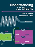
A multimeter (VOM) may be used to measure ac voltage. AC voltage is measured in the same way as direct current (dc) voltage with the following two exceptions:
1. In the measurement of ac voltage, proper polarity does not have to be observed.
2. In the measurement of ac voltage, the ac voltage ranges and scales of the meter must be used.
Figure 2-1 shows the scale of an analog multimeter. The portion used to measure ac voltage is marked. The scales used to measure ac voltage are similar to those used to measure dc voltage.
Measuring AC Voltage with an Oscilloscope
Another way to measure ac voltage is with an oscilloscope. Oscilloscopes, or “scopes,” are used to measure a wide range of frequencies with precision and to examine wave shapes. For electronic servicing, it is necessary to be able to see the voltage waveform while troubleshooting.
When the controls are properly adjusted, an oscilloscope allows various voltage waveforms to be analyzed visually with an image on a screen. This image, called a trace, is usually a line on the screen or cathode ray tube (CRT). A stream of electrons striking the phosphorescent coating on the inside of the screen causes the screen to produce light.
An oscilloscope displays voltage waveforms on two axes, as on a graph. The horizontal axis on the screen is the time axis. The vertical axis is the voltage axis. An ac waveform is displayed on the CRT as shown in Fig. 2-2. For the CRT to display a trace properly, the internal circuits of the scope must be properly adjusted. These adjustments are made with controls on the front of the oscilloscope. Oscilloscopes vary, but most have some of the following controls:

1. Intensity: Controls the brightness of the trace and sometimes is the on-off control.
2. Focus: Adjusts the thickness of the trace so that it is clear and sharp.
3. Vertical position: Adjusts the entire trace up or down.
4. Horizontal position: Adjusts the entire trace left or right
5. Vertical gain: Controls the height of the trace.
6. Horizontal gain: Controls the horizontal size of the trace.
7. Vertical attenuation, or variable volts/centimeter: Acts as a coarse adjustment to reduce the trace vertically.
8. Horizontal sweep, or variable time/centimeter: Controls the speed at which the trace moves across (sweeps) the CRT horizontally. This control determines the number of waveforms displayed on the screen.
9. Synchronization select: Controls how the input to the scope is locked in with the circuitry of the scope.
10. Vertical input: External connections used to apply the input to the vertical circuits of the scope.
11. Horizontal input: External connections used to apply an input to the horizontal circuits of the scope.
The following procedure is used to adjust the controls of an oscilloscope to measure ac voltage. The names of some of the controls vary on different types of oscilloscopes.
1. Turn on the oscilloscope and adjust the intensity and focus controls until a bright, narrow, straight-line trace appears on the screen. Use the horizontal position and vertical position controls to position the trace in the center of the screen. Adjust the horizontal gain and variable time/centimeter until the trace extends from the left side of the screen to the right side of the screen. This allows display of the entire waveform.
2. Connect the proper test probes into the vertical input connections of the oscilloscope.
3. Measure the ac voltage.
4. After a waveform is displayed, adjust the vertical attenuation (volts/centimeter) and vertical gain controls until the height of the trace equals about 2 inches or 4 cm. Most scopes have scales that are marked in centimeters (cm). Adjust the vernier or stability control until the trace becomes stable. One ac waveform or more should appear on the screen of the scope.
Oscilloscope Operation
An oscilloscope is an instrument designed to measure time-varying voltage and current values graphically. This method of measurement allows the operator actually to see voltage and current signal traces rather than viewing the results on a deflection meter or a digital display instrument. In making measurements of this type, the oscilloscope takes very little energy away from the circuit being analyzed. It also responds well to irregularly shaped signal voltages, high frequency, and phase relationships. An oscilloscope is used for calibration of instruments, evaluation of the performance of equipment, and troubleshooting.
The primary function of an oscilloscope is to measure time-varying signals and display these signals so that they can be analyzed. As a rule, a user must prepare this instrument for operation before it can be used to make a suitable display. The setup procedure usually is easy, but it is helpful to know something about basic oscilloscope control functions.
An oscilloscope may be viewed as a series of functional blocks connected together to form an operating system. Presentation of the block structure is an organization procedure that allows the system to be viewed as a functional instrument. It is important to understand the specific role of each block in the operational system and the controls and setup procedures needed to make the oscilloscope function.
The fundamental blocks or parts of an oscilloscope connect together and cause it to respond as an operational system. In general terms, the system is composed of a display device, a horizontal sweep section, vertical amplification and sweep, triggering, power supply, and probes. These functional parts are the same for nearly all oscilloscopes. Figure 2-3 shows these parts in a block diagram.

The blocks of a basic oscilloscope are named according to the specific function they achieve in the operation of the instrument. The vertical section, for example, controls the Y axis, or vertical part of the display. The vertical section controls the up or down motion of the electron beam. The horizontal section of the basic instrument controls left-to-right movement of the electron beam. This part of the instrument produces the X axis of the display. The trigger section determines the specific point in time at which horizontal sweep begins. Triggering is achieved by means of switching action. The CRT is ultimately responsible for graphic display of the signal, the end result of all parts of the system working together. The power supply develops all the operational voltages needed to energize the circuit components. The probe serves as an external input receptacle for the instrument. The combined actions of these functions are needed to make the oscilloscope operational.
CRT
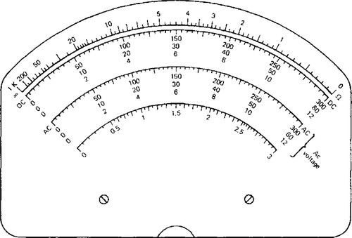
The CRT is responsible for the display function of an oscilloscope. Structurally the CRT is a long, evacuated glass tube in which electrons produced at the neck end of the device cause an image to appear on a glass surface in the display area. Electrons are produced, accelerated, and focused in the rear assembly of the tube. This part of the tube is called the electron gun, or simply the gun. Horizontal and vertical deflection plates are located near the neck area. The electron beam passes through these plates as it moves toward the display area. The large-diameter end of the tube is the display, or viewing, area. The inside glass face of the viewing area is coated with a phosphorescent material. When the high-velocity electron beam strikes this material, it produces a characteristic glow. The CRT changes an invisible electron beam into light energy that is displayed on a glass surface.
Figure 2-4 shows the construction details of a CRT. Figure 2-5 illustrates the operation of the electron gun assembly in the neck of the CRT. A beam of electrons is produced by the cathode of the tube when it is heated by means of application of a filament voltage. Electrons emitted from the cathode are initially attracted by the positive potential of anode 1. The quantity of electrons passing toward anode 1 is determined by the amount of negative bias voltage applied to the control grid. Anode 2 is operated at a higher positive potential than anode 1 to accelerate the electron beam further toward the screen of the CRT. High voltage in the display area of the tube serves as the final attracting force for the electron beam. As it strikes the phosphorescent screen, light is produced.
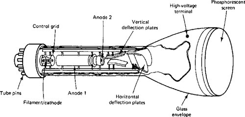
Control of the electron beam is achieved by means of a number of different processes. The quantity of electrons that reach the display area of the CRT determines brightness or intensity level. The intensity control, usually connected to the grid, determines the negative voltage value of the grid. The grid is a small, cylinder-like structure; the end nearest the cathode is open and the other end has a small aperture. The number of electrons forced to pass through the aperture depends on the amount of negative voltage on the grid. High negative voltage repels large numbers of electrons and reduces the level of intensity. Reduced negative voltage increases the quantity of electrons that reach the display area and increases intensity. The intensity control usually is located on the front panel of the oscilloscope.
The sharpness of the display image or trace is determined with the focus control. In a CRT, focus is controlled electrostatically. Electrons emitted from the cathode have a natural tendency to separate, or spread apart, as they move toward the face of the CRT. Each electron, because it has a negative charge, is repelled by its neighboring electrons. This action would normally cause the trace to appear as a large fuzzy ball on the face of the CRT. To alter this condition, focus is achieved by means of altering the difference in the positive voltage between anodes 1 and 2. As a rule, anode 1 is varied and anode 2 remains at a fixed value. Variations in positive voltage cause the trajectory angle of the electron beam to change by means of altering the shape of the electrostatic field. As a result of this adjustment, one can alter the point of convergence of the electron beam by changing a voltage value within the tube. The focus control usually is located on the front panel of the oscilloscope. In most oscilloscopes the focus and intensity control adjustments are interrelated. Adjustment of one control usually necessitates adjustment of the other control.
Deflection
The position of an electron beam in the display area of a CRT is controlled by two sets of deflection plates. These plates are housed in the neck of the CRT and are located between the electron gun and the display area. Figure 2-5 shows the position of these deflection plates near the center of the CRT. The set of plates closest to the gun assembly controls vertical deflection. The second set of plates controls horizontal deflection. The combined effect of these two sets of plates causes the electron beam to have both vertical and horizontal deflection at the same time.
Electron beam deflection of a CRT is accomplished by means of electrostatic charge energy. This energy is produced by means of applying voltages of the correct polarity to the deflection plates. Vertical deflection voltages normally are derived from an external source of energy. This generally represents the signal being viewed on the face of the CRT. Horizontal sweep voltages are developed internally by a time-based generator. Most oscilloscopes have optional circuitry that allows the horizontal sweep signal to be developed externally and applied to the deflection plates. External sweep is selected with a switch.
An end view of a CRT observed from the display area is shown in Fig. 2-6. This representation shows the location of the vertical and horizontal deflection plates with respect to the electron beam. If no voltage is applied to the deflection plates, the electron beam positions itself in the center of the display area. To demonstrate how deflection is achieved, we examine how the electron beam responds when voltage is applied to the deflection plates. We describe the response when voltage is applied to only one set of plates and discuss the response of the electron beam when sweep voltage is applied to both sets of plates at the same time.
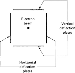
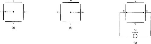
Figure 2-7 shows electron-beam response when voltage is applied only to the vertical deflection plates. If the top vertical plate is made positive and the bottom plate negative, the electron beam is attracted by the top plate and repelled by the bottom plate (Fig. 2-7a). Reversing this polarity causes the beam to move toward the bottom of the CRT (Fig. 2-7b). AC voltage applied to the two plates (Fig. 2-7c) causes the electron beam to sweep from top to bottom according to the applied frequency. High-frequency ac causes the electron beam to appear as a solid vertical line. Low-frequency ac causes a slow-moving dot to be produced by the electron beam. The resulting dot produced by the electron beam moves slowly between the top and bottom of the CRT. The amount of voltage applied determines the length of the vertical sweep pattern.

Figure 2-8 shows the electron-beam response when voltage is applied only to the horizontal deflection plates. In Fig. 2-8a the left horizontal plate is positive, and the right plate is negative. This causes the electron beam to be deflected to the left. Figure 2-8b shows the response of the electron beam when the voltage polarity is reversed. The beam is deflected to the right by this polarity. Figure 2-8c shows the response when ac is applied. In this case, the electron beam sweeps back and forth, producing a horizontal line. The frequency of the applied ac determines the sweep rate.
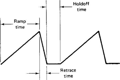
Internally generated horizontal sweep signals generally have a sawtooth shape. This signal, shown in Fig. 2-9, has a linear rise time and a rapid fall time. The rising portion of the wave is called the ramp, and the falling part of the wave is called the retrace. The time or space after retrace is called the holdoff area. The ramp portion of the wave causes sweep from left to right, and retrace causes return of the electron beam to the left side of the display. The holdoff part of the wave determines how long the trace must wait between trigger pulses. The frequency of the sawtooth wave is determined by the sweep rate of the internal horizontal time-base generator.
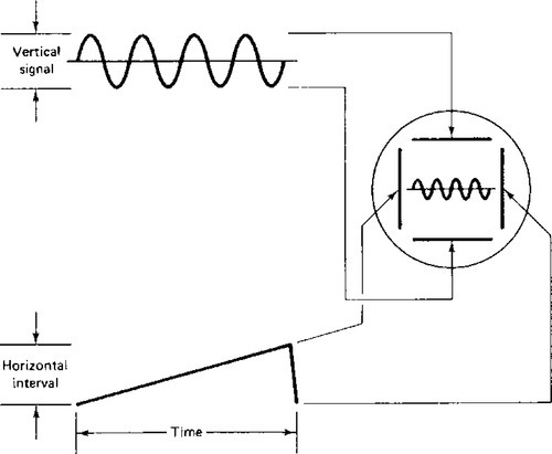
When they are applied simultaneously to the horizontal and vertical deflection plates, sweep signals cause a specific pattern to appear on the face of the CRT. Assume now that an unknown sine wave is to be viewed on the oscilloscope. This wave is supplied to the vertical input for application to the deflection plates. An oscilloscope usually is set up for internal horizontal sweep-signal generation. A sawtooth wave is generated by the time-base generator and applied to the horizontal deflection plates. Figure 2-10 shows the display pattern that appears on the CRT as a result of the applied signals. The beam sweeps from left to right according to the horizontal signal. In the same time frame, the vertical signal causes the electron beam to be deflected up and down according to its voltage value. At any specific point in time, the position of the electron beam is determined by the combined forces of the vertical and horizontal deflection voltage values. These forces cause the sine wave of the vertical input signal to be produced on the CRT. The resulting display is four complete sine waves.
Changing the time period of the horizontal sweep voltage alters the display on the CRT. In Fig. 2-11 the horizontal sweep frequency has been doubled without a change in the vertical input signal. In this case, doubling the horizontal frequency causes the time base to be halved. Time is a function of frequency and is expressed as T = 1/f. When the horizontal sweep is reduced to half its previous value, fewer sine waves are displayed on the CRT. This means that the frequency of the horizontal time-base generator determines the scale of the time axis. The scale or operational range of the time-base generator is controlled by a switch on the front panel of the oscilloscope. This switch is calibrated in units of time per division. Typical ranges are seconds/centimeter (s/cm), milliseconds/centimeter (ms/cm), or microseconds/centimeter (H.s/cm). Specific values in an operating range might be 0.5, 0.2, 0.1 s/division; 50, 20, 10, 5, 2, 1, 0.5, 0.2, 0.1 ms/division; or 50, 20, 10, 5, 2, 1, 0.5, 0.2, 0.1, .05 μs/division.

Triggering and Synchronization
To produce a steady waveform on the face of the CRT, an oscilloscope must repeat the same trace path. For this to be achieved, the displayed signal must always begin its trace at the same point on the wave. Another way of describing this function is to say that the start of the sawtooth voltage must be synchronized with a specific point on the displayed signal. Synchronization of the vertical and horizontal signals is a function of the trigger system.
Figure 2-12 shows signals that are applied to the vertical and horizontal deflection systems and the resulting display produced by an oscilloscope. The top display is the waveform supplied to the vertical deflection system. The middle waveform is produced by the time-base generator and applied to the horizontal deflection system. The bottom trace is the resulting waveform displayed on the CRT. The time-base signal starts its sweep at point a of the sine wave. When the time-base signal completes one trace period, it drops back to its initial voltage value and waits for the next sine wave to return to its beginning point before starting the next trace. This is indicated as point a on the display. Because the resulting image is of a periodic nature and the time base is synchronized to produce exactly the same portion of the signal on each trace, the display image appears to be a stationary sine wave. If the applied signal voltage were to change during the sweep period or if the sweep began at a random point on the input signal voltage, the resulting image would be different for each trace period. This would make the display unsteady or appear to be in a continuous state of motion.
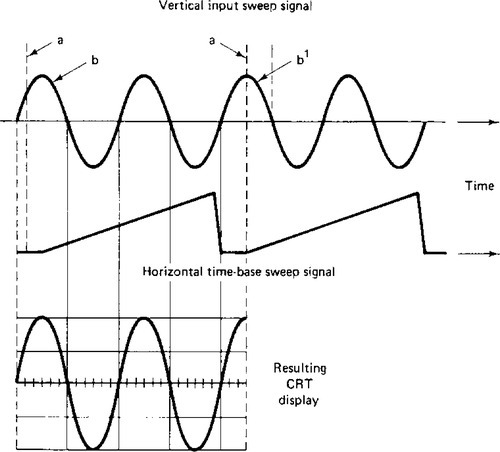
Two controls on an oscilloscope allow the operator to select the point on the display signal where sweep begins. The trigger-level control sets the voltage value that causes the sweep to start. This control alters the starting point or beginning of the display. This function usually is achieved by means of a variable control adjustment. The slope control adjusts the polarity of the voltage where sweep begins. On the display in Fig. 2-12, triggering occurs on the positive slope. If the negative slope were used as the trigger point, sweep would occur at both b points. This would cause the vertical part of the trace to start with a downward motion instead of an upward motion. The slope function is achieved by changing a switch. The slope is either positive or negative according to the desires of the operator.
An oscilloscope generally has some additional trigger controls, depending on its design. One of these is described as the triggering mode of operation. Trigger-mode selection is achieved with a switch. If the EXT trigger mode is selected, the oscilloscope is triggered by an external signal. This signal is derived from the circuit under test or from an external generating source that is used as a reference. With external triggering, it would be possible to observe the phase relations of amplifier input and output signals. Selection of the LINE trigger mode allows the time-base generator to be synchronized by the ac line voltage. This allows the oscilloscope to detect the source of unwanted signals. Noise on a waveform can be made stationary when the signal is synchronized with the line voltage.
Selection of the AUTO mode switch places the oscilloscope in the automatic-triggering mode of operation. Triggering in this manner is considered to be the automatic signal-seeking mode of operation. Assume that a trigger pulse starts the sweep signal. This action causes the electron beam to sweep during the ramp time and retrace period until the holdoff period ends. At this point a timer begins to run. If another trigger does not occur before the timer runs out, a pulse is generated automatically. This allows most signals to be displayed automatically because triggering is duplicated by the internal circuitry of the oscilloscope. This mode of operation also allows the operator to trigger on signals with changing voltage amplitudes or shapes without making level-control adjustments. Automatic triggering is probably the most widely used mode of operation for general oscilloscope work.
Power Supply
The power supply of an oscilloscope is primarily responsible for supplying dc and in some cases ac voltage to the active and passive components of the instrument. These voltage values are derived from the ac power line. Typical primary-line voltage is 120 V at 60 Hz. This voltage is applied to a transformer, which steps the voltage up or down according to the needs of the circuit. The voltage values developed by the supply depend on the circuitry of the oscilloscope and the components being used. For the most part, modern oscilloscopes use solid-state devices. Bipolar transistors, junction field-effect transistors (JFETs), and integrated circuit devices are used in the circuits. As a rule, these devices respond to low-voltage dc energy. The CRT of an oscilloscope, however, requires some rather sizable dc voltage values. DC voltages of 100 to 2000 V are needed to energize the electrodes. The anode of the CRT also may necessitate a dc voltage in the range of 5 to 10 kilovolts (kV). This part of the power supply requires some rather unusual circuitry, such as voltage multipliers or a special high-voltage transformer to develop the necessary voltage values.
The high-voltage supply of an oscilloscope is generally described as a generated voltage source. It develops high-voltage ac from a low-voltage dc source. The dc energizes a transistor that responds as an oscillator. High-frequency ac is supplied to the primary winding of the transformer. The transformer of this circuit can be made smaller because of the high-frequency ac.
Oscilloscope Probes
The probe of an oscilloscope is responsible for connecting voltage and current signals to the vertical input terminais without loading or disturbing the circuit under test. To meet these requirements, a variety of probes are available, from simple passive units to sophisticated active probes for special measurement applications. In each case, the probe must not degrade the performance of the oscilloscope, and it should be properly calibrated to ensure measurement accuracy.
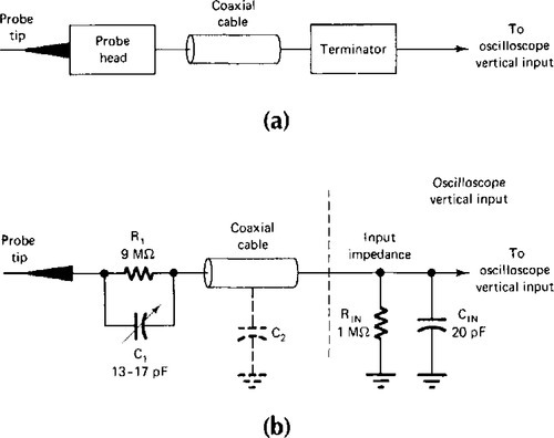
Figure 2-13a shows a general block diagram of an oscilloscope probe. The probe head contains the signal-sensing device. In a passive probe this is achieved with a 10 megohm (MΩ) resistor shunted by a 7 picofarad (pF) capacitor. Active probes have a bipolar transistor, or JFET device, in the probe head. Coaxial cable is used to couple the probe head to the termination circuitry. The termination provides the oscilloscope with the source impedance needed to connect the coaxial cable to the vertical input circuitry.
Passive probes are widely used in most oscilloscope applications. The simplest passive probe is a nonattenuating, or × 1, unit. This type of assembly consists simply of a length of coaxial cable with a probe tip at one end and a cable connector at the other end. Connection is achieved directly through the coaxial cable. Electrically the coaxial cable has some shunting capacitance that must be taken into account. A 50 ohm (Ω) coaxial cable has a shunting capacitance of 30 pF/ft. A 5 ft length of coaxial cable would therefore offer approximately 150 pF of shunt capacitance to the oscilloscope input. This type of probe offers a rather large shunt capacitance to high-frequency ac. As a rule × 1, or direct, probes are used exclusively to measure low-frequency and power-line circuits.
One of the most widely used passive probes is the compensating × 10 attenuating unit (Fig. 2-13b). This probe provides signal attenuation in a ratio of 10:1 over a wide range of frequencies. The probe head has a 9 MΩ resistor shunted by a small variable capacitor. Adjustment of the variable capacitor allows the probe to compensate for impedance changes over a wide range of frequencies. An applied signal should be attenuated by a factor of 10 but still maintain its original shape and phase without distortion. Compensation adjustments allow the probe to couple sample signals to the vertical input without producing distortion and adversely loading down the circuit being evaluated. This adjustment is achieved by means of applying a representative square-wave signal of the frequency being analyzed with the probe. The compensating capacitor is adjusted to produce the best reproduction of the square wave on the CRT. Compensation can be made with a screwdriver adjustment or by means of twisting a barrel capacitor over the probe tip. The structure of the variable capacitor of the probe usually dictates the adjustment procedure.
Oscilloscope Controls
The operating controls of an oscilloscope usually are divided into convenient groups that alter or control a specific instrument function. These include CRT control, vertical deflection, horizontal sweep, triggering, modes of operation, and probes. Each group has a number of unique controls in its makeup. In general, these controls are designed to perform some type of operational procedure. Operational controls are usually placed in a convenient location where they can be easily adjusted.
CRT Display Controls
The CRT display group of oscilloscope controls consists of intensity, focus, trace rotation, and beam finder. These controls are generally located in a position relatively close to the viewing area of the CRT.
Intensity Control
The intensity control of an oscilloscope is used to adjust the brightness level of the display. This is achieved by means of altering the amount of negative voltage going to the control grid of the CRT. Intensity of the electron beam is determined by the quantity or number of electrons that reach the viewing area. When the negative voltage of the grid is reduced in value, a larger number of electrons reach the display area. Increased negative voltage reduces the brightness or intensity of the electron beam. In practice, the intensity control should be adjusted to produce the lowest level of brightness that will allow the display to be viewed effectively. The operational life of the CRT can be prolonged when the intensity of the electron beam is kept to a minimum. Functionally, this control adjusts the brightness level of the trace so that it can be viewed in different ambient light conditions.
Focus
The focus control of an oscilloscope is used primarily to alter the sharpness of the display image. Focus is achieved by means of altering the voltage level of the first anode of the CRT. The potential difference in voltage between first and second anodes of the CRT determines the strength of an electrostatic field. This condition alters the trajectory of the electron beam. A rather large difference in voltage causes the beam to converge into a fine trace near the surface of the viewing area. Focus is simply a voltage adjustment that allows the trace to have fine detail. In most instruments, focus and intensity adjustments are interrelated.
Trace Rotation
The trace rotation control of an oscilloscope is another one of the CRT group of controls included on the front panel of the instrument. Trace rotation allows the user to align the horizontal trace of the display electrically with fixed lines on the graticule (the grid pattern). This control is generally less accessible than the other controls. This is intentional to prevent accidental misalignment of the control. In most oscilloscopes, this adjustment is made with a small screwdriver. Once the adjustment has been made, it generally does not have to be made again unless the instrument is subjected to a stray magnetic field or moved to a different location. In portable instruments this control is very handy because of the different locations in which the instrument is used.
To adjust trace rotation, turn on the instrument and make the necessary adjustments to allow a single horizontal line to be displayed across the center of the display. Position the line so that it is aligned with one of the horizontal lines of the graticule. Adjust the control so that the trace line is parallel to the graticule lines. It may be necessary to adjust the vertical position of the trace again to assure that the two lines are parallel.
Beam Finder
The beam finder of an oscilloscope is a convenience control that allows the user to locate the electron beam when it is off screen. The beam finder is a push-button switch usually located in the CRT group of controls. When this button is depressed, the vertical and horizontal deflection voltages are reduced. This allows the trace to be displayed in the limited space of the face of the CRT. When the operator sees the location of the beam, the vertical and horizontal position controls can be adjusted to center the trace. Some oscilloscopes do not have a beam-finding switch.
Vertical Deflection Controls
The vertical section of an oscilloscope supplies the display part of the instrument with vertical information that ultimately appears on the CRT. The vertical section takes the input signal, amplifies it, and develops a suitable voltage value that deflects the electron beam. The input signal usually is the signal or voltage being analyzed with the oscilloscope. Figure 2-14 is a block diagram of the vertical section of a typical oscilloscope. Controls are attached to different parts of the system. Typical controls are vertical position, input coupling, vertical operating mode, input sensitivity or volts/division selector, and variable volts/division control.

Vertical Position Control
The vertical position control allows the operator to adjust the trace to a desired viewing location. This control adjusts the distribution of voltage between the two deflection plates. If the voltage is equally distributed between the deflection plates, the trace is centered vertical ly. Adjusting the control so that the top plate is more positive than the bottom plate moves the display toward the top of the CRT. Reversing the voltage distribution causes the trace to be positioned near the bottom of the display area.
Vertical Input Coupling
The input coupling function of an oscilloscope is controlled with a switch. This function lets the operator control how the input signal is coupled with the vertical input section of the instrument. In the ac position, the input signal voltage must pass through a capacitor. In the dc position, the input signal is coupled directly to the input of the vertical amplifier. The middle position, or GND, refers to the ground. Placing the switch in this position disconnects the external input signal from the vertical section and grounds the vertical input.
The influence of control on the operation of an oscilloscope can be seen when an appropriate signal is applied to the vertical input. An ac signal adjusts its zero reference point to a value determined by the vertical position control. A dc signal adjusts its reference to a level determined by the voltage value of the applied dc. The ground switch position selects the chassis ground as a reference operating point.
Volts/Division
The volts/division or vertical sensitivity of an oscilloscope is controlled with a rotary switch. This control allows the instrument to extend its range of operation so that signals of a few millivolts to several volts can be displayed on the CRT. Using the volts/division switch also changes the scale factor of the display screen. Each position setting of the switch has a number value that represents the scale factor. The 10 position means that each major vertical division represents 10 V. Other position settings cause a corresponding volts/division function to be established.
All these marked values depend on the variable control being set to the calibrate position. The total amount of vertical sweep or deflection is based on the peak-to-peak voltage of the ac signal being displayed. The probe of an oscilloscope also may have some influence on the amount of vertical sweep produced by the instrument. A × 1 probe provides a direct reading of the volts/division ranges, whereas a 10 probe scales down the input by a factor of 10. The probe and volts/division switch setting of the instrument determine the range of vertical sweep.
Variable Volts/Division Control
Most oscilloscopes have a variable volts/division control that can be used to change the volts/division range setting by a factor of × 2 or more. This control is used to make quick amplitude comparisons of signals. It changes the range of the volts/division setting. In most instruments this control has a notch or position setting where calibration is actuated. The amplitude of the display is reduced or increased with this adjustment. For most oscilloscope applications, the variable control should remain in the calibrate position.
Vertical Operating Mode
The vertical operating mode of an oscilloscope is an operational control for instruments that have two vertical channels. Some oscilloscopes have a duplicate set of vertical controls for each channel. Two independent traces can be displayed on the CRT at the same time. The vertical operating mode is usually a switch function that allows the operator to select a desired channel or a combination of channel options.
The vertical mode switch of a channel selects channel 1, channel 2, or both. The mode switch of a channel often has ADD, ALTERNATE, and CHOP modes of operation. For example, if the channel 1 mode switch is in the BOTH position and the channel 2 switch is in the alternate, or ALT, position, you can adjust the position controls so that the trace of channel 1 is at the top and the trace of channel 2 is near the bottom. If an ac signal is applied to each channel, the volts/division switch of each channel may be adjusted to produce a display of suitable size. The mode switch in the ADD position adds the two traces. The CHOP and ALT mode switches are used to observe two signals at any sweep speed. The alternate mode displays one channel and then the other in an alternate sequence. At high sweep rates, this type of display is very desirable. At slow sweep rates there is a noticeable alternating effect in the two displays. The CHOP mode breaks the two traces into small segments and switches between the two traces very quickly. This is generally noticeable when 60 Hz signals are displayed on the instrument.
Horizontal Sweep Controls
For an oscilloscope to make a display on the face of a CRT, it needs both vertical and horizontal sweeps to deflect the electron beam. Horizontal sweep is normally provided by an internal generator, which produces a sawtooth-shaped waveform. The rising part of this waveform is called the ramp, or trace, period, and the falling part is called the retrace interval. The trace period causes beam deflection from left to right. Retrace causes the beam to return to the left in preparation for the next trace period. The horizontal sweep rate of an oscilloscope is operator controlled, which allows it to display different frequencies.
Figure 2-15 is a block diagram of the horizontal sweep circuitry of an oscilloscope. The circuitry of an oscilloscope is divided into two sections. The generator is responsible for sweep- signal development. The amplifier increases the amplitude of the signal so that it will drive the deflection plates. Controls of this section are attached to the part of the circuit that has the greatest influence on its operation.
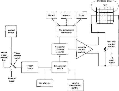
The horizontal sweep of an oscilloscope has a variety of different controls that regulate its operation. These include horizontal position, operational mode, seconds/division, variable sweep, and magnification. These controls are generally grouped together in a special area of the control panel.
Horizontal Position Control
The horizontal position control is designed to change the location of the horizontal trace on the face of the CRT. This adjustment is made by means of shifting the distribution of voltage to the horizontal deflection plates. The trace shifts in the direction of the deflection plate with the highest positive voltage value. As a rule, the horizontal trace should be positioned in the center of the viewing area. The position control should cause the trace to shift from right to left according to the setting of the control. If a dual-channel oscilloscope is used, the position control alters both channels in the same manner.
Horizontal Operating Mode
The horizontal operating mode is an optional function that depends on the degree of sophistication of the oscilloscope. Single time-base oscilloscopes usually have only one mode of operation. Some oscilloscopes are equipped with normal, intensified, and delayed sweep. As a rule, the instrument is used in the normal mode of operation for most applications. In this mode, the horizontal time base responds as an energy source for the horizontal sweep system.
The intensified mode of operation allows the operator to alter the electron beam with a signal voltage that causes its intensity to vary according to an external signal. This mode of operation allows some rather unusual tests to be performed with the oscilloscope. The electron beam of the CRT of a television receiver is intensity modulated to produce light variations in the display.
Delayed sweep allows the instrument to add a precise amount of time between the trigger point and the beginning of the sweep period. With delayed sweep the operator may choose to trigger the trace anywhere along the displayed waveform. The delay time is used to control the start or beginning of the waveform being displayed. For normal measurement applications, the mode switch is placed in the no-delay mode of operation.
Horizontal Time-Base Control
The horizontal time base of an oscilloscope is used to generate a sawtooth wave that deflects the trace horizontally. This action is achieved with a switch that controls the sweep rate of the time-base generator. The switch positions are identified in time/division values. Three ranges of sweep are generally included in an oscilloscope, seconds/division, milliseconds/division, and microseconds/division. A number of discrete values are included in each of these ranges.
The function of this switch is to select the sweep frequency of the horizontal time base. When the frequency of the time base coincides with the frequency of the signal being applied to the vertical input, a suitable display is produced. If the time-base rate is greater or less than the frequency of the observed signal, an unintelligible signal is displayed. The frequency of the time-base generator must be adjusted to a reasonable approximation of the observed signal frequency to produce a meaningful display. Operation of this control is simply a matter of selecting an appropriate sweep range to produce a usable display.
Variable Time/Division Control
The switch positions of the time/division control are designed to provide calibrated time- base values. Sometimes there is a need for variable control of the time base. The variable time/division control allows the operator to adjust the time base. This control is located at the center of the time/division switch. The extreme clockwise position usually places the variable control in the calibrate position. When the control is out of the clockwise position, its variable condition is in effect. This control is left in the calibrate position for most measurement applications.
Horizontal Magnification
Most oscilloscopes offer some means of horizontally magnifying the waveforms that appear on the screen. Magnification is achieved by means of multiplying the time base by a fixed factor. A factor of 10 is typical. This is sometimes achieved by means of pulling out the variable time/division control. This action changes the time-base components by a factor of 10. A 0.05 μs signal can be extended to a 5 nanosecond (ns) signal by engaging the magnification switch. Magnification is very useful for analyzing specific parts of a signal.
Triggering Control
The time-base generator of the horizontal sweep system is considered to be free running. The frequency of the generated sawtooth waveform is based on the RC time constant of circuit components. For this signal to be displayed, there must be some form of synchronization. The horizontal sweep signal must be in step with the vertical signal. The triggering function of an oscilloscope is responsible for selecting a synchronizing signal and applying it to the horizontal sweep generator. Most oscilloscopes are equipped with internal, line, and external triggering capabilities. The trigger system simply tells the oscilloscope which trigger source to use, according to its switch selection. The trigger is adjusted with the slope and level controls to recognize a particular voltage level and polarity. Typical controls of a trigger system are level, slope, variable holdoff, source selection, trigger mode, and coupling.
Variable Holdoff Control
Not every triggering event can be accepted as a trigger pulse for the time-base generator. The trigger system does not recognize triggering during the trace time, the retrace period, or the short time that follows retrace, called the holdoff time. The holdoff period does, however, provide additional time after the retrace period to produce stability. In some applications, the holdoff time may not be long enough to provide good stability of the display. The variable holdoff control allows adjustment of the holdoff time. Changing the holdoff time makes it possible for the instrument to accommodate a trigger point that will appear at the same position on the wave for each repetition of the signal.
Trigger-Operating Modes
The trigger-operating mode of an oscilloscope is used to select different triggering methods for the time-base generator. For example, the MODE switch may have three positions—automatic, normal, and TV field. The normal trigger mode is the most useful. It accommodates the widest range of signals. This mode of operation does not allow a trace to be displayed on the CRT unless the time-base generator is triggered.
In the automatic mode a trigger pulse starts the trace, retrace, and holdoff sequence. At the completion of the sequence, a timer begins its operation. If another trigger pulse does not occur before the timer runs out, a pulse is generated to trigger the next sweep sequence. The automatic mode of triggering is considered to be the signal-seeking mode of operation. This means that for most measuring applications, the automatic mode matches the trigger level to the trigger-signal value. Trigger levels in the automatic mode do not require a value setting outside the signal range. This mode also lets the time-base generator trigger on signals that have changing amplitudes or waveshapes without making level adjustments.
When the trigger-operating mode switch is placed in the TV field position, the oscilloscope becomes useful in television-signal analysis. In this operating mode, the time-base generator triggers on TV fields at 100 μs/division and TV lines at 50 μs/division. This allows the instrument to display video signals, horizontal frequency, vertical, and color-burst signals with good synchronization.
Trigger-Signal Sources
The trigger-signal source of an oscilloscope is divided into three groups. These are described as internal, line, and external. The trigger source of an oscilloscope does not effectively alter operation of the trigger circuit. An internal trigger signal, however, means that the signal being displayed by the CRT also is used to trigger the time-base generator. The triggering source and its switching procedure vary a great deal among different oscilloscope makes and models.
The internal triggering source is enabled when a switch is placed in the INT position. In this position triggering can be from either the vertical channel or the vertical mode of operation. Triggering is determined by the vertical signal. In the VERT MODE position, the trigger source is selected for any of the vertical combinations such as channel A + B, A – B, chopped, A only, or B only. In a sense, this trigger-mode selection procedure is considered to be an automatic internal source-selection procedure.
The LINE source of triggering allows an alternative to the internal triggering source derived from the vertical input signal. Line triggering is very useful for analyzing signals that derive their energy from the ac power source. Line triggering is enabled by means of placing the source switch in the LINE position. This selects the trigger signal from a sample of the ac power line.
An alternative to internal triggering is external triggering. This triggering source comes from an externally supplied signal. External triggering usually gives the operator greater control over the display. To use this triggering source, the operator places the selector switch in the EXT position. The trigger signal must be supplied to the instrument from an outside source. External triggering is useful for analyzing digital signals. An operator might want to look at a long train of very similar pulses while triggering with a signal derived from a clock or another part of the circuit. The external trigger signal also can be used as a reference source in phase analysis of amplifier circuits.
Trigger Coupling
When an external trigger source is applied to an oscilloscope, it generally has signal coupling. The external trigger-coupling circuit can be dc, dc with attenuation, or ac. The dc coupling circuit allows application of both ac and dc signals to the external trigger source. The dc with attenuation input is used to accommodate signals with voltage values greater than those needed for normal signal input. This external trigger-coupling circuit divides the input by a factor of 10. A 100 V input signal divided by 10 equals 10 V. The ac coupling circuit blocks the dc components of the signal and couples only the ac component.
Summary
To use an oscilloscope effectively, the operator must understand the operating controls. These controls set up the instrument for measuring applications.
Self-Examination
Match the oscilloscope control with the proper function. If the control on your scope has a different name, place it in parentheses beside the control name listed.
| _____ 1. Intensity | A. Selects horizontal sweep frequency |
| _____ 2. Focus | B. Provides up and down adjustment of beam |
| _____ 3. Vertical position | C. Determines amplitude of horizontal deflection |
| _____ 4 Horizontal position | D. Controls size of electron beam |
| _____ 5 Vertical gain | E. Provides left and right adjustment of beam |
| _____ 6. Horizontal gain | F. Controls brightness of beam |
| _____ 7. Vertical attenuation | G. Eliminates vertical shift of display |
| _____ 8. Sweep select | H. Connects voltages to the horizontal amplifier |
| _____ 9. Horizontal sweep | I. Determines frequency of the sawtooth sweep |
| _____ 10. Synchronization select | J. Determines amplitude of vertical deflection |
| _____ 11 Horizontal input | K. Reduces vertical input amplitude |
| _____ 12. Vertical input | L. Connects external signals to vertical amplifier |
| M. Determines amount of voltage used to synchronize sweep oscillator | |
| N. Selects type of synchronization desired | |
| O. Balances dc output | |
| P. Sweeps at line frequency |
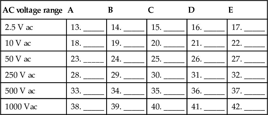
Refer to Fig. 2-16 and determine each of the ac voltage values that correspond to the pointer location.

| AC voltage range | A | B | C | D | E |
| 2.5 V ac | 13. _____ | 14. _____ | 15. _____ | 16. _____ | 17. _____ |
| 10 V ac | 18. _____ | 19. _____ | 20. _____ | 21. _____ | 22. _____ |
| 50 V ac | 23. _____ | 24. _____ | 25. _____ | 26. _____ | 27. _____ |
| 250 V ac | 28. _____ | 29. _____ | 30. _____ | 31. _____ | 32. _____ |
| 500 V ac | 33. _____ | 34. _____ | 35. _____ | 36. _____ | 37. _____ |
| 1000 Vac | 38. _____ | 39. _____ | 40. _____ | 41. _____ | 42. _____ |
Answers
Experimental Activities for AC Electronics
The experimental activities that follow emphasize the practical applications of electronics. They parallel the content of each of the units in this book. The expense of the equipment is kept to a minimum. A few activities require no lab equipment. Each experimental activity is organized in the following way.
A few introductory paragraphs containing an overview of the activity, practical applications, the purpose of the activity, and suggested observations that should be made.
| OBJECTIVE | Expected learning to take place through the experiment. |
| EQUIPMENT | Equipment and materials necessary to perform the experiment. |
| PROCEDURE | Logical, step-by-step sequence for completing the learning activity. Maximum use is made of charts and tables that aid in the recording of data. |
| ANALYSIS | Specific questions and problems that supplement the experimental activity. |
The experimental material is presented in a single-concept approach. Activities organized in this way require only a short time to assemble and make the necessary measurements to facilitate learning.
In this book several experimental activities are used to reinforce the text material. These activities provide a different direction for the learning process. As a rule, the activity is experimentally based. This involves some manipulative activity, or hands-on operation. The activities deal with circuit construction, testing operations, calculations, instrument use, and identification and use of components. Through this approach you will become more familiar with electronic components and their use in a specific circuit application.
Tools and Equipment
A variety of tools and components are needed to perform the experimental activities in this course. These may be obtained from electronics supply houses, mail-order supply houses, and educational vendors. A listing of these sources appears in appendix C.
Important Information
At this time you may want to turn to the back of the book and review the following information:
Appendix A: Electronics Symbols
Appendix D: Soldering Techniques
The information in these sections will help you perform the experimental activities in this book.
Lab Activity Troubleshooting and Testing
The lab activities included in this book provide an opportunity to practice troubleshooting and testing for electronic circuits, devices, and systems. This section is a comprehensive list of troubleshooting and testing procedures that may be accomplished while performing each lab activity. Emphasis should be placed on understanding circuit operation and understanding proper use of test equipment. A technician who understands how the circuit, device, or system functions and knows how to use test equipment will find troubleshooting and testing relatively easy. This is true even for the simplest type of electronic circuit.
Competencies for Troubleshooting and Testing
Specific competencies should be developed during completion of this book. Upon completion of the activities presented in this book, you should be able to do the following.
Objectives
1. Outline basic troubleshooting procedures for locating specific trouble with devices and equipment.
2. Find the parts or circuits that are defective by using a “common sense” approach.
3. Test devices and circuits of electronic equipment using correct procedures.
Competency List
Unit 2: Measuring AC
Experiment 2-1—Measuring AC Voltage
1. Construct a simple ac circuit.
2. Recognize the characteristics of ac circuits.
3. Use a multimeter to measure ac voltage.
4. Compare dc voltage to ac RMS voltage by making voltage measurements.
5. Draw ac voltage waveforms.
6. Convert ac voltage values from a given unit to another including effective (RMS), peak, peak-to-peak, and average values.
7. Convert ac frequency to period (time) and vice versa.
Experiment 2-2—Measuring AC with an Oscilloscope
1. Become familiar with the controls of an oscilloscope.
2. Describe how the adjustment of each oscilloscope control affects the display on the screen of an oscilloscope.
3. Use a signal generator or function generator as an ac voltage source.
Unit 3: Resistance, Inductance, and Capacitance in AC Circuits
Experiment 3-1—Inductance and Inductive Reactance
1. Recognize the effects of ac on the inductive reactance of a coil.
2. Make measurements for an inductive ac circuit with a multimeter.
3. Determine the inductive reactance of a coil by making measurements with a multimeter.
4. Recognize the rating of an inductor (in henrys).
Experiment 3-2—Capacitance and Capacitive Reactance
1. Recognize the effects of ac on the capacitive reactance of a capacitor.
2. Make measurements for a capacitive ac circuit with a multimeter.
3. Determine the capacitive reactance of a capacitor by making measurements with a multimeter.
4. Recognize the working voltage (WVdc) and capacitance (μF or μμF) ratings of capacitors.
Experiment 3-3—Series RL Circuits
1. Recognize the characteristics of a series RL circuit.
2. Measure voltage and current values of a series RL circuit with a multimeter.
3. Compare measured and calculated values of voltage and current of a series RL circuit.
4. Calculate phase angle, impedance, and power factor of a series RL circuit by making measurements with a multimeter.
Experiment 3-4—Series RC Circuits
1. Recognize the characteristics of a series RC circuit.
2. Measure voltage and current values of a series RC circuit with a multimeter.
3. Compare measured and calculated values of voltage and current of a series RC circuit.
4. Calculate phase angle, impedance, and power factor of a series RC circuit by making measurements.
Experiment 3-5—Series RLC Circuits
1. Recognize the characteristics of a series RLC circuit.
2. Measure voltage and current values of a series RLC circuit with a multimeter.
3. Compare measured and calculated values of voltage and current of a series RLC circuit.
4. Calculate phase angle, impedance, and power factor of a series RLC circuit by making measurements.
Experiment 3-6—Parallel RL Circuits
1. Recognize the characteristics of a parallel RL circuit.
2. Measure voltage and current values of a parallel RL circuit with a multimeter.
3. Compare measured and calculated values of voltage and current of a parallel RL circuit.
4. Calculate phase angle, power factor, true power, apparent power, reactive power (VAR), admittance, conductance, susceptance, and impedance of a parallel RL circuit by making measurements.
Experiment 3-7—Parallel RC Circuits
1. Recognize the characteristics of a parallel RC circuit.
2. Measure voltage and current values of a parallel RC circuit with a multimeter.
3. Compare measured and calculated values of voltage and current of a parallel RC circuit.
4. Calculate phase angle, power factor, true power, apparent power, reactive power (VAR), admittance, conductance, susceptance, and impedance of a parallel RC circuit by making measurements.
Unit 4: Transformers
Experiment 4-1—Transformer Analysis
1. Determine the voltage ratio and current ratio of a transformer by making measurements with a multimeter.
2. Sketch a schematic of a transformer.
3. Make resistance measurements on the primary and secondary windings of a transformer.
Unit 5: Frequency-sensitive AC Circuits
Experiment 5-1—Low-pass Filter Circuits
1. Calculate the theoretical frequency response for a low-pass filter circuit.
2. Make measurements with an oscilloscope or multimeter to plot a frequency response curve for a low-pass filter circuit.
3. Use a signal generator or function generator as a variable frequency ac source.
Experiment 5-2—High-pass Filter Circuits
1. Calculate the theoretical frequency response for a high-pass filter circuit.
2. Make measurements with an oscilloscope or multimeter to plot a frequency response curve for a high-pass filter.
Experiment 5-3—Band-pass Filter Circuits
1. Calculate the theoretical frequency response for a band-pass filter circuit.
2. Make measurements with an oscilloscope or multimeter to plot a frequency response curve for a band-pass filter.
Experiment 5-4—Series Resonant Circuits
1. Recognize the characteristics of a series resonant circuit.
2. Measure voltage values of a series resonant circuit with a multimeter or oscilloscope.
3. Determine resonant frequency of a series ac circuit by using a multimeter or oscilloscope.
4. Calculate quality factor and bandwidth of a series resonant circuit by making measurements.
5. Compare measured and calculated values of resonant frequency of a series resonant circuit.
Experiment 5-5—Parallel Resonant Circuits
1. Recognize the characteristics of a parallel resonant circuit.
2. Measure current values of a parallel ac circuit with a multimeter.
3. Determine resonant frequency of a parallel resonant circuit by using a multimeter or oscilloscope.
4. Calculate impedance, quality factor, and bandwidth of a parallel resonant circuit by making measurements.
5. Compare measured and calculated values of resonant frequency of a parallel resonant circuit.
Experiment 2-1
Measuring AC Voltage
Alternating current is the most common form of electric current used in the United States. It is called alternating because it changes its direction periodically. The most frequently used unit of the time associated with ac is the second.
The number of ac cycles per second is known as frequency. Frequency is the number of times in 1 s that the ac moves from zero, reaches a peak in one direction, changes its direction, peaks in the opposite direction, and goes back to zero. These ac cycles per second (cps) are called hertz (Hz). The standard frequency of alternating current and voltage used in the United States is 60 Hz. The period of this standard frequency is 0.0166 s.
Because alternating current, voltage, and power are constantly changing, two types of electric values are used in ac measurement. These are the instantaneous value and the effective value. Instantaneous values are used to describe the value of ac current, voltage, or power at any specified instant. The most common instantaneous value is peak value: the maximum value of voltage, current, or power during any cycle. Effective values are more well known because they are used to describe the amount of voltage, current, and power that can be counted on to produce light, heat, motion, or work of an electric nature. The effective values of ac produce the same amount of work as dc values. Effective values are also called root-mean-square (RMS) values.
Ohm’s laws are used to compute ac values when the opposition to current is resistance only. Instantaneous values of voltage and current must be used to determine instantaneous power. Effective values must be used to determine effective power. The same procedure must be followed when determining voltage or current with a known resistance.
Instantaneous values of voltage, current, and power are converted to effective values, or vice versa, with the mathematical constants 0.707 or 1.41 in the following formulas:
Peak-to-peak values (the distance from peak to peak) of alternating current and voltage are computed with the following formula:
![]()
There is no peak-to-peak value for ac power.
OBJECTIVES
1. To study the characteristics of alternating current (ac).
2. To use a multimeter (VOM) to measure ac voltage.
EQUIPMENT
Multimeter
DC power supply or 6 V battery
AC source: 30 V ac, center tapped with potentiometer adjust
Single Pole Single Throw (SPST) switch
Double Pole Double Throw (DPST) switch
6 V lamp with socket
Resistors: 100 Ω, 220 Ω, 300 Ω.
Connecting wires
PROCEDURE
1. Measure and record the resistance (R) of the filament of the 6 V lamp: R = _______ Ω.
2. Construct the circuit in Fig. 2-1A.

3. Place the switch in position 1 and measure the dc voltage across the 6 V lamp. Record this voltage: ________ V dc.
4. Place the switch in position 2 and disconnect theVOM.
5. Connect a variable ac power supply to the circuit shown in Fig. 2-1B. (Note: Be sure to adjust the ac power supply to zero.) If you do not have a variable ac power supply, variable ac voltage may be obtained as shown from the circuit in Fig. 2-1C.


6. Prepare the VOM to measure ac voltage and connect it across the 6 V lamp.
7. Slowly adjust the variable ac voltage until the VOM reads the same ac voltage as the dc voltage recorded in step 3. Record this voltage: ______ Vac.
8. Slowly change the switch from position 2 to position 1 and back several times. How does this action affect the brightness of the bulb? ________________________________________
9. Using the data from steps 1 and 3, compute the following dc values when the switch is in position 1 :
Current through the lamp: _______ A
Power dissipated by the lamp: _______ W
10. Using the data from steps 1 and 7, compute the following ac values when the DPST switch is in position 2:
Current through the lamp: _______ A
Power dissipated by the lamp: _______ W
11. How did the dc data in step 9 compare with the ac data in step 10? ________________________________________
12. What conclusions can you reach when you compare ac effective values with identical dc values? ________________________________________
13. Disconnect the circuit shown in step 5 and construct the circuit in Fig. 2-1D.
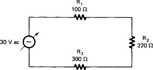
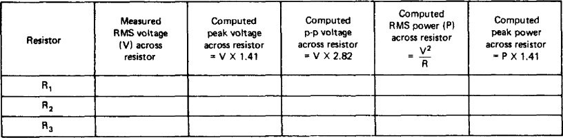
14. Using the VOM to measure ac voltage, complete Fig. 2-1E. Use the proper formulas for the computations.
ANALYSIS
1. Define the following terms:
a. Hertz ____________________
b. Frequency __________________
c. Period __________________
d. Cycle __________________
e. Effective ac values __________________
f. Instantaneous ac values __________________
2. Draw a sine wave in the space to the right. Indicate its four quadrants, positive peak, negative peak, and time base (in degrees).
3. Convert the following effective values to peak and peak-to-peak values.
6 V RMS = _____ V peak; ______ V p-p
4 A RMS = _____ A peak; _____ A p-p
10 V RMS = _____ V peak; _____ V p-p
7 A RMS = _____ A peak; _____ A p-p
4. Convert the following peak values to effective values.
12 W peak = _____ W RMS
100 mA peak = _____ mA RMS
2 mW peak = _____ mW RMS
5. How does the power produced by 10 V dc across 10 Ω compare with the power produced by 10 V ac RMS across the same resistance? ________________________________________
6. Why is a cycle said to consist of 360°? ________________________________________
7. Compute the periods for the following ac frequencies:
1.2 kHz = _______ s
10 kHz = _______ s
1 MHz = ________ s
0.6 MHz = _______ s
60 Hz = _______ s
8. What is the standard frequency of the alternating current used in the United States? ________________________________________
9. What is alternating current? ________________________________________
10. If ac is continually changing its direction, why do the lights in your home not blink on and off? ________________________________________
Experiment 2-2
Measuring AC With an Oscilloscope
An oscilloscope is an electronic instrument that allows various voltage waveforms to be analyzed visually. Somewhat like a television set, it produces an image on a screen when the controls are properly adjusted. The image, called the trace, is usually a line on a screen (CRT). A stream of electrons striking the phosphorous coating on the inside of the screen causes the coating.
An oscilloscope is used to measure frequency and voltage. It can also be used to determine current if used in conjunction with Ohm’s law. The greatest application of an oscilloscope is allowing the operator to see the waveform or signals with which he or she is working.
OBJECTIVES
1. To become familiar with the controls of an oscilloscope.
2. To observe how the adjustments of these controls affect the waveform or trace displayed on the CRT.
3. To use an audio signal generator to supply variable ac voltage to a circuit.
EQUIPMENT
Oscilloscope
Audio signal generator
Resistor: 10 kΩ
Connecting wires
SPST switch
6 V battery
PROCEDURE
1. Turn on the oscilloscope and adjust the intensity and focus controls until a bright, sharp, straight-line trace appears on the screen. Use the horizontal position and vertical position controls to position the trace in the center of the screen. Adjust the horizontal gain until the line trace is long enough to extend from the extreme left to the extreme right side of the screen.
2. Connect the oscilloscope probe into the vertical input jack.
3. Construct the circuit in Fig. 2-2A. Adjust the signal generator to 60 Hz.

4. Connect the oscilloscope probes to points A and B in the circuit of Fig. 2-2A. (Be sure to connect the ground of the oscilloscope to the ground of the signal generator.)
5. Adjust the vertical gain controls until the height of the trace equals about 1 inch. Adjust the horizontal stabilization control until the trace becomes stable. Draw the waveform in the space below.
6. Slowly adjust the vertical gain controls both clockwise and counterclockwise. Describe how this action affects the trace.________________________________________
7. Clockwise adjustment of vertical attenuation control caused the trace to ________________________________________.
Counterclockwise adjustment of the vertical attenuation control caused the trace to ________________________________________.
8. Clockwise adjustment of the vertical gain control caused the trace to ________________________________________.
Counterclockwise adjustment of the vertical gain control caused the trace to ________________________________________.
9. Adjust the horizontal sweep selection and horizontal gain controls both clockwise and counterclockwise. Describe how this action affects the trace.________________________________________
10. Clockwise adjustment of the horizontal sweep selection control caused the trace to ________________________________________.
Counterclockwise adjustment of the horizontal sweep selection control caused the trace to
________________________________________.
11. Clockwise adjustment of the horizontal gain control caused the trace to ________________________________________.
Counterclockwise adjustment of the horizontal gain control caused the trace to ________________________________________.
12. Adjust all of the oscilloscope controls to their maximum counterclockwise positions.
13. Open the SPST switch in the circuit illustrated in Fig. 2-2A. Adjust the signal generator to produce a signal of 1000 Hz.
14. Turn on the oscilloscope and close the switch.
15. Adjust the scope controls until a trace of two sine waves 2 cm in height is produced. Draw these waveforms here:
16. Adjust the scope controls until a trace of four sine waves 1 cm in height is produced. Draw these waveforms here:
17. Slowly adjust the frequency control of the signal generator both clockwise and counterclockwise. Describe what happens to the number of sine waves displayed by the oscilloscope. ________________________________________
18. Open the circuit’s switch and disconnect the signal generator. In its place, connect a 6 V battery.
19. Change the controls of the scope to the dc vertical input. Adjust the vertical attenuation control and the vertical gain control to midrange. Position the trace on the screen as described in step 2.
20. With the scope’s probes connected to points A and B in the circuit, close the SPST switch. Describe what happens to the line trace. Why does it happen? ________________________________________
ANALYSIS
1. What is the most important application of an oscilloscope? ________________________________________
2. Briefly describe the purpose of each of the following controls:
a. Vertical gain ___________
b. Horizontal gain _______________
c. Intensity _______________
d. Focus _____________
e. Vertical position ___________
f. Horizontal position ___________
3. What effect does adjusting the horizontal sweep selection switch have on the trace? ________________________________________
4. What does synchronize mean? ________________________________________
Unit 2 Examination Measuring AC
Instructions: For each of the following questions, circle the answer that most correctly completes the statement.
1. The four values of an ac wave are peak, instantaneous, average, and effective. Which value is normally measured with an ac voltmeter?
b. Average
c. Effective
d. Instantaneous
2. When the volts/division switch is set at 5 V, a sine wave 3 divisions in height is seen on an oscilloscope. What is the peak-to-peak value of the input voltage?
b. 3 V
c. 5 V
d. 15 V
3. A waveform is displayed on an oscilloscope. When the horizontal sweep speed is set at 10 μs/division, and one waveform spans a distance of 4 divisions, what is the frequency of the displayed voltage?
b. 25 kHz
c. 400 kHz
d. 4 MHz
4. What horizontal sweep speed should be used to display one cycle of a 1 MHz signal on an oscilloscope?
b. 0.1 μs/cm
c. 0.5 μs/cm
d. 1 μs/cm
5. If two complete cycles of 5 kHz sine waves are displayed on an oscilloscope, what is the horizontal sweep speed of the oscilloscope?
b. 2.5 ms
c. 5 ms
d. 10 ms
6. What is the time of one cycle of a 1 kHz waveform?
b. 1 s
c. 1 × 10− 3
d. 1 × 10− 6 s
7. What is the frequency of the input signal if three complete cycles are observed spanning 6 divisions on an oscilloscope with a 10 ms horizontal sweep time?
b. 500 Hz
c. 2 kHz
d. 50 kHz
8. What is the vertical height of a 6.3 V RMS signal displayed on an oscilloscope if the 2 V/cm position is selected for vertical gain?
b. 4.41 cm
c. 8.82 cm
d. 17.6 cm
9. What is the purpose of the calibration output on an oscilloscope?
a. Calibrate the vertical (V/division)
b. Calibrate the horizontal (time/division)
c. Calibrate the rise time
d. Calibrate the bandwidth
10. When measuring ac voltage with a VOM
b. The meter must be recalibrated before each measurement.
c. Polarity is not observed.
d. The “dc volts” setting is used to measure RMS values.
True or false: Place either T or F in each blank.
| ______ 11. | An oscilloscope is an instrument that allows its operator to analyze voltage waveforms visually. |
| ______ 12. | The image or waveform displayed by an oscilloscope is sometimes called the trace. |
| ______ 13. | An oscilloscope displays the voltage waveforms on three axes: vertical, horizontal, and time. |
| ______ 14. | The brightness of a waveform displayed by an oscilloscope is controlled with the focus control. |
| ______ 15. | The horizontal gain control of an oscilloscope is used to control the display height of the waveform. |
| ______ 16. | The intensity control is used to adjust the displayed waveform to cause it to become clear and sharp. |
| ______ 17. | The vertical position control is used to adjust the displayed waveform up and down. |
| ______ 18. | The inside of the CRT is coated with potassium hydroxide and glows when struck with the beam of electrons. |
| ______ 19. | The oscilloscope can be used to measure frequency as well as voltage. |
| ______ 20. | The horizontal gain control is used to adjust the waveform to the left or right. |