Chapter 7. Universality Is Everywhere
Most of the complexity we see in the world comes from complicated systems—mammals, microprocessors, the economy, the weather—so it’s natural to assume that a simple system can only do simple things. But in this book, we’ve seen that simple systems can have impressive capabilities: Chapter 6 showed that even a very minimal programming language has enough power to do useful work, and Chapter 5 sketched the design of a universal Turing machine that can read an encoded description of another machine and then simulate its execution.
The existence of the universal Turing machine is extremely significant. Even though any individual Turing machine has a hardcoded rulebook, the universal Turing machine demonstrates that it’s possible to design a device that can adapt to arbitrary tasks by reading instructions from a tape. These instructions are effectively a piece of software that controls the operation of the machine’s hardware, just like in the general-purpose programmable computers we use every day.[53] Finite and pushdown automata are slightly too simple to support this kind of full-blown programmability, but a Turing machine has just enough complexity to make it work.
In this chapter, we’ll take a tour of several simple systems and see that they’re all universal—all capable of simulating a Turing machine, and therefore all capable of executing an arbitrary program provided as input instead of hardcoded into the rules of the system—which suggests that universality is a lot more common than we might expect.
Lambda Calculus
We’ve seen that the lambda calculus is a usable programming language, but we haven’t yet explored whether it’s as powerful as a Turing machine. In fact, the lambda calculus must be at least that powerful, because it turns out to be capable of simulating any Turing machine, including (of course) a universal Turing machine.
Let’s get a taste of how that works by quickly implementing part of a Turing machine—the tape—in the lambda calculus.
Note
As in Chapter 6, we’re going to take the convenient shortcut of representing lambda calculus expressions as Ruby code, as long as that code does nothing except make procs, call procs, and use constants as abbreviations.
It’s a little risky to bring Ruby into play when it’s not the language we’re supposed to be investigating, but in exchange, we get a familiar syntax for expressions and an easy way to evaluate them, and our discoveries will still be valid as long as we stay within the constraints.
A Turing machine tape has four attributes: the list of characters appearing on the left of the tape, the character in the middle of the tape (where the machine’s read/write head is), the list of characters on the right, and the character to be treated as a blank. We can represent those four values as a pair of pairs:
TAPE=->l{->m{->r{->b{PAIR[PAIR[l][m]][PAIR[r][b]]}}}}TAPE_LEFT=->t{LEFT[LEFT[t]]}TAPE_MIDDLE=->t{RIGHT[LEFT[t]]}TAPE_RIGHT=->t{LEFT[RIGHT[t]]}TAPE_BLANK=->t{RIGHT[RIGHT[t]]}
TAPE acts as a constructor that
takes the four tape attributes as arguments and returns a proc
representing a tape, and TAPE_LEFT,
TAPE_MIDDLE, TAPE_RIGHT, and TAPE_BLANK are the accessors that can take one
of those tape representations and pull the corresponding attribute out
again.
Once we have this data structure, we can implement TAPE_WRITE, which takes a tape and a character and returns a new tape with that
character written in the middle position:
TAPE_WRITE=->t{->c{TAPE[TAPE_LEFT[t]][c][TAPE_RIGHT[t]][TAPE_BLANK[t]]}}
We can also define operations to move the tape head. Here’s a
TAPE_MOVE_HEAD_RIGHT proc for moving
the head one square to the right, converted directly from the unrestricted
Ruby implementation of Tape#move_head_right in Simulation:[54]
TAPE_MOVE_HEAD_RIGHT=->t{TAPE[PUSH[TAPE_LEFT[t]][TAPE_MIDDLE[t]]][IF[IS_EMPTY[TAPE_RIGHT[t]]][TAPE_BLANK[t]][FIRST[TAPE_RIGHT[t]]]][IF[IS_EMPTY[TAPE_RIGHT[t]]][EMPTY][REST[TAPE_RIGHT[t]]]][TAPE_BLANK[t]]}
Taken together, these operations give us everything we need to create a tape, read from it, write onto it, and move its head around. For example, we can start with a blank tape and write a sequence of numbers into consecutive squares:
>>current_tape=TAPE[EMPTY][ZERO][EMPTY][ZERO]=> #<Proc (lambda)>>>current_tape=TAPE_WRITE[current_tape][ONE]=> #<Proc (lambda)>>>current_tape=TAPE_MOVE_HEAD_RIGHT[current_tape]=> #<Proc (lambda)>>>current_tape=TAPE_WRITE[current_tape][TWO]=> #<Proc (lambda)>>>current_tape=TAPE_MOVE_HEAD_RIGHT[current_tape]=> #<Proc (lambda)>>>current_tape=TAPE_WRITE[current_tape][THREE]=> #<Proc (lambda)>>>current_tape=TAPE_MOVE_HEAD_RIGHT[current_tape]=> #<Proc (lambda)>>>to_array(TAPE_LEFT[current_tape]).map{|p|to_integer(p)}=> [1, 2, 3]>>to_integer(TAPE_MIDDLE[current_tape])=> 0>>to_array(TAPE_RIGHT[current_tape]).map{|p|to_integer(p)}=> []
We’ll skip over the rest of the details, but it’s not difficult to continue like this,
building proc-based representations of states, configurations, rules, and rulebooks. Once we
have all those pieces, we can write proc-only implementations of DTM#step and DTM#run: STEP simulates a single step of a Turing machine by applying a rulebook to one
configuration to produce another, and RUN simulates a
machine’s full execution by using the Z combinator to repeatedly call STEP until no rule applies or the machine reaches a halting state.
In other words, RUN is a lambda
calculus program that can simulate any Turing machine.[55] It turns out that the reverse is also possible: a Turing
machine can act as an interpreter for the lambda calculus by storing a
representation of a lambda calculus expression on the tape and repeatedly
updating it according to a set of reduction rules, just like the
operational semantics from Semantics.
Note
Since every Turing machine can be simulated by a lambda calculus program, and every lambda calculus program can be simulated by a Turing machine, the two systems are exactly equivalent in power. That’s a surprising result, because Turing machines and lambda calculus programs work in completely different ways and there’s no prior reason to expect them to have identical capabilities.
This means there’s at least one way to simulate the lambda calculus in itself: first implement a Turing machine in the lambda calculus, then use that simulated machine to run a lambda calculus interpreter. This simulation-inside-a-simulation is a very inefficient way of doing things, and we can get the same result more elegantly by designing data structures to represent lambda calculus expressions and then implementing an operational semantics directly, but it does show that the lambda calculus must be universal without having to build anything new. A self-interpreter is the lambda calculus version of the universal Turing machine: even though the underlying interpreter program is fixed, we can make it do any job by supplying a suitable lambda calculus expression as input.
As we’ve seen, the real benefit of a universal system is that it can be programmed to perform different tasks, rather than always being hardcoded to perform a single one. In particular, a universal system can be programmed to simulate any other universal system; a universal Turing machine can evaluate lambda calculus expressions, and a lambda calculus interpreter can simulate the execution of a Turing machine.
Partial Recursive Functions
In much the same way that lambda calculus expressions consist entirely of
creating and calling procs, partial recursive
functions are programs that are constructed from four
fundamental building blocks in different combinations. The first two
building blocks are called zero and
increment, and we can implement them
here as Ruby methods:
defzero0enddefincrement(n)n+1end
These are straightforward methods that return the number zero and add one to a number respectively:
>>zero=> 0>>increment(zero)=> 1>>increment(increment(zero))=> 2
We can use #zero and #increment to define some new methods, albeit
not very interesting ones:
>>deftwoincrement(increment(zero))end=> nil>>two=> 2>>defthreeincrement(two)end=> nil>>three=> 3>>defadd_three(x)increment(increment(increment(x)))end=> nil>>add_three(two)=> 5
The third building block, #recurse, is more complicated:
defrecurse(f,g,*values)*other_values,last_value=valuesiflast_value.zero?send(f,*other_values)elseeasier_last_value=last_value-1easier_values=other_values+[easier_last_value]easier_result=recurse(f,g,*easier_values)send(g,*easier_values,easier_result)endend
#recurse takes two method names
as arguments, f and g, and uses them to perform a recursive
calculation on some input values. The immediate result of a call to
#recurse is computed by delegating to
either f or g depending on what the last input value
is:
If the last input value is zero,
#recursecalls the method named byf, passing the rest of the values as arguments.If the last input value is not zero,
#recursedecrements it, calls itself with the updated input values, and then calls the method named bygwith those same values and the result of the recursive call.
This sounds more complicated than it is; #recurse is
just a template for defining a certain kind of recursive function. For example, we can use it
to define a method called #add that takes two arguments,
x and y, and adds them
together. To build this method with #recurse, we need to
implement two other methods that answer these questions:
Given the value of
x, what is the value ofadd(x, 0)?Given the values of
x,y - 1, andadd(x, y - 1), what is the value ofadd(x, y)?
The first question is easy: adding zero to a number doesn’t change
it, so if we know the value of x, the
value of add(x, 0) will be identical.
We can implement this as a method called #add_zero_to_x that simply returns its
argument:
defadd_zero_to_x(x)xend
The second question is slightly harder, but still simple enough to answer: if we already
have the value of add(x, y - 1), we just need to increment
it to get the value of add(x, y).[56] This means we need a method that increments its third argument (#recurse calls it with x,
y -
            1
, and add(x, y -
1)). Let’s call it #increment_easier_result:
defincrement_easier_result(x,easier_y,easier_result)increment(easier_result)end
Putting these together gives us a definition of #add
built out of #recurse and #increment:
defadd(x,y)recurse(:add_zero_to_x,:increment_easier_result,x,y)end
Note
The same spirit applies here as in Chapter 6: we may only use method
definitions to give convenient names to expressions, not to sneak
recursion into them.[57] If we want to write a recursive method, we have to use
#recurse.
Let’s check that #add does what
it’s supposed to:
>>add(two,three)=> 5
Looks good. We can use the same strategy to implement other familiar
examples, like #multiply…
defmultiply_x_by_zero(x)zeroenddefadd_x_to_easier_result(x,easier_y,easier_result)add(x,easier_result)enddefmultiply(x,y)recurse(:multiply_x_by_zero,:add_x_to_easier_result,x,y)end
…and #decrement…
defeasier_x(easier_x,easier_result)easier_xenddefdecrement(x)recurse(:zero,:easier_x,x)end
…and #subtract:
defsubtract_zero_from_x(x)xenddefdecrement_easier_result(x,easier_y,easier_result)decrement(easier_result)enddefsubtract(x,y)recurse(:subtract_zero_from_x,:decrement_easier_result,x,y)end
These implementations all work as expected:
>>multiply(two,three)=> 6>>defsixmultiply(two,three)end=> nil>>decrement(six)=> 5>>subtract(six,two)=> 4>>subtract(two,six)=> 0
The programs that we can assemble out of #zero,
#increment, and #recurse are called the primitive recursive functions.
All primitive recursive functions are total: regardless of their
inputs, they always halt and return an answer. This is because #recurse is the only legitimate way to define a recursive method, and #recurse always halts: each recursive call makes the last argument
closer to zero, and when it inevitably reaches zero, the recursion will stop.
#zero, #increment,
and #recurse are enough to construct many useful functions,
including all the operations needed to perform a single step of a Turing machine: the contents
of a Turing machine tape can be represented as a large number, and primitive recursive
functions can be used to read the character at the tape head’s current position, write a new
character onto the tape, and move the tape head left or right. However, we can’t simulate the
full execution of an arbitrary Turing machine with primitive recursive functions, because some
Turing machines loop forever, so primitive recursive functions aren’t universal.
To get a truly universal system we have to add a fourth fundamental operation, #minimize:
defminimizen=0n=n+1untilyield(n).zero?nend
#minimize takes a block and calls it repeatedly with a
single numeric argument. For the first call, it provides 0
as the argument, then 1, then 2, and keeps calling the block with larger and larger numbers until it returns
zero.
By adding #minimize to #zero, #increment, and #recurse, we can build many more functions—all the
partial recursive functions—including ones that don’t always halt. For
example, #minimize gives us an easy way to implement
#divide:
defdivide(x,y)minimize{|n|subtract(increment(x),multiply(y,increment(n)))}end
Note
The expression subtract(increment(x),
multiply(y, increment(n))) is designed to return zero for
values of n that make y * (n + 1) greater than x. If we’re trying to divide 13 by 4 (x = 13, y =
4), look at the values of y * (n +
1) as n increases:
| n | x | y * (n + 1) | Is y * (n + 1) greater than x? |
0 | 13 | 4 | no |
1 | 13 | 8 | no |
2 | 13 | 12 | no |
3 | 13 | 16 | yes |
4 | 13 | 20 | yes |
5 | 13 | 24 | yes |
The first value of n that satisfies the condition is
3, so the block we pass to #minimize will return zero for the first time when n reaches 3, and we’ll get 3 as the result of divide(13,
4).
When #divide is called with sensible arguments, it
always returns a result, just like a primitive recursive function:
>>divide(six,two)=> 3>>deftenincrement(multiply(three,three))end=> nil>>ten=> 10>>divide(ten,three)=> 3
But #divide doesn’t have to return an answer, because
#minimize can loop forever. #divide by zero is undefined:
>>divide(six,zero)SystemStackError: stack level too deep
Warning
It’s a little surprising to see a stack overflow here, because the implementation of
#minimize is iterative and doesn’t directly grow the
call stack, but the overflow actually happens during #divide’s call to the recursive #multiply
method. The depth of recursion in the #multiply call is
determined by its second argument, increment(n), and the
value of n becomes very large as the #minimize loop tries to run forever, eventually overflowing the
stack.
With #minimize, it’s possible to fully simulate a
Turing machine by repeatedly calling the primitive recursive function that performs a single
simulation step. The simulation will continue until the machine halts—and if that never
happens, it’ll run forever.
SKI Combinator Calculus
The SKI combinator calculus is a system of rules for manipulating the syntax of expressions,
just like the lambda calculus. Although the lambda calculus is already
very simple, it still has three kinds of expression—variables, functions,
and calls—and we saw in Semantics that
variables make the reduction rules a bit complicated. The SKI calculus is
even simpler, with only two kinds of expression—calls and alphabetic
symbols—and much easier rules. All of its power
comes from the three special symbols S,
K, and I (called combinators),
each of which has its own reduction rule:
Reduce
S[toa][b][c]a[c][b[c]]abcReduce
K[toa][b]aReduce
I[toa]a
For example, here’s one way of reducing the expression I[S][K][S][I[K]]:
I[S][K][S][I[K]] → S[K][S][I[K]] (reduceI[S]toS) → S[K][S][K] (reduceI[K]toK) → K[K][S[K]] (reduceS[K][S][K]toK[K][S[K]]) → K (reduceK[K][S[K]]toK)
Notice that there’s no lambda-calculus-style variable replacement going on here, just symbols being reordered, duplicated, and discarded according to the reduction rules.
It’s easy to implement the abstract syntax of SKI expressions:
classSKISymbol<Struct.new(:name)defto_sname.to_senddefinspectto_sendendclassSKICall<Struct.new(:left,:right)defto_s"#{left}[#{right}]"enddefinspectto_sendendclassSKICombinator<SKISymbolendS,K,I=[:S,:K,:I].map{|name|SKICombinator.new(name)}
Note
Here we’re defining SKICall and
SKISymbol classes to represent calls
and symbols generally, then creating the one-off instances S, K, and
I to represent those particular
symbols that act as combinators.
We could have made S, K, and I direct instances of SKISymbol, but instead, we’ve used instances of a subclass
called SKICombinator. This doesn’t help us right now, but
it’ll make it easier to add methods to all three combinator objects later on.
These classes and objects can be used to build abstract syntax trees of SKI expressions:
>>x=SKISymbol.new(:x)=> x>>expression=SKICall.new(SKICall.new(S,K),SKICall.new(I,x))=> S[K][I[x]]
We can give the SKI calculus a small-step operational semantics by implementing its
reduction rules and applying those rules inside expressions. First, we’ll define a method
called #call on the SKICombinator instances; S, K, and I each get their own
definition of #call that implements their reduction
rule:
# reduce S[a][b][c] toa[c][b[c]]defS.call(a,b,c)SKICall.new(SKICall.new(a,c),SKICall.new(b,c))end# reduce K[a][b] toadefK.call(a,b)aend# reduce I[a] toadefI.call(a)aend
Okay, so this gives us a way to apply the rules of the calculus if we already know what arguments a combinator is being called with…
>>y,z=SKISymbol.new(:y),SKISymbol.new(:z)=> [y, z]>>S.call(x,y,z)=> x[z][y[z]]
…but to use #call with a real SKI expression, we need
to extract a combinator and arguments from it. This is a bit fiddly since an expression is
represented as a binary tree of SKICall objects:
>>expression=SKICall.new(SKICall.new(SKICall.new(S,x),y),z)=> S[x][y][z]>>combinator=expression.left.left.left=> S>>first_argument=expression.left.left.right=> x>>second_argument=expression.left.right=> y>>third_argument=expression.right=> z>>combinator.call(first_argument,second_argument,third_argument)=> x[z][y[z]]
To make this structure easier to handle, we can define the methods
#combinator and #arguments on abstract syntax trees:
classSKISymboldefcombinatorselfenddefarguments[]endendclassSKICalldefcombinatorleft.combinatorenddefargumentsleft.arguments+[right]endend
This gives us an easy way to discover which combinator to call and what arguments to pass to it:
>>expression=> S[x][y][z]>>combinator=expression.combinator=> S>>arguments=expression.arguments=> [x, y, z]>>combinator.call(*arguments)=> x[z][y[z]]
That works fine for S[x][y][z], but there are a couple
of problems in the general case. First, the #combinator
method just returns the leftmost symbol from an expression, but that
symbol isn’t necessarily a combinator:
>>expression=SKICall.new(SKICall.new(x,y),z)=> x[y][z]>>combinator=expression.combinator=> x>>arguments=expression.arguments=> [y, z]>>combinator.call(*arguments)NoMethodError: undefined method `call' for x:SKISymbol
And second, even if the leftmost symbol is a combinator, it isn’t necessarily being called with the right number of arguments:
>>expression=SKICall.new(SKICall.new(S,x),y)=> S[x][y]>>combinator=expression.combinator=> S>>arguments=expression.arguments=> [x, y]>>combinator.call(*arguments)ArgumentError: wrong number of arguments (2 for 3)
To avoid both these problems, we’ll define a #callable?
predicate for checking whether it’s appropriate to use #call with the results of #combinator and
#arguments. A vanilla symbol is never callable, and a
combinator is only callable if the number of arguments is correct:
classSKISymboldefcallable?(*arguments)falseendenddefS.callable?(*arguments)arguments.length==3enddefK.callable?(*arguments)arguments.length==2enddefI.callable?(*arguments)arguments.length==1end
Note
Incidentally, Ruby already has a way to ask a method how many arguments it expects (its arity):
>>defadd(x,y)x+yend=> nil>>add_method=method(:add)=> #<Method: Object#add>>>add_method.arity=> 2
So we could replace S, K, and I’s
separate implementations of #callable? with a shared one:
classSKICombinatordefcallable?(*arguments)arguments.length==method(:call).arityendend
Now we can recognize expressions where the reduction rules directly apply:
>>expression=SKICall.new(SKICall.new(x,y),z)=> x[y][z]>>expression.combinator.callable?(*expression.arguments)=> false>>expression=SKICall.new(SKICall.new(S,x),y)=> S[x][y]>>expression.combinator.callable?(*expression.arguments)=> false>>expression=SKICall.new(SKICall.new(SKICall.new(S,x),y),z)=> S[x][y][z]>>expression.combinator.callable?(*expression.arguments)=> true
We’re finally ready to implement the familiar #reducible? and #reduce methods for SKI expressions:
classSKISymboldefreducible?falseendendclassSKICalldefreducible?left.reducible?||right.reducible?||combinator.callable?(*arguments)enddefreduceifleft.reducible?SKICall.new(left.reduce,right)elsifright.reducible?SKICall.new(left,right.reduce)elsecombinator.call(*arguments)endendend
Note
SKICall#reduce works by
recursively looking for a subexpression that we know how to reduce—the
S combinator being called with three
arguments, for instance—and then applying the appropriate rule with
#call.
And that’s it! We can now evaluate SKI expressions by repeatedly
reducing them until no more reductions are possible. For example, here’s
the expression S[K[S[I]]][K], which
swaps the order of its two arguments, being called with the symbols
x and y:
>>swap=SKICall.new(SKICall.new(S,SKICall.new(K,SKICall.new(S,I))),K)=> S[K[S[I]]][K]>>expression=SKICall.new(SKICall.new(swap,x),y)=> S[K[S[I]]][K][x][y]>>whileexpression.reducible?putsexpressionexpression=expression.reduceend;putsexpressionS[K[S[I]]][K][x][y]K[S[I]][x][K[x]][y]S[I][K[x]][y]I[y][K[x][y]]y[K[x][y]]y[x]=> nil
The SKI calculus can produce surprisingly complex behavior with its three simple rules—so complex, in fact, that it turns out to be universal. We can prove it’s universal by showing how to translate any lambda calculus expression into an SKI expression that does the same thing, effectively using the SKI calculus to give a denotational semantics for the lambda calculus. We already know that the lambda calculus is universal, so if the SKI calculus can completely simulate it, it follows that the SKI calculus is universal too.
At the heart of the translation is a method called #as_a_function_of:
classSKISymboldefas_a_function_of(name)ifself.name==nameIelseSKICall.new(K,self)endendendclassSKICombinatordefas_a_function_of(name)SKICall.new(K,self)endendclassSKICalldefas_a_function_of(name)left_function=left.as_a_function_of(name)right_function=right.as_a_function_of(name)SKICall.new(SKICall.new(S,left_function),right_function)endend
The precise details of how #as_a_function_of works aren’t important, but
roughly speaking, it converts an SKI expression into a new one that turns
back into the original when called with an argument. For example, the
expression S[K][I] gets converted into
S[S[K[S]][K[K]]][K[I]]:
>>original=SKICall.new(SKICall.new(S,K),I)=> S[K][I]>>function=original.as_a_function_of(:x)=> S[S[K[S]][K[K]]][K[I]]>>function.reducible?=> false
When S[S[K[S]][K[K]]][K[I]] is called with an argument,
say, the symbol y, it reduces back to S[K][I]:
>>expression=SKICall.new(function,y)=> S[S[K[S]][K[K]]][K[I]][y]>>whileexpression.reducible?putsexpressionexpression=expression.reduceend;putsexpressionS[S[K[S]][K[K]]][K[I]][y]S[K[S]][K[K]][y][K[I][y]]K[S][y][K[K][y]][K[I][y]]S[K[K][y]][K[I][y]]S[K][K[I][y]]S[K][I]=> nil>>expression==original=> true
The name parameter is only used if the original
expression contains a symbol with that name. In that case, #as_a_function_of produces something more interesting: an expression that, when
called with an argument, reduces to the original expression with that argument in place of the
symbol:
>>original=SKICall.new(SKICall.new(S,x),I)=> S[x][I]>>function=original.as_a_function_of(:x)=> S[S[K[S]][I]][K[I]]>>expression=SKICall.new(function,y)=> S[S[K[S]][I]][K[I]][y]>>whileexpression.reducible?putsexpressionexpression=expression.reduceend;putsexpressionS[S[K[S]][I]][K[I]][y]S[K[S]][I][y][K[I][y]]K[S][y][I[y]][K[I][y]]S[I[y]][K[I][y]]S[y][K[I][y]]S[y][I]=> nil>>expression==original=> false
This is an explicit reimplementation of the way that variables get
replaced inside the body of a lambda calculus function when it’s called.
Essentially, #as_a_function_of gives us
a way to use an SKI expression as the body of a function: it creates a new
expression that behaves just like a function with a particular body and
parameter name, even though the SKI calculus doesn’t have explicit syntax
for functions.
The ability of the SKI calculus to imitate the behavior of functions
makes it straightforward to translate lambda calculus expressions into SKI
expressions. Lambda calculus variables and calls become SKI calculus
symbols and calls, and each lambda calculus function has its body turned
into an SKI calculus “function” with #as_a_function_of:
classLCVariabledefto_skiSKISymbol.new(name)endendclassLCCalldefto_skiSKICall.new(left.to_ski,right.to_ski)endendclassLCFunctiondefto_skibody.to_ski.as_a_function_of(parameter)endend
Let’s check this translation by converting the lambda calculus representation of the number two (see Numbers) into the SKI calculus:
>>two=LambdaCalculusParser.new.parse('-> p { -> x { p[p[x]] } }').to_ast=> -> p { -> x { p[p[x]] } }>>two.to_ski=> S[S[K[S]][S[K[K]][I]]][S[S[K[S]][S[K[K]][I]]][K[I]]]
Does the SKI calculus expression S[S[K[S]][S[K[K]][I]]][S[S[K[S]][S[K[K]][I]]][K[I]]]
do the same thing as the lambda calculus expression -> p { -> x { p[p[x]] } }? Well, it’s
supposed to call its first argument twice on its second argument, so we
can try giving it some arguments to see whether it actually does that,
just like we did in Semantics:
>>inc,zero=SKISymbol.new(:inc),SKISymbol.new(:zero)=> [inc, zero]>>expression=SKICall.new(SKICall.new(two.to_ski,inc),zero)=> S[S[K[S]][S[K[K]][I]]][S[S[K[S]][S[K[K]][I]]][K[I]]][inc][zero]>>whileexpression.reducible?putsexpressionexpression=expression.reduceend;putsexpressionS[S[K[S]][S[K[K]][I]]][S[S[K[S]][S[K[K]][I]]][K[I]]][inc][zero]S[K[S]][S[K[K]][I]][inc][S[S[K[S]][S[K[K]][I]]][K[I]][inc]][zero]K[S][inc][S[K[K]][I][inc]][S[S[K[S]][S[K[K]][I]]][K[I]][inc]][zero]S[S[K[K]][I][inc]][S[S[K[S]][S[K[K]][I]]][K[I]][inc]][zero]S[K[K][inc][I[inc]]][S[S[K[S]][S[K[K]][I]]][K[I]][inc]][zero]S[K[I[inc]]][S[S[K[S]][S[K[K]][I]]][K[I]][inc]][zero]S[K[inc]][S[S[K[S]][S[K[K]][I]]][K[I]][inc]][zero]S[K[inc]][S[K[S]][S[K[K]][I]][inc][K[I][inc]]][zero]S[K[inc]][K[S][inc][S[K[K]][I][inc]][K[I][inc]]][zero]S[K[inc]][S[S[K[K]][I][inc]][K[I][inc]]][zero]S[K[inc]][S[K[K][inc][I[inc]]][K[I][inc]]][zero]S[K[inc]][S[K[I[inc]]][K[I][inc]]][zero]S[K[inc]][S[K[inc]][K[I][inc]]][zero]S[K[inc]][S[K[inc]][I]][zero]K[inc][zero][S[K[inc]][I][zero]]inc[S[K[inc]][I][zero]]inc[K[inc][zero][I[zero]]]inc[inc[I[zero]]]inc[inc[zero]]=> nil
Sure enough, calling the converted expression with symbols named
inc and zero has evaluated to inc[inc[zero]], which is exactly what we wanted.
The same translation works successfully for any other lambda calculus
expression, so the SKI combinator calculus can completely simulate the
lambda calculus, and therefore must be universal.
Note
Although the SKI calculus has three combinators, the I combinator is actually redundant. There are
many expressions containing only S
and K that do the same thing as
I; for instance, look at the behavior
of S[K][K]:
>>identity=SKICall.new(SKICall.new(S,K),K)=> S[K][K]>>expression=SKICall.new(identity,x)=> S[K][K][x]>>whileexpression.reducible?putsexpressionexpression=expression.reduceend;putsexpressionS[K][K][x]K[x][K[x]]x=> nil
So S[K][K] has the same behavior as I, and in fact, that’s true for any SKI expression of the form
S[K][. The whatever]I combinator is syntactic sugar that we can live without; just
the two combinators S and K are enough for universality.
Iota
The Greek letter iota (ɩ) is an extra combinator that
can be added to the SKI calculus. Here is its reduction rule: Reduce ɩ[ to a]a[S][K]
Our implementation of the SKI calculus makes it easy to plug in a new combinator:
IOTA=SKICombinator.new('ɩ')# reduce ɩ[a] toa[S][K]defIOTA.call(a)SKICall.new(SKICall.new(a,S),K)enddefIOTA.callable?(*arguments)arguments.length==1end
Chris Barker proposed a language called Iota whose programs
only use the ɩ combinator. Although
it only has one combinator, Iota is a universal language, because any SKI calculus expression
can be converted into it, and we’ve already seen that the SKI calculus is universal.
We can convert an SKI expression to Iota by applying these substitution rules:
Replace
Swithɩ[ɩ[ɩ[ɩ[ɩ]]]].Replace
Kwithɩ[ɩ[ɩ[ɩ]]].Replace
Iwithɩ[ɩ].
It’s easy to implement this conversion:
classSKISymboldefto_iotaselfendendclassSKICalldefto_iotaSKICall.new(left.to_iota,right.to_iota)endenddefS.to_iotaSKICall.new(IOTA,SKICall.new(IOTA,SKICall.new(IOTA,SKICall.new(IOTA,IOTA))))enddefK.to_iotaSKICall.new(IOTA,SKICall.new(IOTA,SKICall.new(IOTA,IOTA)))enddefI.to_iotaSKICall.new(IOTA,IOTA)end
It’s not at all obvious whether the Iota versions of the S, K, and
I combinators are equivalent to the
originals, so let’s investigate by reducing each of them inside the SKI
calculus and observing their behavior. Here’s what happens when we
translate S into Iota and then reduce
it:
>>expression=S.to_iota=> ɩ[ɩ[ɩ[ɩ[ɩ]]]]>>whileexpression.reducible?putsexpressionexpression=expression.reduceend;putsexpressionɩ[ɩ[ɩ[ɩ[ɩ]]]]ɩ[ɩ[ɩ[ɩ[S][K]]]]ɩ[ɩ[ɩ[S[S][K][K]]]]ɩ[ɩ[ɩ[S[K][K[K]]]]]ɩ[ɩ[S[K][K[K]][S][K]]]ɩ[ɩ[K[S][K[K][S]][K]]]ɩ[ɩ[K[S][K][K]]]ɩ[ɩ[S[K]]]ɩ[S[K][S][K]]ɩ[K[K][S[K]]]ɩ[K]K[S][K]S=> nil
So yes, ɩ[ɩ[ɩ[ɩ[ɩ]]]] really is
equivalent to S. The same thing happens
with K:
>>expression=K.to_iota=> ɩ[ɩ[ɩ[ɩ]]]>>whileexpression.reducible?putsexpressionexpression=expression.reduceend;putsexpressionɩ[ɩ[ɩ[ɩ]]]ɩ[ɩ[ɩ[S][K]]]ɩ[ɩ[S[S][K][K]]]ɩ[ɩ[S[K][K[K]]]]ɩ[S[K][K[K]][S][K]]ɩ[K[S][K[K][S]][K]]ɩ[K[S][K][K]]ɩ[S[K]]S[K][S][K]K[K][S[K]]K=> nil
Things don’t work quite so neatly for I. The ɩ
reduction rule only produces expressions containing the S and K
combinators, so there’s no chance of ending up with a literal I:
>>expression=I.to_iota=> ɩ[ɩ]>>whileexpression.reducible?putsexpressionexpression=expression.reduceend;putsexpressionɩ[ɩ]ɩ[S][K]S[S][K][K]S[K][K[K]]=> nil
Now, S[K][K[K]] is obviously not
syntactically equal to I, but it’s another example of an expression
that uses the S and K combinators to do the same
thing as I:
>>identity=SKICall.new(SKICall.new(S,K),SKICall.new(K,K))=> S[K][K[K]]>>expression=SKICall.new(identity,x)=> S[K][K[K]][x]>>whileexpression.reducible?putsexpressionexpression=expression.reduceend;putsexpressionS[K][K[K]][x]K[x][K[K][x]]K[x][K]x=> nil
So the translation into Iota does preserve the individual behavior of all three SKI combinators, even though it doesn’t quite preserve their syntax. We can test the overall effect by converting a familiar lambda calculus expression into Iota via its SKI calculus representation, then evaluating it to check how it behaves:
>>two=> -> p { -> x { p[p[x]] } }>>two.to_ski=> S[S[K[S]][S[K[K]][I]]][S[S[K[S]][S[K[K]][I]]][K[I]]]>>two.to_ski.to_iota=> ɩ[ɩ[ɩ[ɩ[ɩ]]]][ɩ[ɩ[ɩ[ɩ[ɩ]]]][ɩ[ɩ[ɩ[ɩ]]][ɩ[ɩ[ɩ[ɩ[ɩ]]]]]][ɩ[ɩ[ɩ[ɩ[ɩ]]]][ɩ[ɩ[ɩ[ɩ]]][ɩ[ɩ[ɩ[ɩ]]]]][ɩ[ɩ]]]][ɩ[ɩ[ɩ[ɩ[ɩ]]]][ɩ[ɩ[ɩ[ɩ[ɩ]]]][ɩ[ɩ[ɩ[ɩ]]][ɩ[ɩ[ɩ[ɩ[ɩ]]]]]][ɩ[ɩ[ɩ[ɩ[ɩ]]]][ɩ[ɩ[ɩ[ɩ]]][ɩ[ɩ[ɩ[ɩ]]]]][ɩ[ɩ]]]][ɩ[ɩ[ɩ[ɩ]]][ɩ[ɩ]]]]>>expression=SKICall.new(SKICall.new(two.to_ski.to_iota,inc),zero)=> ɩ[ɩ[ɩ[ɩ[ɩ]]]][ɩ[ɩ[ɩ[ɩ[ɩ]]]][ɩ[ɩ[ɩ[ɩ]]][ɩ[ɩ[ɩ[ɩ[ɩ]]]]]][ɩ[ɩ[ɩ[ɩ[ɩ]]]][ɩ[ɩ[ɩ[ɩ]]][ɩ[ɩ[ɩ[ɩ]]]]][ɩ[ɩ]]]][ɩ[ɩ[ɩ[ɩ[ɩ]]]][ɩ[ɩ[ɩ[ɩ[ɩ]]]][ɩ[ɩ[ɩ[ɩ]]][ɩ[ɩ[ɩ[ɩ[ɩ]]]]]][ɩ[ɩ[ɩ[ɩ[ɩ]]]][ɩ[ɩ[ɩ[ɩ]]][ɩ[ɩ[ɩ[ɩ]]]]][ɩ[ɩ]]]][ɩ[ɩ[ɩ[ɩ]]][ɩ[ɩ]]]][inc][zero]>>expression=expression.reducewhileexpression.reducible?=> nil>>expression=> inc[inc[zero]]
Again, inc[inc[zero]] is the
result we expected, so the Iota expression ɩ[ɩ[ɩ[ɩ[ɩ]]]][ɩ[ɩ[ɩ[ɩ[ɩ]]]][ɩ[ɩ[ɩ[ɩ]]][ɩ[ɩ[ɩ[ɩ[ɩ]]]]]][ɩ[ɩ[ɩ[ɩ[ɩ]]]][ɩ[ɩ[ɩ[ɩ]]][ɩ[ɩ[ɩ[ɩ]]]]][ɩ[ɩ]]]][ɩ[ɩ[ɩ[ɩ[ɩ]]]][ɩ[ɩ[ɩ[ɩ[ɩ]]]][ɩ[ɩ[ɩ[ɩ]]][ɩ[ɩ[ɩ[ɩ[ɩ]]]]]][ɩ[ɩ[ɩ[ɩ[ɩ]]]][ɩ[ɩ[ɩ[ɩ]]][ɩ[ɩ[ɩ[ɩ]]]]][ɩ[ɩ]]]][ɩ[ɩ[ɩ[ɩ]]][ɩ[ɩ]]]]
really is a working translation of -> p {
-> x { p[p[x]] } } into a language with no variables, no
functions, and only one combinator; and because we can do this translation
for any lambda calculus expression, Iota is yet another universal
language.
Tag Systems
A tag system is a model of computation that works like a simplified Turing machine: instead of moving a head back and forth over a tape, a tag system operates on a string by repeatedly adding new characters to the end of the string and removing them from the beginning. In some ways, a tag system’s string is like a Turing machine’s tape, but the tag system is constrained to only operate on the edges of the string, and it only ever “moves” in one direction—toward the end.
A tag system’s description has two parts: first, a collection of
rules, where each rule specifies some characters to append to the string
when a particular character appears at the beginning—“when the character
a is at the beginning of the string,
append the characters bcd,” for
instance; and second, a number, called the deletion
number, which specifies how many characters to delete from the
beginning of the string after a rule has been followed.
Here’s an example tag system:
When the string begins with
a, append the charactersbc.When the string begins with
b, append the characterscaad.When the string begins with
c, append the charactersccd.After following any of the above rules, delete three characters from the beginning of the string—in other words, the deletion number is 3.
We can perform a tag system computation by repeatedly following rules and deleting
characters until the first character of the string has no applicable rule, or until the length
of the string is less than the deletion number.[58] Let’s try running the example tag system with the initial string 'aaaaaa':
| Current string | Applicable rule |
aaaaaa
| When the string begins with a, append the
characters bc. |
aaabc
| When the string begins with a, append the
characters bc. |
bcbc
| When the string begins with b, append the
characters caad. |
ccaad
| When the string begins with c, append the
characters ccd. |
adccd
| When the string begins with a, append the
characters bc. |
cdbc
| When the string begins with c, append the
characters ccd. |
cccd
| When the string begins with c, append the
characters ccd. |
dccd
| — |
Tag systems only operate directly on strings, but we can get them to
perform sophisticated operations on other kinds of values, like numbers,
as long as we have a suitable way to encode those values as strings. One
possible way of encoding numbers is this: represent the number
n as the string aa
followed by n repetitions of the string bb; for example, the number 3 is represented as
the string aabbbbbb.
Note
Some aspects of this representation might seem redundant—we could
just represent 3 as the string aaa—but using pairs of characters, and having
an explicit marker at the beginning of the string, will be useful
shortly.
Once we’ve chosen an encoding scheme for numbers, we can design tag systems that perform operations on numbers by manipulating their string representations. Here’s a system that doubles its input number:
When the string begins with
a, append the charactersaa.When the string begins with
b, append the charactersbbbb.After following a rule, delete two characters from the beginning of the string (the deletion number is 2).
Watch how this tag system behaves when started with the string
aabbbb, representing the number
2:
aabbbb → bbbbaa
       → bbaabbbb
       → aabbbbbbbb (representing the number 4)
       → bbbbbbbbaa
       → bbbbbbaabbbb
       → bbbbaabbbbbbbb
       → bbaabbbbbbbbbbbb
       → aabbbbbbbbbbbbbbbb (the number 8)
       → bbbbbbbbbbbbbbbbaa
       → bbbbbbbbbbbbbbaabbbb
       ⋮
The doubling is clearly happening, but this tag system runs
forever—doubling the number represented by its current string, then
doubling it again, then again—which isn’t really what we had in mind. To
design a system that doubles a number just once and then halts, we need to
use different characters to encode the result so that it doesn’t trigger
another round of doubling. We can do this by relaxing our encoding scheme
to allow c and d characters in place of a and b, and
then modifying the rules to append cc
and dddd instead of aa and bbbb
when creating the representation of the doubled number.
With those changes, the computation looks like this:
aabbbb → bbbbcc
       → bbccdddd
       → ccdddddddd (the number 4, encoded with c and d instead of a and b)
The modified system stops when it reaches ccdddddddd,
because there’s no rule for strings beginning with c.
Note
In this case, we’re only depending on the character c
to stop the computation at the right point, so we could have safely reused b in the encoding of the result instead of replacing it with
d, but there’s no harm in using more characters than
are strictly needed.
It’s generally clearer to use different sets of characters to encode input and output values rather than allowing them to overlap; as we’ll see shortly, this also makes it easier to combine several small tag systems into a larger one, by arranging for the output encoding of one system to match up with the input encoding of another.
To simulate a tag system in Ruby, we need an implementation of an
individual rule (TagRule), a collection
of rules (TagRulebook), and the tag
system itself (TagSystem):
classTagRule<Struct.new(:first_character,:append_characters)defapplies_to?(string)string.chars.first==first_characterenddeffollow(string)string+append_charactersendendclassTagRulebook<Struct.new(:deletion_number,:rules)defnext_string(string)rule_for(string).follow(string).slice(deletion_number..-1)enddefrule_for(string)rules.detect{|r|r.applies_to?(string)}endendclassTagSystem<Struct.new(:current_string,:rulebook)defstepself.current_string=rulebook.next_string(current_string)endend
This implementation allows us to step through a tag system
computation one rule at a time. Let’s try that for the original doubling
example, this time getting it to double the number 3 (aabbbbbb):
>>rulebook=TagRulebook.new(2,[TagRule.new('a','aa'),TagRule.new('b','bbbb')])=> #<struct TagRulebook …>>>system=TagSystem.new('aabbbbbb',rulebook)=> #<struct TagSystem …>>>4.timesdoputssystem.current_stringsystem.stepend;putssystem.current_stringaabbbbbbbbbbbbaabbbbaabbbbbbaabbbbbbbbaabbbbbbbbbbbb=> nil
Because this tag system runs forever, we have to know in advance how many steps to execute
before the result appears—four steps, in this case—but if we used the modified version that
encodes its result with c and d, we could just let it run until it stops automatically. Let’s add the code to
support that:
classTagRulebookdefapplies_to?(string)!rule_for(string).nil?&&string.length>=deletion_numberendendclassTagSystemdefrunwhilerulebook.applies_to?(current_string)putscurrent_stringstependputscurrent_stringendend
Now we can just call TagSystem#run on the halting version of the tag
system and let it naturally stop at the right point:
>>rulebook=TagRulebook.new(2,[TagRule.new('a','cc'),TagRule.new('b','dddd')])=> #<struct TagRulebook …>>>system=TagSystem.new('aabbbbbb',rulebook)=> #<struct TagSystem …>>>system.runaabbbbbbbbbbbbccbbbbccddddbbccddddddddccdddddddddddd=> nil
This implementation of tag systems allows us to explore what else they’re capable of. With our encoding scheme, it’s easy to design systems that perform other numeric operations, like this one for halving a number:
>>rulebook=TagRulebook.new(2,[TagRule.new('a','cc'),TagRule.new('b','d')])=> #<struct TagRulebook …>>>system=TagSystem.new('aabbbbbbbbbbbb',rulebook)=> #<struct TagSystem …>>>system.runaabbbbbbbbbbbbbbbbbbbbbbbbccbbbbbbbbbbccdbbbbbbbbccddbbbbbbccdddbbbbccddddbbccdddddccdddddd=> nil
And this one, which increments a number:
>>rulebook=TagRulebook.new(2,[TagRule.new('a','ccdd'),TagRule.new('b','dd')])=> #<struct TagRulebook …>>>system=TagSystem.new('aabbbb',rulebook)=> #<struct TagSystem …>>>system.runaabbbbbbbbccddbbccddddccdddddd=> nil
We can also join two tag systems together, as long as the output
encoding of the first system matches the input encoding of the second.
Here’s a single system that combines the doubling and incrementing rules
by using the characters c and d to encode the input to the incrementing rules
and e and f to encode their output:
>>rulebook=TagRulebook.new(2,[TagRule.new('a','cc'),TagRule.new('b','dddd'),# doubleTagRule.new('c','eeff'),TagRule.new('d','ff')# increment])=> #<struct TagRulebook …>>>system=TagSystem.new('aabbbb',rulebook)=> #<struct TagSystem …>>>system.runaabbbb(the number 2)bbbbccbbccddddccdddddddd(the number 4)
ddddddddeeffddddddeeffffddddeeffffffddeeffffffffeeffffffffff(the number 5)
=> nil
As well as changing numbers into other numbers, tag systems can check their mathematical properties. Here’s a tag system that tests whether a number is odd or even:
>>rulebook=TagRulebook.new(2,[TagRule.new('a','cc'),TagRule.new('b','d'),TagRule.new('c','eo'),TagRule.new('d',''),TagRule.new('e','e')])=> #<struct TagRulebook …>
If its input represents an even number, this system stops at the
single-character string e (which stands
for “even”):
>>system=TagSystem.new('aabbbbbbbb',rulebook)=> #<struct TagSystem …>>>system.runaabbbbbbbb(the number 4)bbbbbbbbccbbbbbbccdbbbbccddbbccdddccddddddddeoddeoeo
e
=> nil
-
The
aandbrules halve the input;ccddddrepresents the number 2.-
The
crule deletes the leadingccpair and appends the characterseo, one of which will form the final result.-
The empty
drule consumes all of the leadingddpairs, leaving onlyeo.-
The
erule replaceseowith juste, and the system halts.
If the input number is odd, the result is the string o (for “odd”):
>>system=TagSystem.new('aabbbbbbbbbb',rulebook)=> #<struct TagSystem …>>>system.runaabbbbbbbbbb(the number 5)bbbbbbbbbbccbbbbbbbbccdbbbbbbccddbbbbccdddbbccddddccddddddddddeodddeodeoo=> nil
-
The number is halved as before, but because it’s an odd number this time, the result is a string with an odd number of
ds. Our encoding scheme for numbers uses only pairs of characters, soccddddddoesn’t strictly represent anything, but because it contains “two and a half” pairs ofdcharacters, it’s reasonable to think of it informally as the number 2.5.-
All the leading
ddpairs get deleted, leaving a solitarydbefore the finaleo.-
The leftover
dis deleted and takes theewith it, leaving justo, and the system halts.
Note
Having a deletion number greater than 1 is essential for making this tag system work. Because every second character triggers a rule, we can influence the system’s behavior by arranging for certain characters to appear (or not appear) in these trigger positions. This technique of making characters appear in or out of sync with the deletion behavior is the key to designing a powerful tag system.
These number-manipulating techniques can be used to simulate a Turing machine. Building a Turing machine simulation on top of something as simple as a tag system involves a lot of detail, but one way of doing it works (very roughly) like this:
As the simplest possible example, take a Turing machine whose tape only uses two characters—we’ll call them
0and1, with0acting as the blank character.Split the Turing machine’s tape into two pieces: the left part, consisting of the character underneath the tape head itself and all characters to its left, and the right part, consisting of all characters to the right of the head.
Treat the left part of the tape as a binary number: if the initial tape looks like
0001101(0)0011000, the left part is the binary number 11010, which is 26 in decimal.Treat the right part of the tape as a binary number written backward: the right part of our example tape is the binary number 1100, or 12 in decimal.
Encode those two numbers as a string suitable for use by a tag system. For our example tape, we could use
aafollowed by 26 copies ofbb, thenccfollowed by 12 copies ofdd.Use simple numerical operations—doubling, halving, incrementing, decrementing, and odd/even checking—to simulate reading from the tape, writing to the tape, and moving the tape head. For instance, we can move the head right on our example tape by doubling the number representing the left part and halving the number representing the right part:[59] doubling 26 gives 52, which is 110100 in binary; half of 12 is 6, which is 110 in binary; so the new tape looks like
011010(0)011000. Reading from the tape means checking whether the number representing the left part of the tape is even or odd, and writing a1or0to the tape means incrementing or decrementing that number.Represent the current state of the simulated Turing machine with the choice of characters used to encode the left and right tape numbers: perhaps when the machine is in state 1, we encode the tape with
a,b,c, anddcharacters, but when it moves into state 2, we usee,f,g, andhinstead, and so on.Turn each Turing machine rule into a tag system that rewrites the current string in the appropriate way. A rule that reads a
0, writes a1, moves the tape head right and goes into state 2 could become a tag system that checks that the left tape number is even, increments it, doubles the left tape number while halving the right tape number, and produces a final string that is encoded with state 2’s characters.Combine these individual tag systems to make one large system that simulates every rule of the Turing machine.
Note
For a full explanation of how a tag system simulation of a Turing machine works, see Matthew Cook’s elegant construction in section 2.1 of http://www.complex-systems.com/pdf/15-1-1.pdf.
Cook’s simulation is more sophisticated than the one outlined here. It cleverly uses the “alignment” of the current string to represent the character beneath the simulated tape head instead of incorporating it into one of the tape parts, and can easily be extended to simulate a Turing machine with any number of characters by increasing the tag system’s deletion number.
The fact that tag systems can simulate any Turing machine means that they too are universal.
Cyclic Tag Systems
A cyclic tag system is a tag system that has been made even simpler by imposing some extra constraints:
A cyclic tag system’s string can contain only two characters,
0and1.A cyclic tag system rule can only apply when the current string begins with
1, never0.[60]A cyclic tag system’s deletion number is always 1.
By themselves, these constraints are too severe to support any kind of useful computation, so cyclic tag systems get an extra feature to compensate: the first rule in a cyclic tag system’s rulebook is the current rule when execution begins, and after each step of computation, the next rule in the rulebook becomes current, wrapping back to the first rule when the end of the rulebook is reached.
This kind of system is called “cyclic” because of the way the current rule cycles
repeatedly through the rulebook. The use of a current rule, combined with the constraint that every rule
applies to strings beginning with 1, avoids the overhead of
having to search through the rulebook to find an applicable rule at each step of execution; if
the first character’s a 1, then the current rule applies,
otherwise, no rule does.
As an example, let’s look at the cyclic tag system with three rules
that append the characters 1, 0010, and 10,
respectively. Here’s what happens when it’s started with the string
11:
| Current string | Current rule | Rule applies? |
11 | append the character 1 | yes |
11
| append the characters 0010 | yes |
10010
| append the characters 10 | yes |
001010
| append the character 1 | no |
01010 | append the characters 0010 | no |
1010 | append the characters 10 | yes |
01010
| append the character 1 | no |
1010 | append the characters 0010 | yes |
0100010
| append the characters 10 | no |
100010 | append the character 1 | yes |
000101
| append the characters 0010 | no |
00101 | append the characters 10 | no |
0101 | append the character 1 | no |
101 | append the characters 0010 | yes |
010010
| append the characters 10 | no |
10010 | append the character 1 | yes |
00101
| append the characters 0010 | no |
⋮ | ⋮ | ⋮ |
Despite the extreme simplicity of this system, we can see a hint of complex behavior: it’s
not obvious what will happen next. With a bit of thought we can convince ourselves that the
system will run forever rather than dwindle to the empty string, because every rule appends a
1, so as long as the initial string contains a 1, it will never die out entirely.[61] But will the current string keep fitfully growing longer, or will it settle into a
repeating pattern of expansion and contraction? Just looking at the rules doesn’t answer that
question; we need to keep running the system to find out what happens.
We already have a Ruby implementation of a conventional tag system, so simulating a cyclic
tag system doesn’t require much extra work. We can implement a
CyclicTagRule
simply by subclassing TagRule and hardcoding '1' as its first_character:
classCyclicTagRule<TagRuleFIRST_CHARACTER='1'definitialize(append_characters)super(FIRST_CHARACTER,append_characters)enddefinspect"#<CyclicTagRule#{append_characters.inspect}>"endend
Note
#initialize is the
constructor method that gets called automatically
when an instance of a class is created. CyclicTagRule#initialize calls the constructor
from the superclass, TagRule, to set
the first_character and append_characters attributes.
The rulebook for a cyclic tag system works slightly differently, so
we’ll build a CyclicTagRulebook class
from scratch, providing new implementations of #applies_to? and #next_string:
classCyclicTagRulebook<Struct.new(:rules)DELETION_NUMBER=1definitialize(rules)super(rules.cycle)enddefapplies_to?(string)string.length>=DELETION_NUMBERenddefnext_string(string)follow_next_rule(string).slice(DELETION_NUMBER..-1)enddeffollow_next_rule(string)rule=rules.nextifrule.applies_to?(string)rule.follow(string)elsestringendendend
Unlike a vanilla TagRulebook, a CyclicTagRulebook always applies to any nonempty string, even if
the current rule doesn’t.
Note
Array#cycle creates an Enumerator (see Native Ruby Streams)
that cycles around the elements of an array forever:
>>numbers=[1,2,3].cycle=> #<Enumerator: [1, 2, 3]:cycle>>>numbers.next=> 1>>numbers.next=> 2>>numbers.next=> 3>>numbers.next=> 1>>[:a,:b,:c,:d].cycle.take(10)=> [:a, :b, :c, :d, :a, :b, :c, :d, :a, :b]
This is exactly the behavior we want for a cyclic tag system’s
current rule, so CyclicTagRulebook#initialize assigns one of
these cycling Enumerators to the
rules attribute, and each call to
#follow_next_rule uses rules.next to get the next rule in the
cycle.
Now we can create a CyclicTagRulebook full of CyclicTagRules and plug it into a TagSystem to see it working:
>>rulebook=CyclicTagRulebook.new([CyclicTagRule.new('1'),CyclicTagRule.new('0010'),CyclicTagRule.new('10')])=> #<struct CyclicTagRulebook …>>>system=TagSystem.new('11',rulebook)=> #<struct TagSystem …>>>16.timesdoputssystem.current_stringsystem.stepend;putssystem.current_string11111001000101001010101001010101001000101000100001010010101011010100101001000101=> nil
That’s the same behavior we saw when we stepped through the execution by hand. Let’s keep going:
>>20.timesdoputssystem.current_stringsystem.stepend;putssystem.current_string00101010110101111110101010010100100010101011010111111010101001010010001010101101=> nil
So it turns out that this system does settle
down into repetitive behavior when it’s started with the string 11: after an initial period of instability, a
pattern of nine consecutive strings emerges (101, 010010,
10010, 00101, …) and repeats itself forever. Of course,
if we change the initial string or any of the rules, the long-term
behavior will be different.
Cyclic tag systems are extremely limited—they have inflexible rules, only two characters, and the lowest possible deletion number—but surprisingly, it’s still possible to use them to simulate any tag system.
The simulation of a normal tag system by a cyclic tag system works like this:
Determine the tag system’s alphabet—the set of characters it uses.
Design an encoding scheme that associates each character with a unique string suitable for use in a cyclic tag system (i.e., containing only
0s and1s).Convert each of the original system’s rules into a cyclic tag system rule by encoding the characters it appends.
Pad out the cyclic tag system’s rulebook with empty rules to simulate the original tag system’s deletion number.
Encode the original tag system’s input string and use it as input to the cyclic tag system.
Let’s make those ideas more concrete by implementing them. First we need to be able to ask a tag system what characters it uses:
classTagRuledefalphabet([first_character]+append_characters.chars.entries).uniqendendclassTagRulebookdefalphabetrules.flat_map(&:alphabet).uniqendendclassTagSystemdefalphabet(rulebook.alphabet+current_string.chars.entries).uniq.sortendend
We can test this on the number-incrementing tag system from Tag Systems. TagSystem#alphabet tells us that this system
uses the characters a, b, c, and
d:
>>rulebook=TagRulebook.new(2,[TagRule.new('a','ccdd'),TagRule.new('b','dd')])=> #<struct TagRulebook …>>>system=TagSystem.new('aabbbb',rulebook)=> #<struct TagSystem …>>>system.alphabet=> ["a", "b", "c", "d"]
Next we need a way of encoding each character as a string that the
cyclic tag system can use. There’s a specific encoding scheme that makes
the simulation work: each character is represented as a string of 0s with the same length as the alphabet, with a
single 1 character in a position that
reflects that character’s position in the alphabet.[62]
Our tag system has a four-character alphabet, so each letter gets
encoded as a four-character string with a 1 in a different place:
| Tag system character | Position in alphabet | Encoded representation |
a | 0 | 1000 |
b | 1 | 0100 |
c | 2 | 0010 |
d | 3 | 0001 |
To implement this encoding scheme, we’ll introduce a CyclicTagEncoder that gets constructed with a specific alphabet and then asked to
encode strings of characters from that alphabet:
classCyclicTagEncoder<Struct.new(:alphabet)defencode_string(string)string.chars.map{|character|encode_character(character)}.joinenddefencode_character(character)character_position=alphabet.index(character)(0...alphabet.length).map{|n|n==character_position?'1':'0'}.joinendendclassTagSystemdefencoderCyclicTagEncoder.new(alphabet)endend
Now we can use our tag system’s CyclicTagEncoder to encode any strings made up
of a, b, c, and
d:
>>encoder=system.encoder=> #<struct CyclicTagEncoder alphabet=["a", "b", "c", "d"]>>>encoder.encode_character('c')=> "0010">>encoder.encode_string('cab')=> "001010000100"
The encoder gives us a way to convert each tag system rule into a
cyclic tag system rule. We just encode the append_characters of a TagRule and use the resulting string to build a
CyclicTagRule:
classTagRuledefto_cyclic(encoder)CyclicTagRule.new(encoder.encode_string(append_characters))endend
Let’s try that on a single TagRule:
>>rule=system.rulebook.rules.first=> #<struct TagRule first_character="a", append_characters="ccdd">>>rule.to_cyclic(encoder)=> #<CyclicTagRule "0010001000010001">
Alright, so the append_characters have been converted,
but now we’ve lost the information about which first_character is supposed to trigger the rule—every
CyclicTagRule
is triggered by the character 1 regardless of which
TagRule it was converted from.
Instead, that information is communicated by the order of the rules in the cyclic tag system: the first rule is for the first character in the alphabet, the second rule is for the second character, and so on. Any character without a corresponding rule in the tag system gets a blank rule in the cyclic tag system rulebook.
We can implement a TagRulebook#cyclic_rules method to return the
converted rules in the right order:
classTagRulebookdefcyclic_rules(encoder)encoder.alphabet.map{|character|cyclic_rule_for(character,encoder)}enddefcyclic_rule_for(character,encoder)rule=rule_for(character)ifrule.nil?CyclicTagRule.new('')elserule.to_cyclic(encoder)endendend
Here’s what #cyclic_rules
produces for our tag system:
>>system.rulebook.cyclic_rules(encoder)=> [#<CyclicTagRule "0010001000010001">,#<CyclicTagRule "00010001">,#<CyclicTagRule "">,#<CyclicTagRule "">]
As expected, the converted a and
b rules appear first, followed by two
blank rules in the c and d positions.
This arrangement dovetails with the character encoding scheme to
make the whole simulation work. If the simulated tag system’s input string
is the single character b, for
instance, it will appear as 0100 in the
input string of the cyclic tag system. Watch what happens when the system
runs with that input:
| Current string | Current rule | Rule applies? |
0100 | append the characters 0010001000010001 (a rule) | no |
100 | append the characters 00010001 (b rule) | yes |
0000010001 | append nothing (c
rule) | no |
000010001 | append nothing (d
rule) | no |
⋮ | ⋮ | ⋮ |
On the first step of computation, the converted a rule
is current, and doesn’t get used because the current string begins with a 0. But on the second step, the b rule becomes current just as the leading 0
is deleted from the current string, revealing a leading 1
that triggers the rule. The next two characters are both 0,
so the c and d rules
don’t get used either.
So, by carefully timing the appearances of the character 1 in the input string to coincide with the
rotating appearances of rules in the cyclic tag system, we can trigger the
right rules at the right times, perfectly simulating the
character-matching behavior of conventional tag system rules.
Finally, we need to simulate the deletion number of the original tag system, but that’s
easily done by inserting extra empty rules into the cyclic tag system’s rulebook so that the
right number of characters get deleted after a single encoded character has been successfully
processed. If the original tag system has n characters in its alphabet,
then each character of the original system’s string is represented as n
characters in the cyclic tag system’s string, so we need n blank rules for
every additional simulated character that we want to delete:
classTagRulebookdefcyclic_padding_rules(encoder)Array.new(encoder.alphabet.length,CyclicTagRule.new(''))*(deletion_number-1)endend
Our tag system has a four-character alphabet and a deletion number of 2, so we need an extra four empty rules to delete one simulated character in addition to the one that already gets deleted by the converted rules:
>>system.rulebook.cyclic_padding_rules(encoder)=> [#<CyclicTagRule "">,#<CyclicTagRule "">,#<CyclicTagRule "">,#<CyclicTagRule "">]
Now we can put everything together to implement an overall #to_cyclic method for a TagRulebook, then use it in a TagSystem#to_cyclic method that converts both
the rulebook and the current string to yield a complete cyclic tag
system:
classTagRulebookdefto_cyclic(encoder)CyclicTagRulebook.new(cyclic_rules(encoder)+cyclic_padding_rules(encoder))endendclassTagSystemdefto_cyclicTagSystem.new(encoder.encode_string(current_string),rulebook.to_cyclic(encoder))endend
Here’s what happens when we convert our number-incrementing tag system and run it:
>>cyclic_system=system.to_cyclic=> #<struct TagSystem …>>>cyclic_system.run100010000100010001000100(aabbbb)000100001000100010001000010001000010001001000010001000100010000100010000100010100001000100010001000010001000010001100001000100010001000010001000010001(abbbbccdd)00001000100010001000010001000010001000100010001000100001000100001000100100010001000100001000100001000101000100010001000010001000010001(bbbbccdd)1000100010001000010001000010001000100010001000010001000010001000100010010001000100001000100001000100010001010001000100001000100001000100010001(bbbccdddd)10001000100001000100001000100010001000100010000100010000100010001000100100010000100010000100010001000101000100001000100001000100010001(bbccdddd)1000100001000100001000100010001
000100001000100001000100010001000100010010000100010000100010001000100010001010000100010000100010001000100010001(bccdddddd)10000100010000100010001000100010001000010001000010001000100010001000100010001000010001000100010001000100100010000100010001000100010001(ccdddddd)
010001000010001000100010001000110001000010001000100010001000100010000100010001000100010001⋮
001011
=> nil
-
The encoded version of the tag system’s
arule kicks in here.-
The first full character of the simulated string has been processed, so the following four steps use blank rules to delete the next simulated character.
-
After eight steps of the cyclic tag system, one full step of the simulated tag system is complete.
-
The encoded
brule is triggered here…-
…and again here.
-
Twenty-four steps into the cyclic tag system computation, and we reach the representation of the simulated tag system’s final string,
ccdddddd.-
The simulated tag system has no rules for strings beginning with
cord, so the cyclic tag system’s current string keeps getting shorter and shorter…-
…until it becomes empty, and the system halts.
This technique can be used to simulate any tag system—including a tag system that itself simulates a Turing machine—which means that cyclic tag systems are also universal.
Conway’s Game of Life
In 1970, John Conway invented a universal system called the Game of Life. The “game” is played on an infinite two-dimensional grid of square cells, each of which can be alive or dead. A cell is surrounded by its eight neighbors: the three cells above it, the cells to its immediate left and right, and the three cells below it.
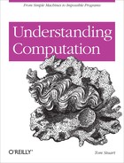
The Game of Life proceeds in a series of steps like a finite state machine. At every step, each cell may potentially change from alive to dead, or vice versa, according to rules that are triggered by the current state of the cell itself and the states of its neighbors. The rules are simple: a living cell dies if it has fewer than two living neighbors (underpopulation) or more than three (overpopulation), and a dead cell comes to life if it has exactly three living neighbors (reproduction).
Here are six examples[63] of how the Game of Life rules affect a cell’s state over the course of a single step, with living cells shown in black and dead ones in white:
Note
A system like this, consisting of an array of cells and a set of rules for updating a cell’s state at each step, is called a cellular automaton.
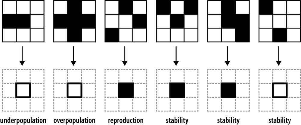
Like the other systems we’ve seen in this chapter, the Game of Life exhibits surprising complexity despite the simplicity of its rules. Interesting behavior can arise from specific patterns of living cells, the best-known of which is the glider, an arrangement of five living cells that moves itself one square diagonally across the grid every four steps:
Many other significant patterns have been discovered, including shapes that move around the grid in different ways (spaceships), generate a stream of other shapes (guns), or even produce complete copies of themselves (replicators).
In 1982, Conway showed how to use a stream of gliders to represent streams of binary data, as well as how to design logical And, Or, and Not gates to perform digital computation by colliding gliders in creative ways. These constructions showed that it was theoretically possible to simulate a digital computer in the Game of Life, but Conway stopped short of designing a working machine:
For here on it’s just an engineering problem to construct an arbitrarily large finite (and very slow!) computer. Our engineer has been given the tools—let him finish the job! […] The kind of computer we have simulated is technically known as a universal machine because it can be programmed to perform any desired calculation.
—John Conway, Winning Ways for Your Mathematical Plays
In 2002, Paul Chapman implemented a particular kind of universal computer in Life, and in 2010 Paul Rendell constructed a universal Turing machine.
Rule 110
Rule 110 is another cellular automaton, introduced by Stephen Wolfram in 1983. Each cell can be either alive or dead, just like the cells in Conway’s Game of Life, but rule 110 operates on cells arranged in a one-dimensional row instead of a two-dimensional grid. That means each cell only has two neighbors—the cells immediately to its left and right in the row—rather than the eight neighbors that surround each Game of Life cell.
At each step of the rule 110 automaton, the next state of a cell is determined by its own state and the states of its two neighbors. Unlike the Game of Life, whose rules are general and apply to many different arrangements of living and dead cells, the rule 110 automaton has a separate rule for each possibility:
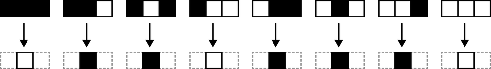
Note
If we read off the values of the “after” cells from these eight rules, treating a dead cell as the digit 0 and a living cell as 1, we get the binary number 01101110. Converting from binary produces the decimal number 110, which is what gives this cellular automaton its name.
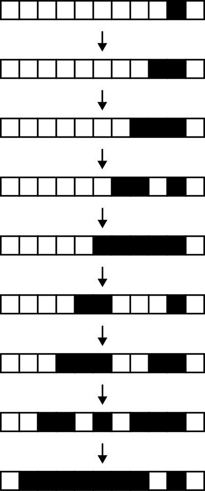
Rule 110 is much simpler than the Game of Life, but again, it’s capable of complex behavior. Here are the first few steps of a rule 110 automaton starting from a single live cell:
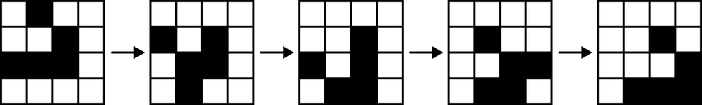
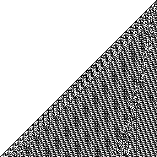
This behavior is already not obviously simple—it’s not just generating a solid line of living cells, for instance—and if we run the same automaton for 500 steps we can see interesting patterns begin to emerge:
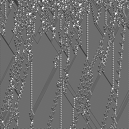
Alternatively, running rule 110 from an initial state consisting of a random pattern of living and dead cells reveals all kinds of shapes moving around and interacting with each other:
The complexity that emerges from these eight simple rules turns out to be remarkably powerful: in 2004, Matthew Cook published a proof that rule 110 is in fact universal. The proof has a lot of detail (see sections 3 and 4 of http://www.complex-systems.com/pdf/15-1-1.pdf) but, roughly, it introduces several different rule 110 patterns that act as gliders, then shows how to simulate any cyclic tag system by arranging those gliders in a particular way.
This means that rule 110 can run a simulation of a cyclic tag system that is running a simulation of a conventional tag system that is running a simulation of a universal Turing machine—not an efficient way to achieve universal computation, but still an impressive technical result for such a simple cellular automaton.
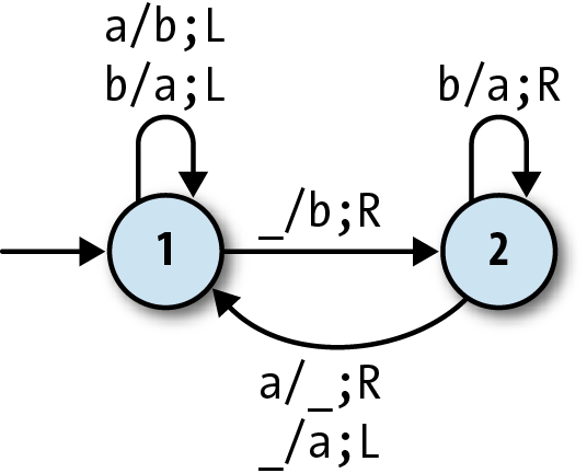
Wolfram’s 2,3 Turing Machine
To complete our whirlwind tour of simple universal systems, here’s one that’s even simpler
than rule 110: Wolfram’s 2,3 Turing machine. It
gets its name from its two states and three characters (a, b, and
blank), which means it has only six rules:
Note
This Turing machine is unusual in that it doesn’t have an accept state, so it never halts, but this is mostly a technical detail. We can still get results out of nonhalting machines by watching for certain behavior—for example, the appearance of a particular pattern of characters on the tape—and treating that as an indication that the current tape contains useful output.
Wolfram’s 2,3 Turing machine doesn’t seem anywhere near powerful enough to support universal computation, but in 2007, Wolfram Research announced a $25,000 prize to anyone who could prove it was universal, and later that year, Alex Smith claimed the prize by producing a successful proof. As with rule 110, the proof hinges on showing that this machine can simulate any cyclic tag system; again, the proof is very detailed, but can be seen in full at http://www.wolframscience.com/prizes/tm23/.
[53] “Hardware” means the read/write head, the tape, and the rulebook. They’re not literally hardware since a Turing machine is usually a thought experiment rather than a physical object, but they’re “hard” in the sense that they’re a fixed part of the system, as opposed to the ever-changing “soft” information that exists as characters written on the tape.
[54] The implementation of TAPE_MOVE_HEAD_LEFT is similar, although it
requires some extra list-manipulation functions that didn’t get
defined in Lists.
[55] The term Turing complete is often used to describe a system or programming language that can simulate any Turing machine.
[56] Because subtraction is the inverse of addition, (x + (y − 1)) + 1 = (x + (y + −1)) + 1. Because addition is associative, (x + (y + −1)) + 1 = (x + y) + (−1 + 1). And because −1 + 1 = 0, which is the identity element for addition, (x + y) + (−1 + 1) = x + y.
[57] Of course the underlying implementation of #recurse itself uses a recursive method definition, but that’s allowed,
because we’re treating #recurse as one of the four
built-in primitives of the system, not a user-defined method.
[58] This second condition prevents us from ever getting into a situation where we need to delete more characters than the string contains.
[59] Doubling a number shifts all the digits in its binary representation one place to the left, and halving it shifts them all one place to the right.
[60] A cyclic tag system rule doesn’t need to say “when the string begins with 1, append the characters 011,” because the first part is assumed—just “append the characters
011” is enough.
[61] Unlike a normal tag system, a cyclic tag system keeps going when no rule applies,
otherwise it would never get anywhere. The only way for a cyclic tag system to stop
running is for its current string to become empty; this always happens when the initial
string consists entirely of 0 characters, for
example.
[62] The resulting sequence of 0s
and 1s is not
meant to represent a binary number. It’s just a string of 0 characters with a 1 character marking a particular
position.
[63] Out of a possible 512: nine cells are involved, and each cell can be in one of two states, so there are 2 × 2 × 2 × 2 × 2 × 2 × 2 × 2 × 2 = 512 different possibilities.