Chapter 5. The Ultimate Machine
In Chapter 3 and Chapter 4, we investigated the capabilities of simple models of computation. We’ve seen how to recognize strings of increasing complexity, how to match regular expressions, and how to parse programming languages, all using basic machines with very little complexity.
But we’ve also seen that these machines—finite automata and pushdown automata—come with serious limitations that undermine their usefulness as realistic models of computation. How much more powerful do our toy systems need to get before they’re able to escape these limitations and do everything that a normal computer can do? How much more complexity is required to model the behavior of RAM, or a hard drive, or a proper output mechanism? What does it take to design a machine that can actually run programs instead of always executing a single hardcoded task?
In the 1930s, Alan Turing was working on essentially this problem. At that time, the word “computer” meant a person, usually a woman, whose job was to perform long calculations by repeating a series of laborious mathematical operations by hand. Turing was looking for a way to understand and characterize the operation of a human computer so that the same tasks could be performed entirely by machines. In this chapter, we’ll look at Turing’s revolutionary ideas about how to design the simplest possible “automatic machine” that captures the full power and complexity of manual computation.
Deterministic Turing Machines
In Chapter 4, we were able to increase the computational power of a finite automaton by giving it a stack to use as external memory. Compared to the finite internal memory provided by a machine’s states, the real advantage of a stack is that it can grow dynamically to accommodate any amount of information, allowing a pushdown automaton to handle problems where an arbitrary amount of data needs to be stored.
However, this particular form of external memory imposes inconvenient limitations on how data can be used after it’s been stored. By replacing the stack with a more flexible storage mechanism, we can remove those limitations and achieve another increase in power.
Storage
Computing is normally done by writing certain symbols on paper. We may suppose this paper is divided into squares like a child’s arithmetic book. In elementary arithmetic the two-dimensional character of the paper is sometimes used. But such a use is always avoidable, and I think that it will be agreed that the two-dimensional character of paper is no essential of computation. I assume then that the computation is carried out on one-dimensional paper, i.e. on a tape divided into squares.
Turing’s solution was to equip a machine with a blank tape of unlimited length—effectively a one-dimensional array that can grow at both ends as needed—and allow it to read and write characters anywhere on the tape. A single tape serves as both storage and input: it can be prefilled with a string of characters to be treated as input, and the machine can read those characters during execution and overwrite them if necessary.
A finite state machine with access to an infinitely long tape is called a Turing machine (TM). That name usually refers to a machine with deterministic rules, but we can also call it a deterministic Turing machine (DTM) to be completely unambiguous.
We already know that a pushdown automaton can only access a single fixed location in its external storage—the top of the stack—but that seems too restrictive for a Turing machine. The whole point of providing a tape is to allow arbitrary amounts of data to be stored anywhere on it and read off again in any order, so how do we design a machine that can interact with the entire length of its tape?
One option is make the tape addressable by random access, labeling each square with a unique numerical address like computer RAM, so that the machine can immediately read or write any location. But that’s more complicated than strictly necessary, and requires working out details like how to assign addresses to all the squares of an infinite tape and how the machine should specify the address of the square it wants to access.
Instead, a conventional Turing machine uses a simpler arrangement: a tape head that points at a specific position on the tape and can only read or write the character at that position. The tape head can move left or right by a single square after each step of computation, which means that a Turing machine has to move its head laboriously back and forth over the tape in order to reach distant locations. The use of a slow-moving head doesn’t affect the machine’s ability to access any of the data on the tape, only the amount of time it takes to do it, so it’s a worthwhile trade-off for the sake of keeping things simple.
Having access to a tape allows us to solve new kinds of problems beyond simply accepting or rejecting strings. For example, we can design a DTM for incrementing a binary number in-place on the tape. To do this, we need to know how to increment a single digit of a binary number, but fortunately, that’s easy: if the digit is a zero, replace it with a one; if the digit is a one, replace it with a zero, then increment the digit immediately to its left (“carry the one”) using the same technique. The Turing machine just has to use this procedure to increment the binary number’s rightmost digit and then return the tape head to its starting position:
Give the machine three states, 1, 2 and 3, with state 3 being the accept state.
Start the machine in state 1 with the tape head positioned over the rightmost digit of a binary number.
When in state 1 and a zero (or blank) is read, overwrite it with a one, move the head right, and go into state 2.
When in state 1 and a one is read, overwrite it with a zero and move the head left.
When in state 2 and a zero or one is read, move the head right.
When in state 2 and a blank is read, move the head left and go into state 3.
This machine is in state 1 when it’s trying to increment a digit, state 2 when it’s
moving back to its starting position, and state 3 when it has finished. Below is a trace of
its execution when the initial tape contains the string '1011'; the character currently underneath the tape head is shown surrounded by
brackets, and the underscores represent the blank squares on either side of the input
string.
| State | Accepting? | Tape contents | Action |
| 1 | no | _101(1)__ | write 0, move
left |
| 1 | no | __10(1)0_ | write 0, move
left |
| 1 | no | ___1(0)00 | write 1, move right,
go to state 2 |
| 2 | no | __11(0)0_ | move right |
| 2 | no | _110(0)__ | move right |
| 2 | no | 1100(_)__ | move left, go to state 3 |
| 3 | yes | _110(0)__ | — |
Note
Moving the tape head back to its initial position isn’t strictly necessary—if we made state 2 an accept state, the machine would halt immediately once it had successfully replaced a zero with a one, and the tape would still contain the correct result—but it’s a desirable feature, because it leaves the head in a position where the machine can be run again by simply changing its state back to 1. By running the machine several times, we can repeatedly increment the number stored on the tape. This functionality could be reused as part of a larger machine for, say, adding or multiplying two binary numbers.
Rules
Let us imagine the operations performed by the computer to be split up into “simple operations” that are so elementary that it is not easy to imagine them further divided. […] The operation actually performed is determined […] by the state of mind of the computer and the observed symbols. In particular, they determine the state of mind of the computer after the operation is carried out.
We may now construct a machine to do the work of this computer.
—Alan Turing, On Computable Numbers, with an Application to the Entscheidungsproblem
There are several “simple operations” we might want a Turing machine to perform in each step of computation: read the character at the tape head’s current position, write a new character at that position, move the head left or right, or change state. Instead of having different kinds of rule for all these actions, we can keep things simple by designing a single format of rule that is flexible enough for every situation, just as we did for pushdown automata.
This unified rule format has five parts:
The current state of the machine
The character that must appear at the tape head’s current position
The next state of the machine
The character to write at the tape head’s current position
The direction (left or right) in which to move the head after writing to the tape
Here we’re making the assumption that a Turing machine will change state and write a character to the tape every time it follows a rule. As usual for a state machine, we can always make the “next state” the same as the current one if we want a rule that doesn’t actually change state; similarly, if we want a rule that doesn’t change the tape contents, we can just use one that writes the same character that it reads.
Note
We’re also assuming that the tape head always moves at every step. This makes it impossible to write a single rule that updates the state or the tape contents without moving the head, but we can get the same effect by writing one rule that makes the desired change and another rule that moves the head back to its original position afterward.
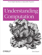
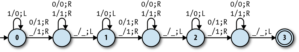
The Turing machine for incrementing a binary number has six rules when they’re written in this style:
When in state 1 and a zero is read, write a one, move right, and go into state 2.
When in state 1 and a one is read, write a zero, move left, and stay in state 1.
When in state 1 and a blank is read, write a one, move right, and go into state 2.
When in state 2 and a zero is read, write a zero, move right, and stay in state 2.
When in state 2 and a one is read, write a one, move right, and stay in state 2.
When in state 2 and a blank is read, write a blank, move left, and go into state 3.
We can show this machine’s states and rules on a diagram similar to the ones we’ve already been using for finite and pushdown automata:
In fact, this is just like a DFA diagram except for the labels on
the arrows. A label of the form a/b;L
indicates a rule that reads character a from the tape, writes character b, and then moves the tape head one square to
the left; a rule labelled a/b;R does
almost the same, but moves the head to the right instead of the
left.
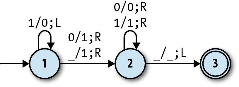
Let’s see how to use a Turing machine to solve a string-recognition problem that
pushdown automata can’t handle: identifying inputs that consist of one or more a characters followed by the same number of bs and cs (e.g., 'aaabbbccc'). The Turing machine that solves this problem has 6
states and 16 rules:
It works roughly like this:
Scan across the input string by repeatedly moving the tape head to the right until an
ais found, then cross it out by replacing it with anX(state 1).Scan right looking for a
b, then cross it out (state 2).Scan right looking for a
c, then cross it out (state 3).Scan right looking for the end of the input string (state 4), then scan left looking for the beginning (state 5).
Repeat these steps until all characters have been crossed out.
If the input string consists of one or more a
characters followed by the same number of bs and cs, the machine will make repeated passes across the whole
string, crossing out one of each character on every pass, and then enter an accept state
when the entire string has been crossed out. Here’s a trace of its execution when the input
is 'aabbcc':
| State | Accepting? | Tape contents | Action |
| 1 | no | ______(a)abbcc_ | write X, move right,
go to state 2 |
| 2 | no | _____X(a)bbcc__ | move right |
| 2 | no | ____Xa(b)bcc___ | write X, move right,
go to state 3 |
| 3 | no | ___XaX(b)cc____ | move right |
| 3 | no | __XaXb(c)c_____ | write X, move right,
go to state 4 |
| 4 | no | _XaXbX(c)______ | move right |
| 4 | no | XaXbXc(_)______ | move left, go to state 5 |
| 5 | no | _XaXbX(c)______ | move left |
| 5 | no | __XaXb(X)c_____ | move left |
| 5 | no | ___XaX(b)Xc____ | move left |
| 5 | no | ____Xa(X)bXc___ | move left |
| 5 | no | _____X(a)XbXc__ | move left |
| 5 | no | ______(X)aXbXc_ | move left |
| 5 | no | ______(_)XaXbXc | move right, go to state 1 |
| 1 | no | ______(X)aXbXc_ | move right |
| 1 | no | _____X(a)XbXc__ | write X, move right,
go to state 2 |
| 2 | no | ____XX(X)bXc___ | move right |
| 2 | no | ___XXX(b)Xc____ | write X, move right,
go to state 3 |
| 3 | no | __XXXX(X)c_____ | move right |
| 3 | no | _XXXXX(c)______ | write X, move right,
go to state 4 |
| 4 | no | XXXXXX(_)______ | move left, go to state 5 |
| 5 | no | _XXXXX(X)______ | move left |
| 5 | no | __XXXX(X)X_____ | move left |
| 5 | no | ___XXX(X)XX____ | move left |
| 5 | no | ____XX(X)XXX___ | move left |
| 5 | no | _____X(X)XXXX__ | move left |
| 5 | no | ______(X)XXXXX_ | move left |
| 5 | no | ______(_)XXXXXX | move right, go to state 1 |
| 1 | no | ______(X)XXXXX_ | move right |
| 1 | no | _____X(X)XXXX__ | move right |
| 1 | no | ____XX(X)XXX___ | move right |
| 1 | no | ___XXX(X)XX____ | move right |
| 1 | no | __XXXX(X)X_____ | move right |
| 1 | no | _XXXXX(X)______ | move right |
| 1 | no | XXXXXX(_)______ | move left, go to state 6 |
| 6 | yes | _XXXXX(X)______ | — |
This machine works because of the exact choice of rules during the scanning stages. For
example, while the machine is in state 3—scanning right and looking for a c—it only has rules for moving the head past bs and Xs. If it hits some
other character (e.g., an unexpected a), then it has no
rule to follow, in which case it’ll go into an implicit stuck state and stop executing,
thereby rejecting that input.
Warning
We’re keeping things simple by assuming that the input can only ever contain the
characters a, b, and
c, but this machine won’t work properly if that’s not
true; for example, it will accept the string 'XaXXbXXXc' even though it should be rejected. To correctly handle that sort
of input, we’d need to add more states and rules that scan over the whole string to check
that it doesn’t contain any unexpected characters before the machine starts crossing
anything off.
Determinism
For a particular Turing machine design to be deterministic, it has to obey the same constraints as a deterministic pushdown automaton (see Determinism), although this time we don’t have to worry about free moves, because Turing machines don’t have them.
A Turing machine’s next action is chosen according to its current state and the character currently underneath its tape head, so a deterministic machine can only have one rule for each combination of state and character—the “no contradictions” rule—in order to prevent any ambiguity over what its next action will be. For simplicity, we’ll relax the “no omissions” rule, just as we did for DPDAs, and assume there’s an implicit stuck state that the machine can go into when no rule applies, instead of insisting that it must have a rule for every possible situation.
Simulation
Now that we have a good idea of how a deterministic Turing machine should work, let’s build a Ruby simulation of one so we can see it in action.
The first step is to implement a Turing machine tape. This implementation obviously has to store the characters that are written on the tape, but it also needs to remember the current position of the tape head so that the simulated machine can read the current character, write a new character at the current position, and move the head left and right to reach other positions.
An elegant way of doing this is to split up the tape into three separate parts—all the characters to the left of the tape head, the single character directly underneath it, and all the characters to its right—and store each part separately. This makes it very easy to read and write the current character, and moving the tape head can be achieved by shuffling characters between all three parts; moving one square to the right, for instance, means that the current character becomes the last character to the left of the head, and the first character to the right of the head becomes the current one.
Our implementation must also maintain the illusion that the tape is infinitely long and filled with blank squares, but fortunately, we don’t need an infinitely large data structure to do this. The only tape location that can be read at any given moment is the one that’s beneath the head, so we just need to arrange for a new blank character to appear there whenever the head is moved beyond the finite number of nonblank characters already written on the tape. To make this work, we need to know in advance which character represents a blank square, and then we can make that character automatically appear underneath the tape head whenever it moves into an unexplored part of the tape.
So, the basic representation of a tape looks like this:
classTape<Struct.new(:left,:middle,:right,:blank)definspect"#<Tape#{left.join}(#{middle})#{right.join}>"endend
This lets us create a tape and read the character beneath the tape head:
>>tape=Tape.new(['1','0','1'],'1',[],'_')=> #<Tape 101(1)>>>tape.middle=> "1"
We can add operations to write to the current tape position[37] and move the head left and right:
classTapedefwrite(character)Tape.new(left,character,right,blank)enddefmove_head_leftTape.new(left[0..-2],left.last||blank,[middle]+right,blank)enddefmove_head_rightTape.new(left+[middle],right.first||blank,right.drop(1),blank)endend
Now we can write onto the tape and move the head around:
>>tape=> #<Tape 101(1)>>>tape.move_head_left=> #<Tape 10(1)1>>>tape.write('0')=> #<Tape 101(0)>>>tape.move_head_right=> #<Tape 1011(_)>>>tape.move_head_right.write('0')=> #<Tape 1011(0)>
In Chapter 4, we used the word configuration to refer to the combination of a pushdown automaton’s state and stack, and the same idea is useful here. We can say that a Turing machine configuration is the combination of a state and a tape, and implement Turing machine rules that deal directly with those configurations:
classTMConfiguration<Struct.new(:state,:tape)endclassTMRule<Struct.new(:state,:character,:next_state,:write_character,:direction)defapplies_to?(configuration)state==configuration.state&&character==configuration.tape.middleendend
A rule only applies when the machine’s current state and the character currently underneath the tape head match its expectations:
>>rule=TMRule.new(1,'0',2,'1',:right)=> #<struct TMRulestate=1,character="0",next_state=2,write_character="1",direction=:right>>>rule.applies_to?(TMConfiguration.new(1,Tape.new([],'0',[],'_')))=> true>>rule.applies_to?(TMConfiguration.new(1,Tape.new([],'1',[],'_')))=> false>>rule.applies_to?(TMConfiguration.new(2,Tape.new([],'0',[],'_')))=> false
Once we know that a rule applies to a particular configuration, we need the ability to update that configuration by writing a new character, moving the tape head, and changing the machine’s state in accordance with the rule:
classTMRuledeffollow(configuration)TMConfiguration.new(next_state,next_tape(configuration))enddefnext_tape(configuration)written_tape=configuration.tape.write(write_character)casedirectionwhen:leftwritten_tape.move_head_leftwhen:rightwritten_tape.move_head_rightendendend
That code seems to work fine:
>>rule.follow(TMConfiguration.new(1,Tape.new([],'0',[],'_')))=> #<struct TMConfiguration state=2, tape=#<Tape 1(_)>>
The implementation of DTMRulebook is almost the
same as DFARulebook and DPDARulebook, except #next_configuration
doesn’t take a character argument, because there’s no
external input to read characters from (only the tape, which is already part of the
configuration):
classDTMRulebook<Struct.new(:rules)defnext_configuration(configuration)rule_for(configuration).follow(configuration)enddefrule_for(configuration)rules.detect{|rule|rule.applies_to?(configuration)}endend
Now we can make a DTMRulebook
for the “increment a binary number” Turing machine and use it to
manually step through a few configurations:
>>rulebook=DTMRulebook.new([TMRule.new(1,'0',2,'1',:right),TMRule.new(1,'1',1,'0',:left),TMRule.new(1,'_',2,'1',:right),TMRule.new(2,'0',2,'0',:right),TMRule.new(2,'1',2,'1',:right),TMRule.new(2,'_',3,'_',:left)])=> #<struct DTMRulebook rules=[…]>>>configuration=TMConfiguration.new(1,tape)=> #<struct TMConfiguration state=1, tape=#<Tape 101(1)>>>>configuration=rulebook.next_configuration(configuration)=> #<struct TMConfiguration state=1, tape=#<Tape 10(1)0>>>>configuration=rulebook.next_configuration(configuration)=> #<struct TMConfiguration state=1, tape=#<Tape 1(0)00>>>>configuration=rulebook.next_configuration(configuration)=> #<struct TMConfiguration state=2, tape=#<Tape 11(0)0>>
It’s convenient to wrap all this up in a DTM class so we can have #step and #run methods, just like we did with the
small-step semantics implementation in Chapter 2:
classDTM<Struct.new(:current_configuration,:accept_states,:rulebook)defaccepting?accept_states.include?(current_configuration.state)enddefstepself.current_configuration=rulebook.next_configuration(current_configuration)enddefrunstepuntilaccepting?endend
We now have a working simulation of a deterministic Turing machine, so let’s give it some input and try it out:
>>dtm=DTM.new(TMConfiguration.new(1,tape),[3],rulebook)=> #<struct DTM …>>>dtm.current_configuration=> #<struct TMConfiguration state=1, tape=#<Tape 101(1)>>>>dtm.accepting?=> false>>dtm.step;dtm.current_configuration=> #<struct TMConfiguration state=1, tape=#<Tape 10(1)0>>>>dtm.accepting?=> false>>dtm.run=> nil>>dtm.current_configuration=> #<struct TMConfiguration state=3, tape=#<Tape 110(0)_>>>>dtm.accepting?=> true
As with our DPDA simulation, we need to do a bit more work to gracefully handle a Turing machine becoming stuck:
>>tape=Tape.new(['1','2','1'],'1',[],'_')=> #<Tape 121(1)>>>dtm=DTM.new(TMConfiguration.new(1,tape),[3],rulebook)=> #<struct DTM …>>>dtm.runNoMethodError: undefined method `follow' for nil:NilClass
This time we don’t need a special representation of a stuck state. Unlike a PDA, a Turing machine doesn’t have an external input, so we can tell it’s stuck just by looking at its rulebook and current configuration:
classDTMRulebookdefapplies_to?(configuration)!rule_for(configuration).nil?endendclassDTMdefstuck?!accepting?&&!rulebook.applies_to?(current_configuration)enddefrunstepuntilaccepting?||stuck?endend
Now the simulation will notice it’s stuck and stop automatically:
>>dtm=DTM.new(TMConfiguration.new(1,tape),[3],rulebook)=> #<struct DTM …>>>dtm.run=> nil>>dtm.current_configuration=> #<struct TMConfiguration state=1, tape=#<Tape 1(2)00>>>>dtm.accepting?=> false>>dtm.stuck?=> true
Just for fun, here’s the Turing machine we saw earlier, for recognizing strings like
'aaabbbccc':
>>rulebook=DTMRulebook.new([# state 1: scan right looking for aTMRule.new(1,'X',1,'X',:right),# skip XTMRule.new(1,'a',2,'X',:right),# cross out a, go to state 2TMRule.new(1,'_',6,'_',:left),# find blank, go to state 6 (accept)# state 2: scan right looking for bTMRule.new(2,'a',2,'a',:right),# skip aTMRule.new(2,'X',2,'X',:right),# skip XTMRule.new(2,'b',3,'X',:right),# cross out b, go to state 3# state 3: scan right looking for cTMRule.new(3,'b',3,'b',:right),# skip bTMRule.new(3,'X',3,'X',:right),# skip XTMRule.new(3,'c',4,'X',:right),# cross out c, go to state 4# state 4: scan right looking for end of stringTMRule.new(4,'c',4,'c',:right),# skip cTMRule.new(4,'_',5,'_',:left),# find blank, go to state 5# state 5: scan left looking for beginning of stringTMRule.new(5,'a',5,'a',:left),# skip aTMRule.new(5,'b',5,'b',:left),# skip bTMRule.new(5,'c',5,'c',:left),# skip cTMRule.new(5,'X',5,'X',:left),# skip XTMRule.new(5,'_',1,'_',:right)# find blank, go to state 1])=> #<struct DTMRulebook rules=[…]>>>tape=Tape.new([],'a',['a','a','b','b','b','c','c','c'],'_')=> #<Tape (a)aabbbccc>>>dtm=DTM.new(TMConfiguration.new(1,tape),[6],rulebook)=> #<struct DTM …>>>10.times{dtm.step};dtm.current_configuration=> #<struct TMConfiguration state=5, tape=#<Tape XaaXbbXc(c)_>>>>25.times{dtm.step};dtm.current_configuration=> #<struct TMConfiguration state=5, tape=#<Tape _XXa(X)XbXXc_>>>>dtm.run;dtm.current_configuration=> #<struct TMConfiguration state=6, tape=#<Tape _XXXXXXXX(X)_>>
This implementation was pretty easy to build—it’s not hard to simulate a Turing machine as long as we’ve got data structures to represent tapes and rulebooks. Of course, Alan Turing specifically intended them to be simple so they would be easy to build and to reason about, and we’ll see later (in General-Purpose Machines) that this ease of implementation is an important property.
Nondeterministic Turing Machines
In Equivalence, we saw that nondeterminism makes no difference to what a finite automaton is capable of, while Nonequivalence showed us that a nondeterministic pushdown automaton can do more than a deterministic one. That leaves us with an obvious question about Turing machines: does adding nondeterminism[38] make a Turing machine more powerful?
In this case the answer is no: a nondeterministic Turing machine can’t do any more than a deterministic one. Pushdown automata are the exception here, because both DFAs and DTMs have enough power to simulate their nondeterministic counterparts. A single state of a finite automaton can be used to represent a combination of many states, and a single Turing machine tape can be used to store the contents of many tapes, but a single pushdown automaton stack can’t represent many possible stacks at once.
So, just as with finite automata, a deterministic Turing machine can simulate a nondeterministic one. The simulation works by using the tape to store a queue of suitably encoded Turing machine configurations, each one containing a possible current state and tape of the simulated machine. When the simulation starts, there’s only one configuration stored on the tape, representing the starting configuration of the simulated machine. Each step of the simulated computation is performed by reading the configuration at the front of the queue, finding each rule that applies to it, and using that rule to generate a new configuration that is written onto the tape at the back of the queue. Once this has been done for every applicable rule, the frontmost configuration is erased and the process starts again with the next configuration in the queue. The simulated machine step is repeated until the configuration at the front of the queue represents a machine that has reached an accept state.
This technique allows a deterministic Turing machine to explore all possible configurations of a simulated machine in breadth-first order; if there is any way for the nondeterministic machine to reach an accept state, the simulation will find it, even if other execution paths lead to infinite loops. Actually implementing the simulation as a rulebook requires a lot of detail, so we won’t try to do it here, but the fact that it’s possible means that we can’t make a Turing machine any more powerful just by adding nondeterminism.
Maximum Power
Deterministic Turing machines represent a dramatic tipping point from limited computing machines to full-powered ones. In fact, any attempt to upgrade the specification of Turing machines to make them more powerful is doomed to failure, because they’re already capable of simulating any potential enhancement.[39] While adding certain features can make Turing machines smaller or more efficient, there’s no way to give them fundamentally new capabilities.
We’ve already seen why this is true for nondeterminism. Let’s look at four other extensions to conventional Turing machines—internal storage, subroutines, multiple tapes, and multidimensional tape—and see why none of them provides an increase in computational power. While some of the simulation techniques involved are complicated, in the end, they’re all just a matter of programming.
Internal Storage
Designing a rulebook for a Turing machine can be frustrating because of the lack of arbitrary internal storage. For instance, we often want the machine to move the tape head to a particular position, read the character that’s stored there, then move to a different part of the tape and perform some action that depends on which character it read earlier. Superficially, this seems impossible, because there’s nowhere for the machine to “remember” that character—it’s still written on the tape, of course, and we can move the head back over there and read it again whenever we like, but once the head moves away from that square, we can no longer trigger a rule based on its contents.
It would be more convenient if a Turing machine had some temporary internal storage—call it “RAM,” “registers,” “local variables,” or whatever—where it could save the character from the current tape square and refer back to it later, even after the head has moved to a different part of the tape entirely. In fact, if a Turing machine had that capability, we wouldn’t need to limit it to storing characters from the tape: it could store any relevant information, like the intermediate result of some calculation the machine is performing, and free us from the chore of having to move the head around to write scraps of data onto the tape. This extra flexibility feels like it could give a Turing machine the ability to perform new kinds of tasks.
Well, as with nondeterminism, adding extra internal storage to a Turing machine certainly would make certain tasks easier to perform, but it wouldn’t enable the machine to do anything it can’t already do. The desire to store intermediate results inside the machine instead of on the tape is relatively easy to dismiss, because the tape works just fine for storing that kind of information, even if it takes a while for the head to move back and forth to access it. But we have to take the character-remembering point more seriously, because a Turing machine would be very limited if it couldn’t make use of the contents of a tape square after moving the head somewhere else.
Fortunately, a Turing machine already has perfectly good internal storage: its current state. There is no upper limit to the number of states available to a Turing machine, although for any particular set of rules, that number must be finite and decided in advance, because there’s no way to create new states during a computation. If necessary, we can design a machine with a hundred states, or a thousand, or a billion, and use its current state to retain arbitrary amounts of information from one step to the next.
This inevitably means duplicating rules to accommodate multiple states whose meanings
are identical except for the information they are “remembering.” Instead of having a single
state that means “scan right looking for a blank square,” a machine can have one state for
“scan right looking for a blank square (remembering that I read an a earlier),” another for “scan right looking for a blank square (remembering
that I read a b earlier),” and so on for all possible
characters—although the number of characters is finite too, so this duplication always has a
limit.
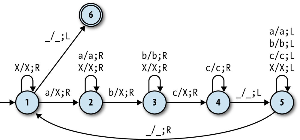
Here’s a simple Turing machine that uses this technique to copy a character from the beginning of a string to the end:
>>rulebook=DTMRulebook.new([# state 1: read the first character from the tapeTMRule.new(1,'a',2,'a',:right),# remember aTMRule.new(1,'b',3,'b',:right),# remember bTMRule.new(1,'c',4,'c',:right),# remember c# state 2: scan right looking for end of string (remembering a)TMRule.new(2,'a',2,'a',:right),# skip aTMRule.new(2,'b',2,'b',:right),# skip bTMRule.new(2,'c',2,'c',:right),# skip cTMRule.new(2,'_',5,'a',:right),# find blank, write a# state 3: scan right looking for end of string (remembering b)TMRule.new(3,'a',3,'a',:right),# skip aTMRule.new(3,'b',3,'b',:right),# skip bTMRule.new(3,'c',3,'c',:right),# skip cTMRule.new(3,'_',5,'b',:right),# find blank, write b# state 4: scan right looking for end of string (remembering c)TMRule.new(4,'a',4,'a',:right),# skip aTMRule.new(4,'b',4,'b',:right),# skip bTMRule.new(4,'c',4,'c',:right),# skip cTMRule.new(4,'_',5,'c',:right)# find blank, write c])=> #<struct DTMRulebook rules=[…]>>>tape=Tape.new([],'b',['c','b','c','a'],'_')=> #<Tape (b)cbca>>>dtm=DTM.new(TMConfiguration.new(1,tape),[5],rulebook)=> #<struct DTM …>>>dtm.run;dtm.current_configuration.tape=> #<Tape bcbcab(_)>
States 2, 3, and 4 of this machine are almost identical, except they each represent a machine that is remembering a different character from the beginning of the string, and in this case, they all do something different when they reach the end.
Note
The machine only works for strings made up of the characters
a, b, and c;
if we wanted it to work for strings containing
any alphabetic characters (or alphanumeric
characters, or whatever larger set we chose), we’d have to add a lot
more states—one for each character that might need to be
remembered—and a lot more rules to go with them.
Exploiting the current state in this way allows us to design Turing machines that can remember any finite combination of facts while the tape head moves back and forth, effectively giving us the same capabilities as a machine with explicit “registers” for internal storage, at the expense of using a large number of states.
Subroutines
A Turing machine’s rulebook is a long, hardcoded list of extremely low-level instructions, and it can be difficult to write these rules without losing sight of the high-level task that the machine is meant to perform. Designing a rulebook would be easier if there was a way of calling a subroutine: if some part of the machine could store all the rules for, say, incrementing a number, then our rulebook could just say “now increment a number” instead of having to manually string together the instructions to make that happen. And again, perhaps that extra flexibility would allow us to design machines with new capabilities.
But this is another feature that is really just about convenience, not overall power. Just like the finite automata that implement individual fragments of a regular expression (see Semantics), several small Turing machines can be connected together to make a larger one, with each small machine effectively acting as a subroutine. The binary-increment machine we saw earlier can have its states and rules built into a larger machine that adds two binary numbers together, and that adder can itself be built into an even larger machine that performs multiplication.
When the smaller machine only needs to be “called” from a single state of the larger one, this is easy to arrange: just include a copy of the smaller machine, merging its start and accept states with the states of the larger machine where the subroutine call should begin and end. This is how we’d expect to use the incrementing machine as part of an adding machine, because the overall design of the rulebook would be to repeat the single task “if the first number isn’t zero, decrement the first number and increment the second number” as many times as possible. There’d only be one place in the machine where incrementing would need to happen, and only one place for execution to continue after the incrementing work had completed.
The only difficulty comes when we want to call a particular subroutine from more than one place in the overall machine. A Turing machine has no way to store a “return address” to let the subroutine know which state to move back into once it has finished, so superficially, we can’t support this more general kind of code reuse. But we can solve this problem with duplication, just like we did in Internal Storage: rather than incorporating a single copy of the smaller machine’s states and rules, we can build in many copies, one for each place where it needs to be used in the larger machine.
For example, the easiest way to turn the “increment a number” machine into an “add three to a number” machine is to connect three copies together to achieve an overall design of “increment the number, then increment the number, then increment the number.” This takes the larger machine through several intermediate states that track its progress toward the final goal, with each use of “increment the number” originating from and returning to a different intermediate state:
>>defincrement_rules(start_state,return_state)incrementing=start_statefinishing=Object.newfinished=return_state[TMRule.new(incrementing,'0',finishing,'1',:right),TMRule.new(incrementing,'1',incrementing,'0',:left),TMRule.new(incrementing,'_',finishing,'1',:right),TMRule.new(finishing,'0',finishing,'0',:right),TMRule.new(finishing,'1',finishing,'1',:right),TMRule.new(finishing,'_',finished,'_',:left)]end=> nil>>added_zero,added_one,added_two,added_three=0,1,2,3=> [0, 1, 2, 3]>>rulebook=DTMRulebook.new(increment_rules(added_zero,added_one)+increment_rules(added_one,added_two)+increment_rules(added_two,added_three))=> #<struct DTMRulebook rules=[…]>>>rulebook.rules.length=> 18>>tape=Tape.new(['1','0','1'],'1',[],'_')=> #<Tape 101(1)>>>dtm=DTM.new(TMConfiguration.new(added_zero,tape),[added_three],rulebook)=> #<struct DTM …>>>dtm.run;dtm.current_configuration.tape=> #<Tape 111(0)_>
The ability to compose states and rules in this way allows us to build Turing machine rulebooks of arbitrary size and complexity, without needing any explicit support for subroutines, as long as we’re prepared to accept the increase in machine size.
Multiple Tapes
The power of a machine can sometimes be increased by expanding its
external storage. For example, a pushdown automaton becomes more
powerful when we give it access to a second stack, because two stacks
can be used to simulate an infinite tape: each stack stores the
characters from one half of the simulated tape, and the PDA can pop and
push characters between the stacks to simulate the motion of the tape
head, just like our Tape
implementation in Simulation. Any
finite state machine with access to an infinite tape is effectively a
Turing machine, so just adding an extra stack makes a pushdown automaton
significantly more powerful.
It’s therefore reasonable to expect that a Turing machine might be
made more powerful by adding one or more extra tapes, each with its own
independent tape head, but again that’s not the case. A single Turing
machine tape has enough space to store the contents of any number of
tapes by interleaving them: three tapes containing abc, def,
and ghi can be stored together as
adgbehcfi. If we leave a blank square
alongside each interleaved character, the machine has space to write
markers indicating where all of the simulated tape heads are located: by
using X characters to mark the
current position of each head, we can represent both the contents and
the head positions of the tapes ab(c), (d)ef, and g(h)i with the single tape a_dXg_b_e_hXcXf_i_.
Programming a Turing machine to use multiple simulated tapes is complicated, but the fiddly details of reading, writing, and moving the heads of the tapes can be wrapped up in dedicated states and rules (“subroutines”) so that the main logic of the machine doesn’t become too convoluted. In any case, however inconvenient the programming turns out to be, a single-tape Turing machine is ultimately capable of performing any task that a multitape machine can, so adding extra tapes to a Turing machine doesn’t give it any new abilities.
Multidimensional Tape
Finally, it’s tempting to try giving a Turing machine a more spacious storage device. Instead of using a linear tape, we could provide an infinite two-dimensional grid of squares and allow the tape head to move up and down as well as left and right. That would be useful for any situation where we want the machine to quickly access a particular part of its external storage without having to move the head past everything else on it, and it would allow us to leave an unlimited amount of blank space around multiple strings so that each of them can easily grow longer, rather than having to manually shuffle information along the whole tape to make space whenever we want to insert a character.
Inevitably, though, a grid can be simulated with one-dimensional tape. The easiest way is to use two one-dimensional tapes: a primary tape for actually storing data, and a secondary tape to use as scratch space. Each row of the simulated grid[40] is stored on the primary tape, top row first, with a special character marking the end of each row.
The primary tape head is positioned over the current character as usual, so to move left and right on the simulated grid, the machine simply moves the head left and right. If the head hits an end-of-row marker, a subroutine is used to shuffle everything along the tape to make the grid one space wider.
To move up or down on the simulated grid, the tape head must move a complete row to the left or right respectively. The machine can do this by first moving the tape head to the beginning or end of the current row, using the secondary tape to record the distance travelled, and then moving the head to the same offset in the previous or next row. If the head moves off the top or bottom of the simulated grid, a subroutine can be used to allocate a new empty row for the head to move into.
This simulation does require a machine with two tapes, but we know how to simulate that too, so we end up with a simulated grid stored on two simulated tapes that are themselves stored on a single native tape. The two layers of simulation introduce a lot of extra rules and states, and require the underlying machine to take many steps to perform a single step of the simulated one, but the added size and slowness don’t prevent it from (eventually) doing what it’s supposed to do.
General-Purpose Machines
All the machines we’ve seen so far have a serious shortcoming: their rules are hardcoded, leaving them unable to adapt to different tasks. A DFA that accepts all the strings that match a particular regular expression can’t learn to accept a different set of strings; an NPDA that recognizes palindromes will only ever recognize palindromes; a Turing machine that increments a binary number will never be useful for anything else.
This isn’t how most real-world computers work. Rather than being specialized for a particular job, modern digital computers are designed to be general purpose and can be programmed to perform many different tasks. Although the instruction set and CPU design of a programmable computer is fixed, it’s able to use software to control its hardware and adapt its behavior to whatever job its user wants it to do.
Can any of our simple machines do that? Instead of having to design a new machine every time we want to do a different job, can we design a single machine that can read a program from its input and then do whatever job the program specifies?
Perhaps unsurprisingly, a Turing machine is powerful enough to read the description of a simple machine from its tape—a deterministic finite automaton, say—and then run a simulation of that machine to find out what it does. In Simulation, we wrote some Ruby code to simulate a DFA from its description, and with a bit of work, the ideas from that code can be turned into the rulebook of a Turing machine that runs the same simulation.
Note
There’s an important difference between a Turing machine that simulates a particular DFA and one that can simulate any DFA.
Designing a Turing machine to reproduce the behavior of a specific DFA is very easy—after all, a Turing machine is just a deterministic finite automaton with a tape attached. Every rule from the DFA’s rulebook can be converted directly into an equivalent Turing machine rule; instead of reading from the DFA’s external input stream, each converted rule reads a character from the tape and moves the head to the next square. But this isn’t especially interesting, since the resulting Turing machine is no more useful than the original DFA.
More interesting is a Turing machine that performs a general DFA simulation. This machine can read a DFA design from the tape—rules, start state, and accept states—and walk through each step of that DFA’s execution, using another part of the tape to keep track of the simulated machine’s current state and remaining input. The general simulation is much harder to implement, but it gives us a single Turing machine that can adapt itself to any job that a DFA can do, just by being fed a description of that DFA as input.
The same applies to our deterministic Ruby simulations of NFAs, DPDAs and NPDAs, each of
which can be turned into a Turing machine capable of simulating any automaton of that type.
But crucially, it also works for our simulation of Turing machines themselves: by
reimplementing Tape, TMRule, DTMRulebook, and DTM as Turing machine rules, we are able to design a machine that
can simulate any other DTM by reading its rules, accept states, and initial configuration from
the tape and stepping through its execution, essentially acting as a Turing machine rulebook
interpreter. A machine that does this is called a universal Turing machine (UTM).
This is exciting, because it makes the maximum computational power of Turing machines available in a single programmable device. We can write software—an encoded description of a Turing machine—onto a tape, feed that tape to the UTM, and have our software executed to produce the behavior we want. Finite automata and pushdown automata can’t simulate their own kind in this way, so Turing machines not only mark the transition from limited to powerful computing machines, but also from single-purpose devices to fully programmable ones.
Let’s look briefly at how a universal Turing machine works. There are a lot of fiddly and uninteresting technical details involved in actually building a UTM, so our exploration will be relatively superficial, but we should at least be able to convince ourselves that such a thing is possible.
Encoding
Before we can design a UTM’s rulebook, we have to decide how to represent an entire Turing machine as a sequence of characters on a tape. A UTM has to read in the rules, accept states, and starting configuration of an arbitrary Turing machine, then repeatedly update the simulated machine’s current configuration as the simulation progresses, so we need a practical way of storing all this information in a way that the UTM can work with.
One challenge is that every Turing machine has a finite number of states and a finite number of different characters it can store on its tape, with both of these numbers being fixed in advance by its rulebook, and a UTM is no exception. If we design a UTM that can handle 10 different tape characters, how can it simulate a machine whose rules use 11 characters? If we’re more generous and design it to handle a hundred different characters, what happens when we want to simulate a machine that uses a thousand? However many characters we decide to use for the UTM’s own tape, it’ll never be enough to directly represent every possible Turing machine.
There’s also the risk of unintentional character collisions between the simulated
machine and the UTM. To store Turing machine rules and configurations on a tape, we need to
be able to mark their boundaries with characters that will have special meaning to the UTM,
so that it can tell where one rule ends and another begins. But if we choose, say, X as the special marker between rules, we’ll run into problems
if any of the simulated rules contain the character X.
Even if we set aside a super-special set of reserved characters that only a universal Turing
machine is allowed to use, they’d still cause problems if we ever tried to simulate the UTM
with itself, so the machine wouldn’t be truly universal. This suggests we need to do some
kind of escaping to prevent ordinary characters from the simulated machine getting
incorrectly interpreted as special characters by the UTM.
We can solve both of these problems by coming up with a scheme that uses a fixed repertoire of characters to encode the tape contents of a simulated machine. If the encoding scheme only uses certain characters, then we can be sure it’s safe for the UTM to use other characters for special purposes, and if the scheme can accommodate any number of simulated states and characters, then we don’t need to worry about the size and complexity of the machine being simulated.
The precise details of the encoding scheme aren’t important as long as it meets these goals. To give an example, one
possible scheme uses a unary[41] representation to encode different values as different-sized strings of a single
repeated character (e.g., 1): if the simulated machine
uses the characters a, b, and c, these could be encoded in unary as
1, 11, and 111. Another character, say 0, can be used as a marker to delimit unary values: the string acbc might be represented as 101110110111. This isn’t a very space-efficient scheme, but it can scale up to
accommodate any number of encoded characters simply by storing longer and longer strings of
1s on the tape.
Once we’ve decided how to encode individual characters, we need a way to represent the
rules of the simulated Turing machine. We can do that by encoding the separate parts of the
rule (state, character, next state, character to write, direction to move) and concatenating
them together on the tape, using special separator characters where necessary. In our
example encoding scheme, we could represent states in unary too—state 1 is 1, state 2 is 11, and so
on—although we’re free to use dedicated characters to represent left and right (say,
L and R), since we
know there will only ever be two directions.
We can concatenate individual rules together to represent an entire rulebook; similarly, we can encode the current configuration of the simulated machine by concatenating the representation of its current state with the representation of its current tape contents.[42] And that gives us what we want: a complete Turing machine written as a sequence of characters on another Turing machine’s tape, ready to be brought to life by a simulation.
Simulation
Fundamentally a universal Turing machine works in the same way as the Ruby simulation we built in Simulation, just much more laboriously.
The description of the simulated machine—its rulebook, accept states, and starting configuration—is stored in encoded form on the UTM’s tape. To perform a single step of the simulation, the UTM moves its head back and forth between the rules, current state, and tape of the simulated machine in search of a rule that applies to the current configuration. When it finds one, it updates the simulated tape according to the character and direction specified by that rule, and puts the simulated machine into its new state.
That process is repeated until the simulated machine enters an accept state, or gets stuck by reaching a configuration to which no rule applies.
[37] Tape, like Stack, is purely functional: writing to
the tape and moving the head are nondestructive operations that
return a new Tape object rather
than updating the existing one.
[38] For a Turing machine, “nondeterminism” means allowing more than one rule per combination of state and character, so that multiple execution paths are possible from a single starting configuration.
[39] Strictly speaking, this is only true for enhancements that we actually know how to implement. A Turing machine would become more powerful if we gave it the magical ability to instantly deduce the answers to questions that no conventional Turing machine can answer (see Chapter 8), but in practice, there’s no way of doing that.
[40] Although the grid itself is infinite, it can only ever have a finite number of characters written onto it, so we only need to store the rectangular area containing all the nonblank characters.
[41] Binary is base two, unary is base one.
[42] We’ve glossed over exactly how a tape should be represented, but that’s not difficult either, and we always have the option of storing it on a simulated second tape by using the technique from Multiple Tapes.