9

Visual Effects

The game does not currently have all of its features. We’ve gone from concept to blockout, then developed the game into a state where it is playable. This doesn’t mean we are finished quite yet! We need to look at how we can bring more emotional immersion to the player. Luckily for us, Unity provides fantastic assets and tools for us to take the current state of our game and visually turn it up another notch. This is done through various vehicles, such as shaders, particles, and other polishing tools that we will cover in Chapter 12, Final Touches.

These topics are very complex. For now, we will go over the main focus of visual effects by looking at shaders and particles at a high level. Then, we will progress to an overview of their advanced forms. Because we are using the Universal Render Pipeline (URP) for this project, we will go over important tools such as Shader Graph, VFX Graph, and Shuriken. Shader Graph visually displays shader detailing and coding. VFX Graph was created to help you understand the various properties of GPU particles. Shuriken, a CPU-focused particle authoring tool, is available in all render pipelines. We will cover that as well.

In this chapter, the following topics will be covered:

• Visual effects overview
• Shader Graph
• Particle Systems:
  • Shuriken
  • VFX Graph

Visual effects overview

Getting started with visual effects may feel daunting at the onset. We currently have a simple scene. The world won’t feel alive and immersive without time spent making deliberate answers to questions needing to be solved to progress the narrative and design of the game.

Throughout this book, you’ve worked through many general game design questions. You’ve been able to answer them yourself and may use them for any project you may want to work on. Then, you were given the answers we discovered ourselves while creating this project and how it would move forward. We had a pretty good idea of what the feel would be for the player: fantasy exploration in the simplest of terms. We now need to be able to go through our scene and find areas in which we need a touch more fantasy. Exploration is done through the mechanics and narrative design.

Fantasy is a broad term. We could have gone with any theme really. We decided to push through this vague starting point and found a theme of light science fiction focused on an ancient race. These beings hold onto the power of the celestial bodies of the natural space surrounding them. Working with nature, they at some point constructed a cave the player will explore. We need to come up with a way to embody this storytelling through visual gameplay, and the player accepting themself as the main character of this world is what we are aiming for.

To carry out this visual storytelling, we need to incorporate the multiple visual effects tools available in Unity. Shader Graph allows us to build shaders that can have interesting properties that play with lights and twinkling effects in various ways. Shuriken provides us with particle systems to add ambient dust, glowing particles around bioluminescent plants, and simple details of other fantasy elements. VFX Graph allows us to push simple particles to the limit and bring GPU systems into play. By pushing GPU systems into play, VFX Graph will give us the ability to use many particles. Though this isn’t practical, you could spawn tens of millions of particles. Finally, we will use the lighting in Unity to provide hints to the player for where to look and set the mood and tone of the current action, system, or place.

To start this chapter, we will be laying the foundation of terms and going over the individual visual effects tools in detail. After these explanations, we can then expand upon how we incorporate the tools that Unity has to offer into our workspace to create a visually immersive environment. Moving forward, this section may become a useful reference point to come back to re-familiarize yourself with the tools and their purpose.

Shader Graph

Shader Graph is a visual scripting tool designed to allow artist-driven shader creation. Shaders are scripts that inform the graphics pipeline how to render materials. A material is an instance of a shader with parameters set for a certain mesh inside of a GameObject. A simple example of this could be leather. If you think of leather, you could probably think about many different types of leather. What color is it? Is it shiny? Does it have a unique texture? All of these options are parameters in the shader that can be set in the material to render the object properly.

In Unity, a shader is written in High-Level Shader Language (HLSL). Knowing how to properly write this code requires a detailed understanding of the graphics pipeline in your computer and can be a bit daunting to get going. The graphics pipeline is a complex conceptual model. Simplified, the computer goes through layers and stages to understand what 3D visual graphics are in a scene, then takes that information and renders those visuals to a 2D screen.

In fact, just reading the paragraph above might’ve seemed a bit confusing. This is natural. There are many moving parts here and we will break this down within this portion of the chapter. In an effort to not dive in too deep with HLSL, we will be focusing purely on Shader Graph. If after spending time in Shader Graph you want to move into a more technical position, we recommend learning HLSL and handwriting shaders. Once you have learned HLSL and handwriting shaders you will have a solid foundation of general shader creation.

Let’s go through the setup of Shader Graph first, then how to create a shader. We should then take some time to talk about basic and commonly used nodes that are used to create shaders. Nodes are a visual representation of a block or chunk of code. These nodes can be linked together to create larger functions of visually layered effects.

Setup

We have been talking about using the URP project, which should automatically have Shader Graph installed on it. If it isn’t installed, you can easily install it by heading to the Package Manager and installing it from the Unity Registry packages.

Figure 9.1 below shows what’s needed to install Shader Graph properly.

If you have a green checkmark like in the figure below, then it is installed already!

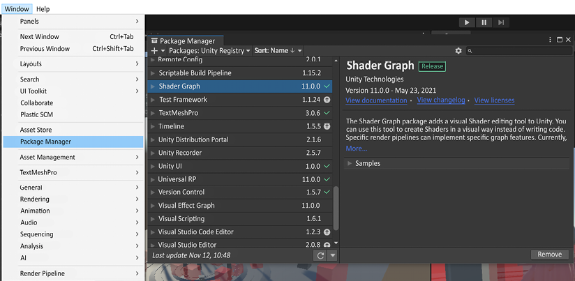
Figure 9.1: Checking if Shader Graph is installed

Now that we have either installed Shader Graph or verified it’s installed, let’s move on to creating your first shader.

Creation

Right-clicking in an open area of your project window gives you the marking menu for that space. We want to make a new shader, so we mouse over Create > Shader > Universal Render Pipeline and then get four options. These four options are the basics from URP that automatically set up the shader settings for you. Refer to Figure 9.2 for the path to follow to create your shader.

Figure 9.2: Path to create a shader in Unity Editor

You may be wondering, “Which one should I choose?” If so, that is a great question. Let’s go over all four of these types just in case you want to mess around with any of the other types after we move along with our choice. From top to bottom we have Lit, Sprite Lit, Sprite Unlit, and Unlit Shader Graphs to work with. Let’s go through each of these types in that order.

Lit Shader Graph

The Lit Shader Graph lets you render 3D objects with real-world lighting information. The shaders that use this will be using a Physically Based Rendering (PBR) lighting model. A PBR model allows 3D surfaces to have a photo-realistic quality of materials like stone, wood, glass, plastic, and metals across various lighting conditions. With the Lit Shader’s assistance, lighting and reflections across these objects can adhere to dynamic shifts, such as bright light to a dark cave environment, accurately.

Sprite Lit Shader Graph

URP comes with a 2D rendering and lighting system. This system would be used in this graph type as the items that this shader would be rendered on would be sprites. A sprite is a two-dimensional bitmap (an array of binary data that represents the color of each pixel) that is integrated into a larger scene. This will allow the sprites to take in the needed lighting information.

Sprite Unlit Shader Graph

This is similar to the Shader Lit Shader Graph above, but the difference with the Sprite Unlit Shader Graph is that it is considered always fully lit and will take in no lighting information. This graph also only uses the 2D rendering and lighting system in the URP.

Unlit Shader Graph

The unlit type of graph for URP uses the 3D PBR lighting model like the Lit Shader Graph type. The major difference is that it won’t take in lighting information. This is the most performant shader in URP.

Shader Graph interface

Choose the Lit Shader Graph type for our Shader Graph. When you right-click in the project window, a new shader file will be created. Double-clicking this file will open the Shader Graph window.

There are some pieces we should go over so you can understand what is covered in the following subsections. We need to go over the Master Stack, Blackboard, Graph Inspector, Main Preview, and then Nodes. In Figure 9.3 below, four out of five of these sections are displayed. We will be going over them in detail in this chapter.

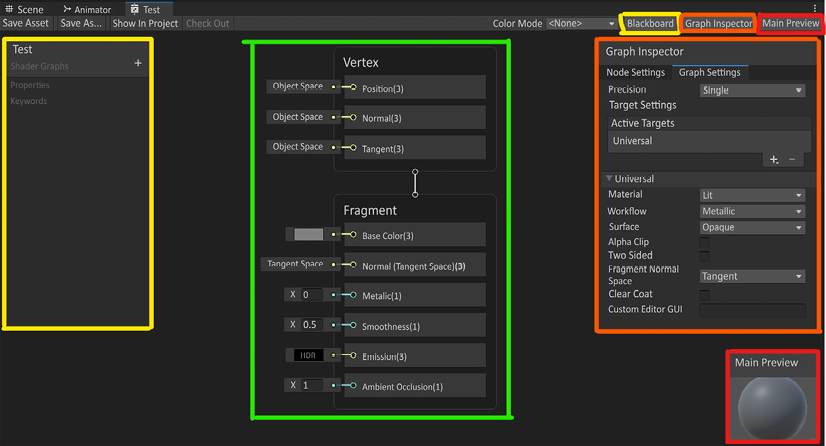
Figure 9.3: Shader Graph window breakdown

Master Stack

The green-outlined item in Figure 9.3 is the Master Stack. There are two sections to the Master Stack, Vertex and Fragment. The Vertex block of the Master Stack contains instructions to the actual vertexes of the 3D object that the material with this assigned shader will be manipulated. Within this block, you can affect the vertex’s Position, Normal, or Tangent attribute. These three attributes occur everywhere in a 2D and 3D environment. Position represents a vertex’s location in object space. Normal is used to calculate which direction light reflects off or is emitted out from the surface. Tangent alters the appearance of vertexes on your surface to define the object’s horizontal (U) texture direction.

In our case, we do not need to change any of the vertex attributes, so we will move on to the fragment shader portion and leave the object space alone.

Fragment instructions can be thought of as possible pixels on your screen. We can affect the pixels depending on the changes made to the inputs to the stack. The attributes that are listed in the fragment shader depend on the shader type we choose when making the shader.

The blocks inside of the Fragment stack are called Fragment Nodes. If you do not need a particular Fragment Node, you can remove it by right-clicking on the Fragment Node individually and selecting Delete. You can also add other Fragment Nodes to the stack by right-clicking the bottom of the Fragment frame and selecting Add Node.

In Figure 9.4, you can see a selection of all the node choices to add to the stack. If your shader isn’t set up to accept those new Fragment Nodes, they will be gray and not usable. For now, let’s go through the Lit Shader Fragment options.

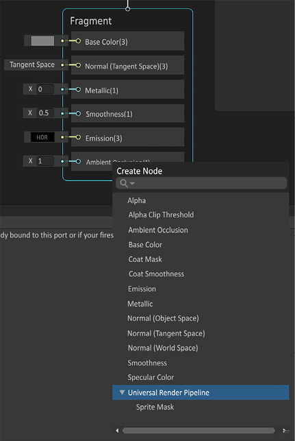
Figure 9.4: Fragment Node options

The Fragment Nodes in the Fragment stack represent the pixels that will potentially be displayed in clip space or on your screen. 3D objects also have a 2D representation of their faces in the form of UVs. UVs are a two-dimensional texture representation of a 3D object. UVs have a flat, 2D axis, 0 (U) to 1 (V) graph. This particular UV graph is a representation of each vertex on this UV plane stretched over a 3D object. The UV graph is also called a UV texture space.

Looking at Figure 9.5 below, you can see that the geometry has been unwrapped to make it flat. This is like papercraft or origami. Knowing how this works sets up the concept of how shaders can manipulate not only the vertex of a mesh but also the color of the faces.

Figure 9.5: Basic mesh, UV layout, gradient on base color

We wanted to show you how we achieved the gradient within Shader Graph for Figure 9.5. Though this isn’t the simplest graph we could’ve started with, it does a good job of breaking down some key concepts early.

If you look at Figure 9.6 below, you will see our graph to build a gradient that we placed in the Base Color. The gradient is then applied to the 0-1 space of the 3D object we assigned this material with this shader. It is not a complex shader as it has hardcoded gradients coming from the UV node.

We will add more complexity to the parameters we make in the Blackboard in the next section.

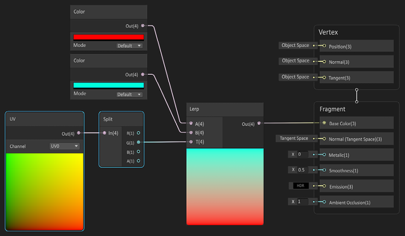
Figure 9.6: Test gradient shader

We will be breaking down commonly used nodes in the next part of this chapter. For now, a quick explanation of what we are doing will help break this down.

Base color

We are taking the UV’s 0-1 space, represented here with two gradients, x and y in the Red and Green channels. Red and Green channels are a part of color space; there are Red (R), Green (G), Blue (B), and Alpha (A) channels. RGB represents the color values. The Alpha channel indicates the opacity of each pixel, from 0 (fully transparent) through to 1 (opaque).

We’ve seen that the 0-1 space starts from the bottom left and ends linearly in the top right in Unity. This means that the Green channel will be a linear gradient from bottom to top. Splitting off that channel allows us to manipulate the 0-1 in a Lerp node, with red replacing black and teal replacing white. There is a lot going on throughout the next few sections, but stick with it! As we break down the nodes, it will be much easier to follow per node.

Normal

Normals tell each fragment how they are supposed to react to light that hits the face.

This is extremely useful to add detail to a face without changing the silhouette, reducing the number of polygons needed for higher detail. Looking at Figure 9.7 below, you can see that it looks as though there are bumps pulled out of the cube. This isn’t a color change; this is light reacting to the surface of the faces. If you look closely, there are no protrusions on the edges. This is because the shape of the cube didn’t change. This is just a cube that acts as it does because of the normal maps.

Figure 9.7: Normals on a cube

On the left side of Figure 9.7, the left cube is blue due to the normal map using its color scheme from the RGB channels in the tangent space. This means that a flat normal map would represent 0, 0, 1. Red and Green channels are used to represent the shifts in how the light should act on either the x tangent or the y tangent. When we work with materials in Chapter 12, Final Touches, we will go further into detail about the functions of a normal map.

Metallic

Metallic is exactly what it sounds like. This is how metallic the material is! That isn’t a great definition though, so let’s try to break it down a little.

The metallic field is a scaler float from 0 to 1, with 0 being not metallic and 1 being bare metal. Metallic materials take in their surrounding environment’s color. In Figure 9.8 we have four spheres with four different settings for their material properties. We’re only using the URP/Lit shader that comes with URP out of the box to test these out. For this section we will only look at the left two spheres. The far-left sphere is white and the metal setting is set to 0. This material is not taking in any of the environment’s color. It’s only taking in lighting information and its base color of white.

The second sphere, though it still has white for a base color, has the metallic setting set to 1. The smoothness is set to 0.5 to be neutral, which you will hear more about shortly. If you look closely the second sphere has the Unity default skybox in the color. Now we need to throw in smoothness to this material.

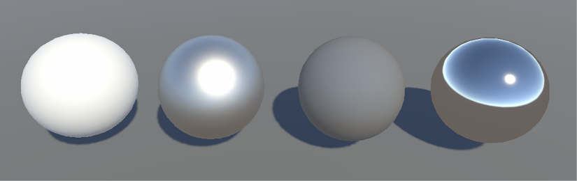
Figure 9.8: From left to right: No metal, all metal, all metal not smooth, all metal all smooth

Smoothness

Continuing with Figure 9.8, we will move on to the right two spheres. The third sphere from the left is very interesting. This one has a base color of white, the metal setting set to 1, and smoothness set to 0. This means that the entire sphere is fully diffused! Diffused in this instance means that all the colors of the environment are blended across the whole sphere, leading to an almost perfect true neutral gray. The fourth sphere is the same, but smoothness is set to 1. This means that the entire sphere is reflecting the direct environment.

Emissive

For an object to emit or radiate light you look toward an emissive map. The purpose of an emissive map is to be able to push colors to have brighter values than 1. Pushing past the value of 1 allows that part of your object to glow brightly. This is useful for lava, sci-fi lights, or anything you want to emit brightness. Otherwise, the Fragment Node defaults to black and no emission is created.

Figure 9.9: Left is no emission, right has emission with 2.4 intensity, no bloom

This doesn’t look like an emissive glowing mushroom! This is due to emission needing a post-processing volume. To do this, create an empty GameObject and name it _PostProcess. We’re naming it this to give it a distinctly different name. Using the underscore as a prefix, we’re letting our developers know that this object houses logic only. There aren’t GameObjects for use in the game itself. Then add a Volume component, seen below in Figure 9.10.

Figure 9.10: Volume added to post-process GameObject

We’re not done yet! We need to add a profile and an override to get our bloom set up. Pressing the New button on the right-hand side of the Volume component will create a profile for your settings to be added to. This allows you to store those settings for other scenes if you need to. When you add a profile, you will then be able to add an override.

We want to click on Add Override, then Post Process, and finally Bloom. Then select the Intensity Boolean checkbox to allow for intensity to be changed. Change it to 1. The settings are shown below in Figure 9.11.

Figure 9.11: Bloom override for post-processing volume

Now we see it emitting light around the mushroom on the screen. This isn’t adding light into the scene; it is only adding a brightness value outside of the mesh to the render on the screen.

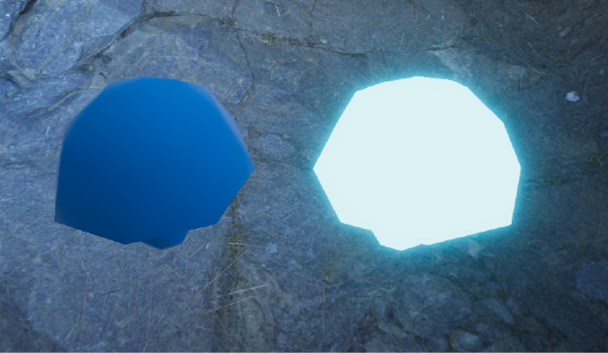
Figure 9.12: Left: no emissive, Right: emissive and bloom set up

We have a shiny, glowing mushroom! Go forth and add emission to things! We will now look into Ambient Occlusion.

Ambient Occlusion

The point of Ambient Occlusion (AO) is to add dark spots to sections to show creases. This adds a nice, clean effect of shadows even if there aren’t any specific lights making shadows. AO is designed for light at all angles. This attribute expects values from 0 to 1. If you do not have an AO map for your model, it’s best to leave it at 1. In Chapter 12, Finishing Touches, we will be working with Myvari’s material, which will have an AO map to go over.

This was the master stack in summary. Each of the attributes on the stack can be used to provide unique shaders. Something that helps with even more customization is the Blackboard part of Shader Graph.

Blackboard

The Blackboard allows the user to create properties and keywords to use in shaders that can be dynamically changed in various ways. Properties can be used within the shader or be exposed to the material in the Inspector using the Exposed checkbox.

You can locate the Blackboard button on the top right of the Shader Graph window. Once you click this button, Blackboard will open its own separate UI.

Figure 9.13: Variable types available in the Blackboard

There are 16 available data types that can be created. These data types can be changed through scripting during runtime as well. Keywords are designed to be changed per material instance during runtime. There are only a few options for this as the compiler needs to account for all the variations. This is handy for things like mobile specifications. You may make an enum (user-defined set of constraints) or list for different systems to change the fidelity (perceptual quality) of the shader to adapt to platform limitations.

Graph Inspector

The Graph Inspector gives you the options for the shader type itself. We chose to start with a URP/Lit shader as our base, which sets specific settings in the Graph Inspector for us. Figure 9.14 below shows the Graph Inspector. These are the settings that are set by default with the URP/Lit.

Figure 9.14: Graph Inspector

Each of these properties available to the shader we are building has great use in certain situations. When we go over using them in, Finishing Touches, we will explain why we are making the changes to the graph settings. For now, understand that the material we chose was the Lit option and it defaults to a metallic opaque workflow. This means that you do not see the color from items behind it as it isn’t transparent.

Main Preview

The Main Preview is an overall glance at what the shader would look like in the game. The default is a sphere.

You can right-click in the window to access multiple options, such as to include a custom mesh, as noted in Figure 9.15 below.

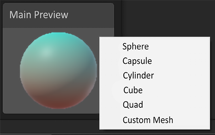
Figure 9.15: Screenshot of the main preview in Shader Graph and its options

Until you plug in some nodes to the Master Stack, this preview will default as a gray sphere. Let’s talk about nodes next!

Nodes

A node is a piece of code that will have at least an output but could also have an input depending on the needs of the node. The purpose is to have a change in data to provide manipulation to the input in the attributes on the master stack. If you can recall back in Figure 9.6, we showed a few nodes: Color, Lerp, Split, and UV. We used them in combination to make the base color be manipulated to show the gradient we made. Figure 9.16 shows a snippet of the screen when we pressed the spacebar down while our mouse was in the empty gray area of the Shader Graph. There are many nodes that can be used together to make many different effects. You can take the time now to search through the node menu and find the nodes we made in Figure 9.6 to play with the gradient yourself.

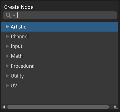
Figure 9.16: Node creation menu

If you took some time to build this out, you may have also opened some of the node groupings and realized that there is a very large number of nodes to choose from. This may cause a little bit of anxiety. Fortunately, we will go over some common nodes that are used in many shaders in the next section.

Commonly used nodes

Below is a simple list of commonly used nodes to make shaders. We want to stress that this isn’t the full list of nodes. In fact, there are over 200 nodes now in Shader Graph 10+. Going over all of them could literally be a book or two. The interesting thing about these sets of nodes is that they can be built up to make some incredible shaders. Something to keep in mind when reading about these is that there may be information in the previous node that helps describe the current node you are reading. Read through them all even if you’re reasonably comfortable with, say, knowing how to add, for example.

Add

To be able to explain Add, we need to make sure you remember that 0 means absence, or the color black in this case. This means that a value of 1 is white. We normalize our values on a 0-1 scale across many applications. You may remember that UV coordinates are also between 0 and 1. This is no mistake! So, if I had two scalars, or Vector1s, and added them, the value would be greater.

Let’s show a quick example: 0.4 + 0.4 = 0.8.

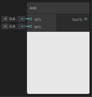
Figure 9.17: Add node

0.4 is a darker-than-medium-gray value. If we add two of them together, we almost get white! 0.8 is 80% to pure white in value, seen in Figure 9.17.

Color

This node is a Vector4 with nice visual sugar on top. Vector4 (0, 0, 0, 0) represents Red, Green, Blue, and Alpha in shader values. Color has an interface for you to select the color you want, and it will set up the RGB values for you with an Alpha slider for that value while outputting a Vector4.

Figure 9.18: Color node

This would be difficult with the Vector4 node as there is no color visual to know what your values need to be.

Lerp

Lerp stands for Linear Interpolation. The Lerp node can be used in many applications. One instance is how we set up a gradient to be used for the base color in Figure 9.6. There are three inputs: A, B, and T. You can think of it as A is 0, B is 1, and T is the driver. The driver (T) is a value of 0-1. However, the value will map to the value of A, B, and the values in between. If T is at 0, it will display an 100% value of what is in A. If T has a value of 1, it will display an 100% value of B. Now, if T is at 0.4, then that will be in between the values of A and B: 40% A and 60% B.

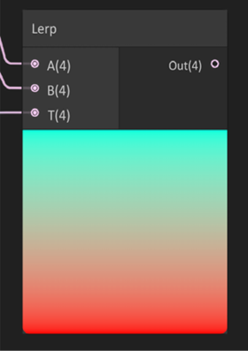
Figure 9.19: Lerp node

This is difficult to visualize with just numbers alone. Luckily, in Figure 9.19 we used the UV to input T as a gradient. This allows us to see the 0-1 going from bottom to top. You are seeing a gradient from A to B from bottom to top.

Multiply

We’ve seen the Add and Lerp nodes; now we need to work through another operation, Multiply. By the nature of basic arithmetic, Multiply will make the value lower.

This is happening because we are in the range of 0-1. Let’s put together an example in Figure 9.20.

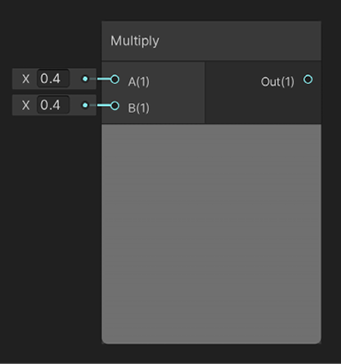
Figure 9.20: Multiply node

We have used the same example we used for the add node but we are using multiplication instead of using addition. Simple math states .4 * .4 = .16.

Sample Texture 2D

This node allows you to take textures you have authored in other Digital Content Creation (DCC) software such as Photoshop and use the color information to manipulate the attributes of the master stack. There are two inputs, the texture you want to sample and the UVs, as seen in Figure 9.21.

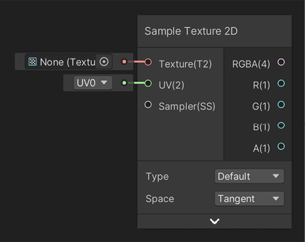
Figure 9.21: Sample Texture 2D

The UV node allows you to manipulate the UV coordinates of your mesh. A nice feature of this node is that it outputs the Vector4 as well as each float individually from the node itself.

Saturate

There may be a time when your values go above 1. This may happen because you are working with multiple nodes that push your values outside the 0-1 range.

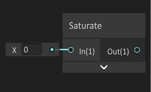
Figure 9.22: Saturate node

If this happens, you can input the data into a saturate node and it will return all of your values within the 0-1 range. Place the float value in the In portion, and the Out value will be normalized to the 0-1 range.

Split

As we saw in the Sample Texture 2D node, the Vector4 was split into individual outputs. This isn’t always the case. The Color node only outputs a Vector4. If you only want to use the Red channel value from Color, how could you get it? You guessed it, a split node. Input a Vector2, 3, or 4 and use whichever channel you desire as a float.

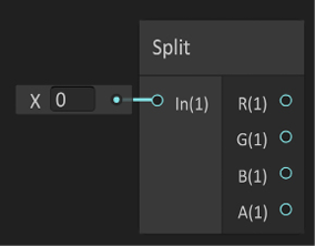
Figure 9.23: Split node

This is very helpful to be able to break out an image that you put four grayscale images onto. We call that channel packing so you can have three images on one texture lookup.

UV

There may be a time when you need to manipulate the UVs of the object you want to render. A reason for this may be that you want to tile the UVs because the scale of the item was larger or smaller than what was intended. Another reason to use the UV node is that it automatically creates horizontal and vertical gradients.

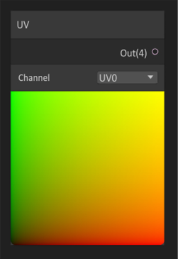
Figure 9.24: UV node

If split, the R channel is the horizontal gradient and the G channel is the vertical gradient.

Vectors

These guys are used everywhere. You’ll notice that a Vector1 is named a Float. Another name for Vector1 is Scalar. Something else you may have noticed is that the outputs are all different colors. Float is cyan, Vector2 is green, Vector3 is yellow, and Vector4 is pink. This is incredibly useful to know the colors as they are shown on the connection lines between the nodes. These nodes are used in infinite use cases. Do you need three points of data? Vector3!

Figure 9.25: Vector nodes

With all of these basic nodes, you can make some powerful shaders to make beautiful materials with. In Chapter 12, Finishing Touches, we will be covering shaders for multiple purposes and showing how we use these nodes to create some nice visual candy. Now let’s move away from Shader Graph and work with Particle Systems so we can add nice visual effects to our experiences.

Particle Systems

When you think of visual effects in a video game, the first thing that pops into your head most likely is the trails of legendary weapons in ARPGs or the amazing explosions from intense first-person-shooter campaigns. Whatever popped into your head, there are systems that allow for these effects to happen. Particle Systems allow for the spawning of meshes with certain rules to create these effects. Two of them in Unity are Shuriken and VFX Graph.

Shuriken

This system is full of features to help spawn 3D meshes (structural collection of vertices, edges, and faces that define a 3D object). You can create fire embers, trails, explosions, smoke, and everything else to help sell the experience that has been defined. As you can see in Figure 9.26 there are a lot of options to go over. We will leave the explanation of this to the examples covered in Chapter 12, Finishing Touches when we create Shuriken-based effects.

Some high-level knowledge of Shuriken to know is that it is a Particle System that uses the CPU to direct the particles.

This limits the amount of particles that can spawn directly on that hardware.

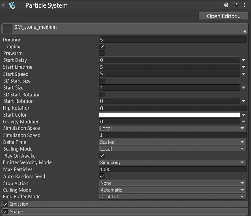
Figure 9.26: Shuriken Particle System

Shuriken is fantastic for particle systems on the CPU, but if you want to have large amounts of particles moving around, VFX Graph is the way to go. This makes GPU-driven particles and can handle many thousands of particles at once.

VFX Graph

Firstly, you will most likely need to install VFX Graph. Open the Package Manager as you have done before and find Visual Effects Graph from within Unity Registry and install it! After you’ve finished this, you will need to create a VFX Graph system. In your project window, right-click and then select Create > Visual Effects > Visual Effects Graph.

Figure 9.27: Installing and creating your first VFX Graph system

Opening VFX Graph will present you with a new window. This window is like the Shader Graph. You’ll notice there is a Blackboard, which we can use to create parameters that can be changed at runtime and is exposed in the inspector.

There is a UI that is unique to the VFX Graph and a few specific terms: Contexts, Blocks, Nodes, and Variables. Contexts are portions of the system broken down, such as Spawning, Initialization, Update, and Output.

Each of these contexts has blocks inside of them and can be added to the contexts by right-clicking. The Spawning context controls how many instances of the system feeds into an Initialize context. Initialize context processes the Spawn Event and engages a new particle simulation. Update context takes in the Initialized particles and executes explicit behaviors upon certain conditions. Output contexts account for the simulation data and render every living particle according to the Output context configuration. However, Output context does not modify simulated data.

The first context is spawning. This context will allow you to add blocks to affect the spawning logic of each system. There are some questions that should be considered here: How many particles should spawn from this system? How quickly should those particles spawn? When are they spawned?

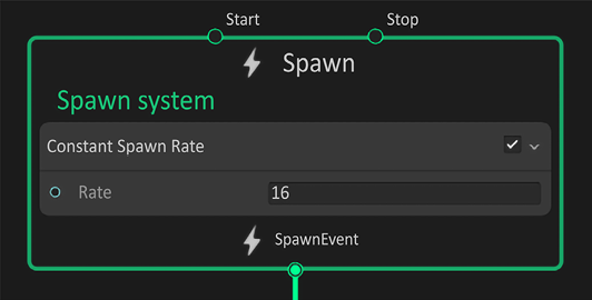
Figure 9.28: Spawn context

After the spawning is completed, you need to have parameters to initialize them with. These blocks answer these types of questions: Where do the particles spawn? Are they spawned moving or do they have velocity? How long does each particle live for?

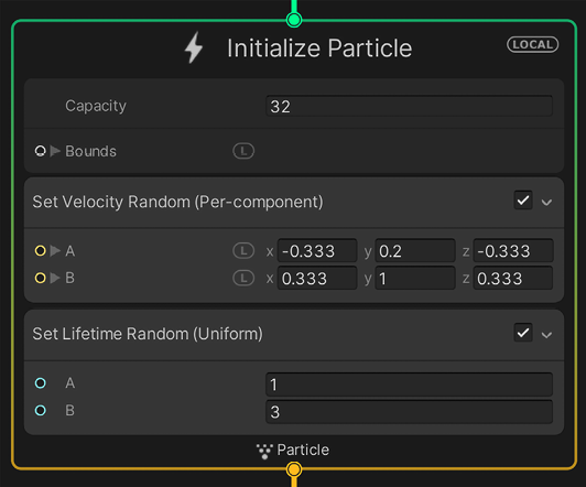
Figure 9.29: Initialize context

Now that you have them spawning, it may be a good idea to add some unique behavior to them as they update, or they will be floating sphere gradients. You can expect this to answer the ultimate question: How will the particles change over time?

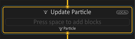
Figure 9.30: Update context

Then finally, as you have an understanding of how many particles there are, where the particles are, and what the particles are doing, you can now decide what they will look like.

The questions are: Which way are the particles facing? What shader is being used?

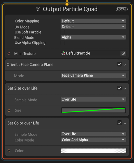
Figure 9.31: Output context

You may have noticed the left side of the blocks sometimes have circle inputs like the Shader Graph. If you thought that you could put some input to this, maybe from nodes, then you’re correct! There are nodes that you can work through to get the right data flowing to the blocks that are in each context.

Nodes

As this was in Shader Graph, the nodes are meant to take data values and manipulate them in a way to get the desired outcome. In VFX Graph’s case the values are meant to be read into one of the blocks as opposed to one of the attributes from the Master Stack. For the most part you will utilize the Operator nodes and variables that are created in the Blackboard to complete the complex maths.

Summary

We learned that visual effects have heavy technical implications through two major sources in Unity: shaders and particles. Taking our time through shaders, we built an example of a material on a 3D object to get the concept down so when we have multiple different scenarios, we can follow how the shader was created. This was done through Shader Graph. After that, we dove into the concept of particles. Shuriken was shown to get a simple understanding of CPU particles and will be used in later chapters to explain the finishing touches. GPU particles are created through VFX Graph; we went over the interface and some vocabulary of VFX Graph so when we use it later, there is an understanding to work off.

Visual effects are a very large topic to master. Mastering these tools takes a long time. Take your time when working through this and fail fast. This will guide you through understanding visual effects.

The next chapter covers the implementation of sound in the game. Sounds are generally overlooked until nearly the end of games, but they are integral to ensuring the product has captivating emotional tie-ins with the environment and the character. We will go over implementations, some sound design, and other sound-focused knowledge points in the next chapter.