CHAPTER 3
Identifying Outliers Using Regression
There will always be a few transactions in every sample whose actual selling price was radically different from the price suggested by the regression trend line (i.e., they are significantly out of alignment with the rest of the market.) The regression analysis not only plots a line that best represents where the market is but also calculates what is referred to as standard error lines. The standard error is a statistical measurement similar to standard deviation. The difference is the standard deviation is a measure of dispersion around a single point in a sample (the mean), whereas the standard error is the same measure dispersion around the regression line. The standard error calculates the upper and lower boundaries between which most of the multipliers (68%) in a sample should fall.
Theoretically, 16% of the sample's transactions should have revenue multipliers that fall above the upper standard error line and 16% of transactions should fall below the lower standard error line. Those transactions that fall outside these boundaries are companies whose selling‐price multiples were so far above or below the rest of the market that the transactional data must be considered flawed or not conforming to the stated standard of value. These “outliers,” as they are referred to, will be removed from our sample of comparables.
The sample from Exhibit 2.3 produced a standard error of 0.10. Exhibit 3.1, below, adds two dotted lines to the graph that are parallel to the trend line reflecting the standard error boundaries. The upper‐boundary line is 0.10 higher (on the Y‐axis) than the trend line, and the lower‐boundary line is 0.10 lower than the trend line.
The remaining 68% of the sample, then, are transactions that best define the market where in all probability our subject will fall. Exhibit 3.1 identified six transactions out of the sample of 24 that fell outside the standard error boundaries (see Exhibit 3.2 below). By removing those outliers, the remaining 18 transactions will generally present a visually compelling argument that the regression trend line is where the market is, not the median.

EXHIBIT 3.1 Standard Error Lines Showing Outliers
EXHIBIT 3.2 Outliers
| SDE% | Actual Multiplier | Predicted Multiplier | Residuals | |
|---|---|---|---|---|
| 1 | 2.9% | 0.136 | 0.213 | –0.077 |
| 2 | 3.5% | 0.179 | 0.225 | –0.045 |
| 3 | 6.9% | 0.264 | 0.296 | –0.032 |
| 4 | 7.0% | 0.232 | 0.297 | –0.064 |
| 5 | 7.4% | 0.244 | 0.304 | –0.060 |
| 6 | 8.3% | 0.433 | 0.323 | 0.110 |
| 7 | 8.6% | 0.479 | 0.330 | 0.149 |
| 8 | 9.4% | 0.310 | 0.346 | –0.036 |
| 9 | 9.4% | 0.469 | 0.346 | 0.123 |
| 10 | 10.6% | 0.320 | 0.370 | −0.051 |
| 11 | 10.9% | 0.415 | 0.377 | 0.037 |
| 12 | 12.2% | 0.400 | 0.405 | −0.005 |
| 13 | 12.4% | 0.678 | 0.409 | 0.269 |
| 14 | 13.2% | 0.480 | 0.426 | 0.054 |
| 15 | 14.2% | 0.312 | 0.445 | −0.134 |
| 16 | 14.5% | 0.406 | 0.452 | −0.046 |
| 17 | 14.6% | 0.235 | 0.454 | −0.219 |
| 18 | 15.4% | 0.452 | 0.471 | −0.019 |
| 19 | 16.4% | 0.538 | 0.491 | 0.048 |
| 20 | 16.6% | 0.451 | 0.496 | −0.045 |
| 21 | 18.3% | 0.595 | 0.530 | 0.065 |
| 22 | 20.0% | 0.619 | 0.565 | 0.054 |
| 23 | 20.1% | 0.536 | 0.566 | −0.031 |
| 24 | 22.0% | 0.560 | 0.606 | −0.046 |
From Exhibit 3.3 we can see that after removing the outliers, the majority of the transactions line up fairly close to the trend line, whereas the median is a constant which is unaffected by the level of a company's profitability.
In Exhibit 3.2 the transactions that are shaded in gray are those that fell outside the standard error lines and are considered outliers. In other words, the absolute value of their residuals was greater than the standard error of 0.10.
In the following chapters you will be shown the printout from Excel's regression that identifies which transactions are outliers.
After the outliers are removed from the sample, a second regression is performed on the smaller refined sample of 18. In Exhibit 3.3 below note that the remaining 18 transactions are clustered tightly about the trend line. Once the outliers are removed, we can see that the majority of the revenue multipliers of the sample of transactions follow a very predictable pattern.
Regression provides us with a statistical measure of the “tightness” or dispersion of that pattern called R2 (R squared). The R2 statistic gives us a statistical measure of the accuracy of the regression that we can use to compare different samples. An R2 ranges from 0 to 1.0. If all the transactions lined up exactly on the regression line, then R2 would be 1.0. If all the transactions' dots are scattered randomly throughout the graph, R2 would be 0.0. A 0.0 would indicate that there is no correlation between a transaction's SDE% profit margin and its corresponding revenue multiplier. Interestingly, as R2 approaches 0.0 the regression line tends to flatten out and at 0.0 the line becomes flat and is approximately the mean of the sample. In other words, if there is no correlation between profitability and the resulting revenue multiplier, the regression will give us a value that is very close to the one calculated by medians used in the conventional methodology.
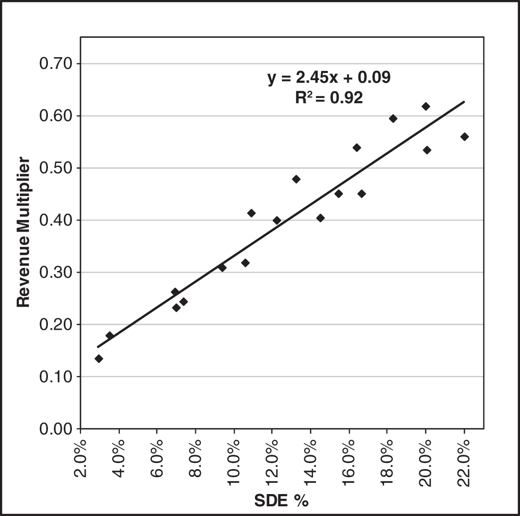
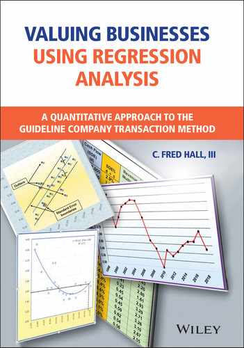
EXHIBIT 3.3 Second Regression with Outliers Removed
In the first regression shown in Exhibit 3.1 note that R2 was 0.53. Generally, any value greater than 0.50 is considered a good correlation between SDE% and the multiplier. However, as we will see in subsequent chapters, even in samples with an R2 as low as 0.25 to 0.30, there still is a visible correlation between SDE% and the corresponding multiplier.
In Exhibit 3.3, the second regression with the outliers removed produced an R2 of 0.92, a significant improvement over the first regression.
The second regression also gives us a new formula for the trend line:
Inserting the 18.3% SDE% from the highly profitable subject company that we used in Exhibit 1.4 we have:
The resulting revenue multiplier of 0.54 produces an estimated value of $648,000. Again, the median revenue multiplier for this highly profitable company suggested a value of only $504,000 while the median cash flow multiplier suggested a $726,000 value (from Exhibit 1.4a following). Even if we averaged those two values (which most appraisers typically do), the average value would be $615,000.
EXHIBIT 1.4a High‐Profit Subject Company
| Example #3 | ||
|---|---|---|
| High‐Profit Subject Company: | ||
| Revenue | $1,200,000 | |
| Cash Flow | $220,000 | 18.3% |
| Using Median Multiplier Values | ||
| $1,200,000 × 0.42 = $504,000 | ||
| $220,000 × 3.30 = $726,000 | ||
Is $648,000 a reasonable value compared to the average median value of $615,000? Our subject's operating profit margin (SDE%) was 18.3%, which is moderately higher than the median of our sample of 12.3%. Given that it is considerably more profitable than most of the 24 transactions in our sample, the higher value of $648,000 is indeed reasonable.