10. Option Investment Profiles
This chapter extends investment profiles to the four basic option variations:
• Long call options
• Short call options (also referred to as written call options)
• Long put options
• Short put options (also referred to as written put options)
Option investment profiles combine standard option profit diagrams with a probability distribution. To provide a comparison benchmark, the graphs also include the stock profit line to highlight the difference between the derivative and its underlying security. This chapter also begins the discussion on leverage and capital allocation, where the intent may not be as clear with options as it is with stocks, and where metrics need to be defined in the context of specific objectives.
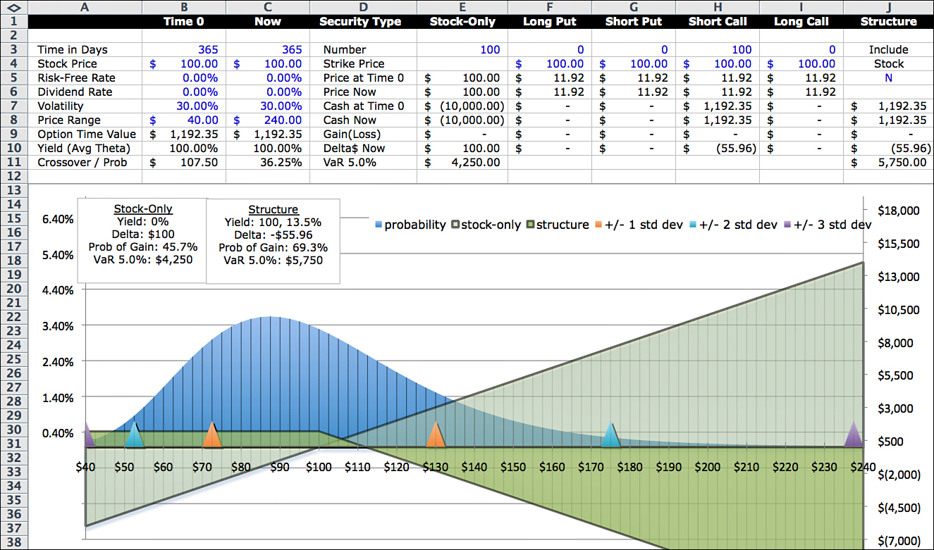
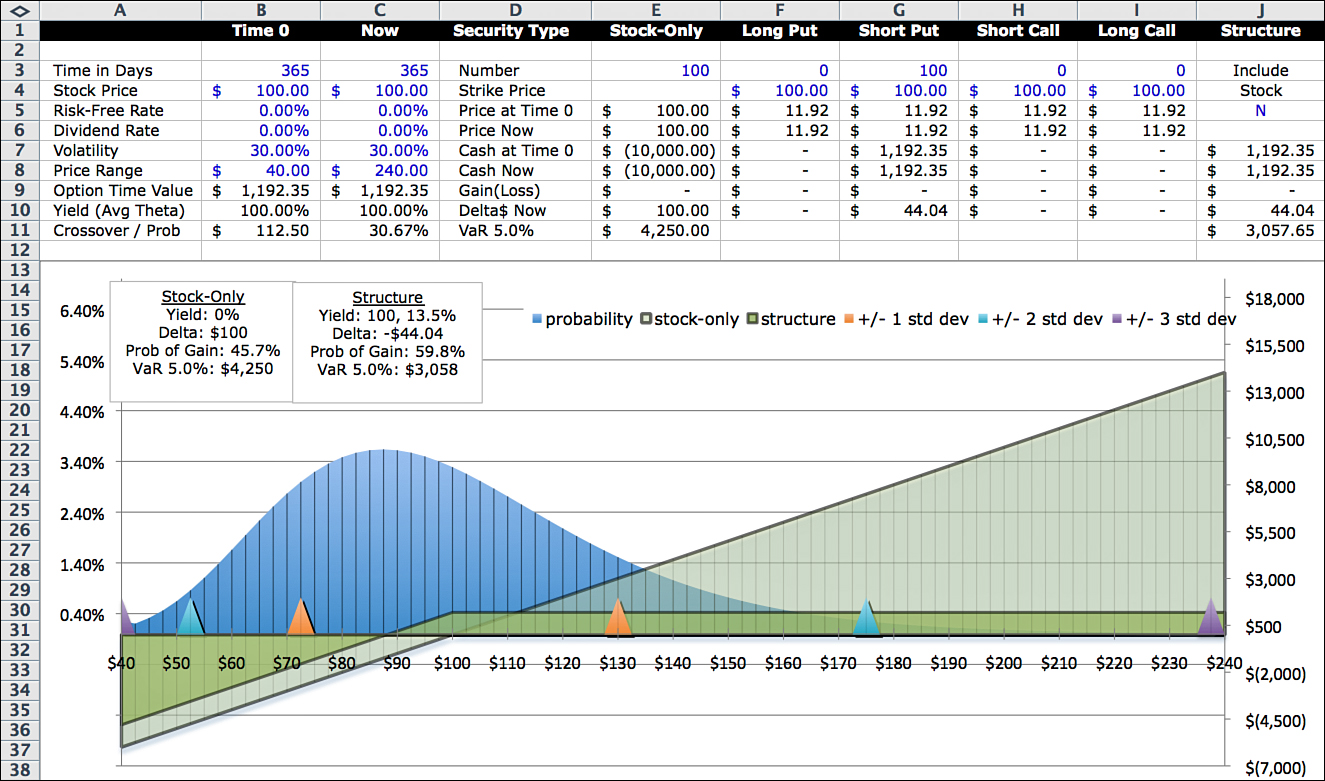
Long Call Option Investment Profile
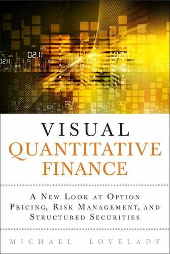
Figure 10.1 compares the stock-only profile to a long call option profile. Assume that the underlying stock and assumptions are the same as in the stock-only example in Figures 8.1 and 8.2: 100 shares of a stock currently trading for $100, a one-year option term, zero interest and dividend rates, a $100 strike price for the option, and implied volatility of 30%.
The profile for the long call option is the darker shaded area. The stock-only profile is the straight-line lighter area. Having both profiles in the graph makes it easier to compare buying an option to what would happen if you bought the stock instead.
You can see one of the advantages of buying a call option on the left side of the graph. If the stock plunges, the most you can lose is $11.92, the amount paid for the option. The breakeven point is $88.08. On the graph, this is the point where the two profit curves intersect. If the stock price is less than $88.08, the option performs better. If the stock price is above $88.08, the stock performs better. With the stock, you make a profit at any price over $100. But with the option, the stock price has to be above $111.92 to make money. On the graph, that point is where the option profit curve crosses the x-axis. The amount paid for the option, $11.92, is represented by the vertical distance between the two profit lines. This distance is the visual representation of the time value of the option.
Option Time Value
When you buy a call option, you can think of the price as being composed of two parts: intrinsic value and time value. Intrinsic value is the difference between the stock price and the strike price. It is the amount by which the option is in-the-money. The time value is the remainder. As an example, let’s say you pay $15 for a call option with a $95 strike price, and the stock price is $100. The intrinsic value is $5, and the time value is $10. Time value is a measure of how much you will make on the option if the stock price stays constant at $100. In other words, time value isolates the effect of the passage of time versus changes in the stock price.
In Figure 10.1, the stock price and the strike price are the same, so the entire value of the option is time value. One of the questions I like to ask with options is:
Am I paying for time, or am I being paid for time—and how much?
The answer, in this case, is: I am paying for time. The amount is $1,192.00. In other words, if I buy the call option contract for $1,192.00 and the stock price at expiration is the same as it is now ($100), I will have paid $1,192.00 for “time.”
Capital at Risk
There is an important distinction between stocks and options. With stocks, both the intent and the capital allocated to a trade are normally understood. If an investor or trader believes a stock is going up, they buy it; or if they think it is going down, they either avoid it or short it. The capital allocated to the position is somewhat defined by how much it costs. Of course, margin accounts allow for some leverage, but it is low compared to the leverage available with options.
With options, the intent and the amount of capital may not be as clear. Therefore, the metrics associated with options are often more meaningful in the context of specific objectives. For instance, for long-term strategic investing, options may act as stock substitutes, insurance, or to generate income or change risk exposures for an existing position. In this context, it is natural to compare the behavior of the option to the behavior of the stock and portfolio capital allocated to the stock position.
On the other hand, in the context of tactical trading, options can be used to create leverage or make short-term directional bets. In that context, it is better to measure option behavior as a stand-alone instrument and define risk and reward metrics differently. In either case, the investment profile gives you the framework to ask and answer a broad range of questions. The idea behind the investment profile is to accommodate both perspectives by presenting options as standalone instruments and in comparison to the underlying stock.
What about the percentage gain or loss in this example? Let’s just look at the case where the stock price at expiration is the same as when the option was purchased, or $100. If you look at the option as speculation, then you would lose 100% of the money used to buy the option. If you look at the option as a stock substitute, and you put aside the $10,000 you would have used to buy the stock and kept it in cash, then you might look at the loss as 11.92% of the amount allocated to this position.
If you use the option for leverage and, instead of buying one contract, you bought eight of them (approximately $10,000 ÷ $11.92) and kept no money in cash, you would definitely think of this as a 100% loss of premium. This is one example of how the metrics need to be interpreted in light of the intent and capital at risk.
In Figure 10.1, the yield calculated in Cells B10 and C10 of –11.92% assume that $10,000 is the capital allocated to the trade, so $10,000 is used in the denominator of the fraction. Some people prefer to use a different definition of capital such as VaR or maximum loss. This is one of those metrics that is not straightforward and depends on the context of the investment or trade. Because the main focus of this book is the comparison of stock positions to a structured security that includes the underlying stock, capital at risk will normally be defined as the net amount invested in the structured security.
Fiduciary Calls and Protective Puts
To make the distinction between stock substitution and speculation, sometimes the term fiduciary call is used. A fiduciary call refers to the combination of cash (or a bond) plus a long call option. A fiduciary call makes it clear that either cash or a bond is being held as capital on the position.
A similar distinction applies to puts. The term protective put refers to the combination of a long stock position and a long put option. A protective put makes it clear that the put is being used as insurance against the associated long stock position rather than as a speculative bet on a decline in the price of the stock, which could be done without holding the stock.
The investment profile of a fiduciary call and a protective put is identical. This is one example of put–call parity, a concept covered in more detail in Chapter 11, “Covered Calls, Condors, and SynAs.”
Annualized Average Theta
Theta is the time decay of an option occurring in one day. It is possible to calculate theta by formula, or you can do it by changing the days until expiration from 365 to 364 in the model. In addition to daily theta, I like to track another number. I call it annualized average theta, and it is displayed in Cells B10 and C10.
Annualized average theta is the time value of the option (in Cells B9 and C9) divided by the number of days left until expiration and then annualized. It is expressed as a percentage of the capital allocated to the position. In this case, with exactly one year left on the option term, it is already annualized; so average theta is –$1,192 ÷ $10,000 = –11.92%. This means we are paying for time at an average rate of 11.92% annually for holding this option. The negative sign indicates that we are paying for time. A positive sign indicates we are being paid.
Delta
The delta of this option position of 100 shares is $55.96. As long as there is any time left before option expiration, the value of an option will not move dollar for dollar with the underlying security. If the underlying stock price increases by $1, the stock position increases in value by $100 for the 100 share position. Delta of $55.96 means that the value of the option position increases by $55.96, or 55.96% ($55.96 ÷ $100.00) of the stock increase. After all, there is still a year for the stock price to increase above the strike price. Understanding the immediate and lagged effects on changes in value is critical to understanding options. Delta changes with the time remaining in the option term, the level of the stock price, and volatility. The formula in the model takes all these factors into account. Also, you can use the model to generate delta under different scenarios. This is discussed in more detail in Chapter 13, “The Greeks.”
Although delta has multiple interpretations, the one I tend to use most often is to think of delta as an equivalent number of shares of stock. This interpretation works only within a range around the current stock price. But assuming that the stock price stays within a narrow range, the behavior of 100 long call options is roughly equivalent to the behavior of 56 shares of stock. If the stock price increases by $1 from $100 to $101, you would make $56 by holding 56 shares of stock. You would also make about $56 by holding 100 long call options.
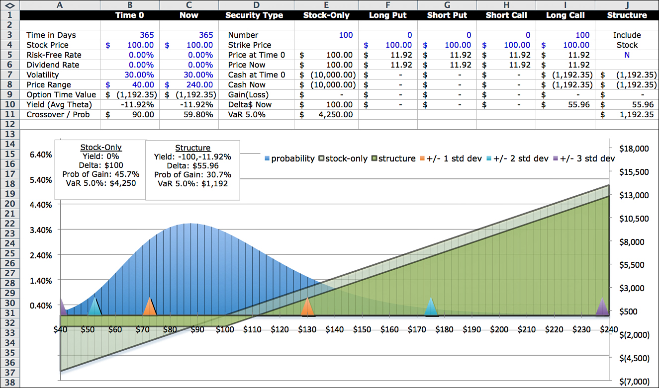
Crossover/Probability
Building a structured security is a process of reshaping the profit curve. Normally, this creates a single crossover point. The crossover point is the stock price where, on one side of the price, the stock-only position performs better, and on the other side of the price, the structure performs better. In this case, the crossover point is the lowest stock price at which a stock-only position has a higher value than the structured security being modeled.
In Figure 10.1, it is clear that the crossover point happens between $85 and $90. Because this is a simple structure, we can easily calculate the crossover exactly as $88.08, equal to the strike price of $100 minus the premium paid for the option of $11.92. In more complicated structures, it is convenient to have a general method of calculating the crossover price—and the probability that it will be exceeded. Figures 10.2a and 10.2b contain a sample format for determining the crossover point and the probability that the stock price will exceed the crossover. The columns also include the probability of a gain on the underlying security and the probability of a gain on the option. In terms of spreadsheet layout, the basic calculations of the model are performed in the Calc Engine and the Profit Calculator. The crossover/probability and other optional modules simply access and organize different aspects of the results.
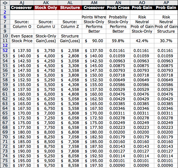
The first three columns of the Crossover/Probability module—the stock price in Column AJ, the stock-only profit in Column AK, and the structure profit in Column AL—are pulled in from the corresponding values in the Calc Engine and the Profit Calculator, as follows:
AJ13 = O13
AK13 = U13
AL13 = Z13
The next four columns answer these questions:
1. What are the stock price points where the stock-only profit is higher?
2. What is the probability of those points occurring?
3. What is the probability of a gain for the stock-only position?
4. What is the probability of a gain for the structure?
Column AM compares the stock profit to the structure profit and shows the points where the stock outperforms. The lowest number in the column is shown in Cell AM95 and on the display page as the crossover. Column AN is blank when Column AM is blank, and equals the probability of the point from the Calc Engine when Column AM is not blank. The sum of the probabilities are shown in Cell AN95 and on the display page as the probability of crossover. In this case, it is 59.8%. Column AO shows the probabilities of the points where the structure has a gain. This number is also shown as one of the four summary metrics in the text block inside the graph.
The probability that the stock price is equal to or above the crossover price is the sum of the probabilities for $90 and above. The probability that the stock will be profitable is 42.4% as shown in Cells AO95 and AO11. The probability that the structure will make a profit—that is, the probabilities of the stock price points above $111.92—is 30.67% as shown in Cells AP95 and AP11.
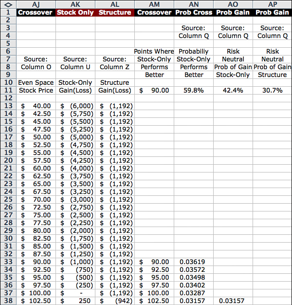
The Excel code for Columns AM through AP for Row 13 is:
AM13 = IF(AK13 >= AL13, AJ13, “ ”)
AN13 = IF(AM13 = “ ”, “ ”, Q13)
AO13 = IF(AK13 > 0, Q13, “ ”)
AP13 = IF(AL13 > 0, Q13, “ ”)
Copy these formulas down through Row 93, and insert the following formulas in Row 95:
AM95 = MIN(AM13:AM93)
AN95 = SUM(AN13:AN93)
AO95 = SUM(AO13:AO93)
AP95 = SUM(AP13:AP93)
I should point out a technical issue here. As mentioned earlier, the model uses “risk-neutral” probabilities. Risk neutral probabilities are calculated assuming no upward drift in the stock price. Over the longer term, it is often reasonable to expect an upward drift based on pricing models such as the Capital Asset Pricing or Arbitrage models. Over the shorter term, you may also have a view, using technical or fundamental analysis, that the trend is up.
In more advanced applications of the model (not covered in this book), it is possible to separate the risk-neutral probabilities calculated using the “risk-free rate” from probabilities using trend asssumptions. For instance, by assuming an expected return of 8% (but keeping the option pricing return assumption linked to the risk-free rate of zero), the probability of the option in this example producing a gain after one year is around 40% instead of 31%. With shorter option terms, the difference in the two methods narrows. And when the purpose is to compare a stock to a related structure, because both are being measured in the same way, the difference between the two is closer to the result using trend. As a practical matter, the main point is to be aware that probabilities associated with a single stock or a single structure may be understated over longer periods of time.
VaR 5.0%
The VaR, in this case, is equal to $1,192, the premium paid for the option. Although it is correct to say that, at the 5% tail boundary, the loss is $1,192, the concept of VaR is not as meaningful for a long option, where the loss is capped. In fact, the level of VaR doesn’t affect the answer within a wide range. The maximum loss occurs in Row 37 of Figure 10.2. The cumulative probability from Figure 8.3 for Row 37 is roughly 58%. VaR at the 58% level is also $1,192. This is an attractive aspect of long options. Your downside loss is capped fairly early, and one of the reasons commentators such as Jim Cramer who otherwise don’t recommend options for most investors sometimes recommend deep in-the-money call options as a stock substitute. (The reason for deep in-the-money call options instead of at-the-money or out-of-the-money is their relatively low time value premiums—that is, you don’t have to pay that much for time.)
Include Stock? Y/N
You might have noticed a new indicator in Column J. I included a switch that enables you to either include or exclude the stock component in Column E in the structure definition. If the entry in Cell J5 is N, the stock is not included and the structure is defined by the sum of Columns F–I. If the entry is Y, the stock component is included and the structure is defined by the sum of Columns E–I. For this chapter, the options are the only components of the structure, so the indicator is set to N. In the next chapter, covered calls are defined as a long stock position and a short call option position, so the indicator is set to Y in that case.
Short Call Option
Consider what happens when you sell a call option contract. In this case, you receive the premium of $1,192. The most you can make is $1,192 which happens if the stock price is below $100 at expiration. Losses occur at stock prices above $111.92, and because the stock price could conceivably go to infinity, the losses are unbounded. Figure 10.3 shows the profit curve.
If you sell a call option (short call option) and also have a position in the underlying stock, selling the option creates a covered call. If you don’t have a position in the underlying stock, it is an uncovered or naked call. Brokerage firms normally allow covered calls even for relatively inexperienced investors because the combined position is considered slightly more conservative than owning the stock by itself. On the other hand, to sell naked calls, you must apply for a higher level of options trading (for experienced option traders). This is because, with naked calls, there is the potential for large, even unlimited losses because there is no cap on how high a stock can go.
Option Time Value
Because there is no intrinsic value of this option, the entire premium consists of time value. But instead of paying for time, as with the long call option, you are being paid for time. If the stock price at expiration is equal to its value today of $100, you will have earned $1,192 as the time value goes to zero over the term of the option.
One of the most interesting aspects of options is the capability to generate yield by time decay. Regardless of how the stock price moves, time value goes to zero over the life of the option. Because this source of return is dependent only on the passage of time and not on the direction of the underlying security, it can be compared to the other time-related sources of investment return. Theta is to options what interest is to fixed income and dividends are to equities. And the potential return from theta is much higher than either interest or dividends.
Going back to the example, assume that the portfolio allocation to the stock is $10,000. When you sell the option, you get $1,192, so the net investment is $8,808. If the option expires out of the money (the stock is below $100), the return can be calculated as $1,192 ÷ $8,808 = 13.5%.
Returns from theta are higher with higher volatilities, and annualized returns are higher with shorter option terms. One- and two-month options significantly increase the potential yields compared to annual options due to the rapid time decay during that time.
Delta
Delta for a short option is opposite that of a long option, meaning that the short option value moves in the opposite direction of the stock price. The interpretation of delta is still the same and represents an equivalent number of shares of the stock, at least within a narrow range of stock prices.
Long Put Option
Figure 10.4 illustrates the profile and metrics of a long put option.
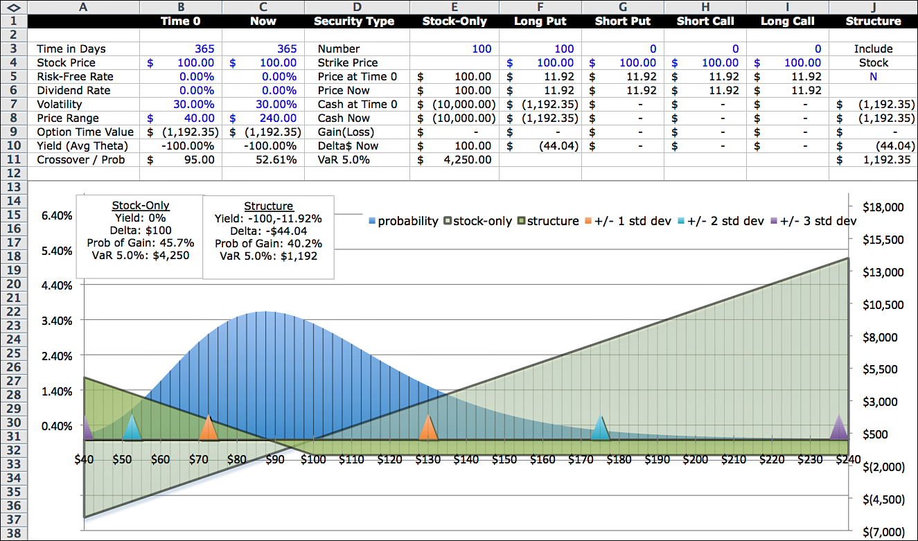
Long put options are often used as insurance. In concept, there is no difference between a homeowner’s policy that protects a house against fire and other damage, and a put option that protects a stock position against losses. Most people accept the idea that paying for homeowner’s insurance is prudent. However, very few investors use put options for portfolio insurance because of the cost. A typical homeowner’s policy costs less than 1% of the value of the house. Under these assumptions, the put option costs around 12% of the value of the stock. (One of the challenges for investors who want to use put options for insurance is finding ways to finance the put option at lower cost.)
VaR is $1,192, the same as with a long call option. The difference is that the loss happens at higher stock values. As with the long call option, VaR looses most of its relevance because of the shape of the curve. Notice that the loss is the same at $100 and $240. So it is technically correct to say that VaR at the 5% level is $1,192, and it is also true that VaR at much higher levels is also $1,192. When thinking about risk, it is more useful in this situation to use the maximum loss.
Short Put Option
Figure 10.5 illustrates the investment profile of a short put option.
Short put options are an alternative way to get exposure to a security. A short put option produces gains at higher stock prices and losses at lower stock prices. Because the profits from a short put option move in the same direction as a stock position, delta is positive. By selling put options, you can increase your exposure to a stock. Short puts are useful instruments for experienced traders to adjust both risk and return metrics.
If you are not familiar with short puts and would like to see some examples of short put options and their payoffs, there is an introductory video at Khan Academy. The link is www.khanacademy.org/finance-economics/core-finance/v/put-writer-payoff-diagrams.
Short put options are also helpful in financing partial protection as one leg of a put spread. You create a put spread by buying a put option at one strike price and selling a put option at a lower strike price. As an example, if you wanted to buy full protection on the stock in the example currently trading at $100, it would cost $1,192, or 11.92%. However, if you are satisfied with partial protection, such as covering only the first $10 in price drop, you could establish a put spread by buying the $100 strike put and selling the $90 strike put. The $90 strike put price is about $7. So the cost of insuring against a $10 drop in price is about $5 ($11.92 − $7). You have less protection, but the cost is less, too. To see the effect of this trade in the model, enter 100 shares and a $90 strike price in the short put column.
The yield on a short put option can be interpreted in different ways, depending on how you are using it. If it is a purely speculative bet, you stand to make 100% if the stock price at expiration is above the strike price. The chances of making some level of profit is 59.8%, using the model’s risk neutral probabilities. In terms of yield, if the allocation to the position is $10,000, the potential return is a $1,192 gain on a net investment of $8,808, or 13.53%. Of course, the actual yield is determined by the stock price at expiration. This definition of yield is average annualized theta, based only on time decay of the option, which assumes a stock price at expiration of $100.