
This chapter covers a number of ways to make choices about the appearance of a plot, some grouping and calculation tools, creating automatic functions for a specific class of objects, and creating object-oriented prototype functions. The chapter is split into three sections.
The first section gives an overview of the scale_, coord_, and guide_ functions along with related functions. The second section covers functions that cut data vectors into levels, summarize data vectors, and facet data vectors by faceting variables. The third section goes over functions to save, plot, print, and automate plots – as well as creating object-oriented prototypes.
10.1 Working with the scale_, coord_, and guide_ Functions
This section starts with, first, a subsection covering the scale_ functions, which affect the color, size, shape, and line type around and within a plot. The scale_ functions set up scales for properties that affect the appearance of the points and lines of a plot and, also, can set the properties of the legends associated with the scales.
The second subsection tells how to control the order of application for the functions that affect appearance. The third subsection is about formatting axes, with both scale_ and coord_ functions. The fourth subsection goes over the guide_ functions, which let the user set up a preset format that includes more than one formatting function.
10.1.1 The Scale Functions That Affect Color, Size, Shape, and Line Type
The scale functions set up a scale of values that affect the transparency, color, fill color, size, shape, or line type of points and lines. The names of the scale functions take the form of scale_ followed by the name of a characteristic (alpha, color, colour, fill, linetype, shape, radius, or size), usually followed by qualifiers.
Scales are usually applied to groups of points or lines but can be applied to ungrouped data. For numeric data, whether by groups or not, the types of scales available are plain scales or binned scales. For binned scales, the numeric data is binned, and the binned attributes are plotted. For categorical data – whether a factor object or a character object – only discrete scales are available. (Factor objects can be converted to numeric objects by the function as.numeric().)
For many of the functions in the ggplot2 package, the functions do not have a help page. Instead, the help page for the function is that of another function, which gives the arguments of the function. For example, scale_alpha_date() opens to the help page for scale_alpha() (and some other scale_alpha_ functions that do not include scale_alpha_date()). However, scale_alpha_date() is a function and can be called if the scale is for a vector of the Date class. Only functions with help pages are covered in this book.
Two qualifiers that most of the preceding characteristics use are identity and manual. The characteristics alpha, color, colour, fill, linetype, shape, and size have scale functions for the qualifiers identity and manual.
Note that, to use an aesthetic argument in a scale function, the group argument and/or a characteristic argument(s) must be set to a variable in an aesthetic function. The aesthetic function must be within the call to the preceding geometry or statistic function. The group argument and/or characteristic argument(s) should not be set in ggplot().
10.1.1.1 The Identity Qualifier
The identity qualifier tells the preceding geometry or statistic function to interpret the value of the characteristic argument without changes. For scale functions with the alpha, linetype, shape, and size characteristics, there are two arguments to the scale function with the identity qualifier, … and guide. For functions with the colour and fill characteristics, there are three arguments to the function, …, guide, and aesthetic.
The argument … is for arguments to the function discrete_scale() or continuous_scale(). See the help pages for the two functions for lists of the arguments of the functions. The arguments are not covered here.
The argument guide gives the name of the guide to be used by the scale (see Section 10.1.4). The default value of guide is “none” for the scale functions with the preceding six characteristics.
The argument aesthetics gives the kind of aesthetic on which to apply the color, colour (or color), or fill. There are four possible values for aesthetics: “colour”, “fill”, c( “colour”, “fill” ), and c( “fill”, “colour” ).
If both color and fill are set in the aesthetic function, both can be set in a color, colour, or fill scale function. For example, geom_point( aes( shape=shape, fill=shape-19, color=shape-17 ) ) + scale_shape_identity() + scale_fill_identity( aesthetic=c( "color", "fill" ) ) sets both the color and fill for the shapes 21–24. Here, the variable shape is an integer vector containing values between 21 and 24, inclusive.
For the scale functions with the color (or colour) characteristic, the aesthetic argument takes the default value of “colour”. For fill, aesthetic takes the default value of “fill”.
10.1.1.2 The Manual Qualifier
The scale functions with the manual qualifier create scales manually. The scale functions with the alpha, linetype, shape, and size characteristics and the manual qualifier have three arguments. The arguments are …, for arguments to the function discrete_scale(); values, for the values that make up the scale; and breaks, for the break points or levels of the scale.
On the help page for the functions with the manual qualifier (which the functions share and from which the information here is taken), the arguments of discrete_scale() are listed and described. The arguments are not covered here.
The values argument gives the values of the characteristic to be associated with each level or break class of the grouping variable. The argument takes a vector of the kind that the characteristic takes. The length of the vector is the number of classes in the grouping variable. There is no default value for values.
Formally, the elements of the values argument can be named, where the names are explicitly character strings. The character string must contain the character strings associated with the grouping classes. (Note that, in an aesthetic function, the grouping variable cannot be numeric.) For example, geom_line( aes( linetype=cut( dpi, 2 ) ) ) + scale_linetype_manual( values=c( "(85,2.05e+03]"="dotted", "(2.05e+03,4.01e+03]"="dashed" ) ) assigns the names of the two cut classes to two different line types.
The breaks argument gives information as to whether to plot a legend and, if a legend is printed, which grouping classes to include in the legend. The argument takes the value NULL, waiver(), or a character vector containing all or a subset of the character strings associated with the grouping classes. The argument can, also, take a function that creates the character vector, but the match between the grouping class character strings and the results of the function must be exact.
If breaks is set equal to NULL, no legend is plotted. If breaks is set equal to waiver(), a legend is plotted, and all of the grouping classes are included. If breaks is set equal to a character vector (or a call to a function that creates a character vector) of grouping class character strings, only the grouping classes with strings present in the vector are included in the legend. The default value of breaks is waiver().
10.1.1.3 The Alpha Characteristic
The functions, other than those with the qualifier identity or manual, for the characteristic alpha are the function with no qualifier and the functions with the continuous, binned, discrete, and ordinal qualifiers. All of the functions, except scale_alpha_discrete(), take two arguments, … and range. The discrete function takes one argument, ….
According to the help page for the preceding alpha scale functions, the … argument takes the arguments to the continuous_scale(), binned_scale(), or discrete_scale() function, depending on which scale function is run. See the help pages for the three functions for a list and description of the arguments.
The range argument takes a numeric vector of length two. The values of the elements must be between 0 and 1, inclusive, and give the range of the transparencies of the color(s) used to plot the shapes or lines. The value of 0 gives total transparency and of 1 gives total opacity. The default value of range is c(0.1, 1) for the four functions that use range.
10.1.1.4 The Color, Colour, and Fill Characteristics: Introduction
The scale functions, other than those with the identity and manual qualifiers, with fill, color, or colour for a characteristic are the scale functions with the continuous, hue, gradient, gradient2, gradientn, steps, steps2, stepsn, brewer, distiller, fermenter, grey, viridis_c, viridis_b, and viridis_d qualifiers. The color scales come in three versions, un-binned continuous scales, binned continuous scales, and discrete scales. Un-binned continuous scales have a continuous color bar for a legend by default. Binned continuous scales have a continuous bar with steps of color by default. Discrete scales have a legend with separate keys by default.
10.1.1.5 The Color, Colour, and Fill Characteristics: The Continuous Qualifier
For scale_colour_continuous() and scale_fill_continuous(), the functions work with numeric (continuous) data. The functions have two arguments, … and type. The argument … takes arguments to the continuous_scale() function. (See the help page for continuous_scale() for more information.)
From the help page for scale_colour_continuous(), the type argument takes the value “gradient”, “viridis”, or any function that returns the name of a continuous color scale. The default value of type is getOption("ggplot2.continuous.colour", default="gradient") for the colour characteristic and getOption("ggplot2.continuous.fill", default="gradient") for the fill characteristic.
10.1.1.6 The Color, Colour, and Fill Characteristics: The Hue Qualifier
The scale_colour_hue() and scale_fill_hue() functions create discrete scales, rather than continuous scales, and work with factor or character vectors. The functions take eight arguments: …, for arguments to discrete_scale(); h, for a hue range; c, for a chroma level; l, for a luminance level; h.start, for a beginning value for the hue; direction, for the direction to take around the color wheel; na.value, for the color value to use for missing values; and aesthetics, for the type of aesthetic to color. (See Section 3.4.1.3 for a description of hue, chroma, and luminance, under the functions hsv() and hcl().)
The h argument takes a two-element numeric vector. The first value is the smallest value of the range of hues, and the second value is the largest value. The values that R uses are between 0 and 360, inclusive; however, the values that are entered for the range limits are reduced modulus 360, that is, a range of 15–375 goes in a circle from 15 back to 15. (Note that the hue scale is circular rather than linear, that is, the scale comes back to the starting color over a range size of 360.) The default value of h is c(0, 360) + 15 for both functions with the hue qualifier.
The c argument takes a one-element nonnegative numeric vector. According to the help page for the hue functions, the possible values depend on the values for the hue and luminance. The default value for the two hue functions is 100.
The l argument takes a one-element numeric vector with a value that is between 0 and 100, inclusive. The default value for the two hue functions is 65.
The h.start argument takes a one-element numeric vector. The default value is 0 for both hue functions.
The direction argument takes a one-element numeric vector. The value must be either 1 or -1. If set to 1, the hues are chosen in the counterclockwise direction around the color wheel. If set to -1, the direction is clockwise. The default value for direction is 1 for both hue functions.
The na.value argument takes a one-element color value vector (see Section 3.4.1 for kinds of color values). The default value of na.value is “grey50” for both hue functions.
The aesthetic argument behaves the same as in the identity scale function for colour and fill (see Section 10.1.1.1). The default values are “colour” for the colour hue function and “fill” for the fill hue function.
10.1.1.7 The Color, Colour, and Fill Characteristics: The Gradient Qualifiers
The scale functions with the fill, color, and colour characteristics and the gradient, gradient2, and gradientn qualifiers are used with continuous variables. The functions have seven, nine, and eight arguments, depending on whether the qualifier is gradient, gradient2, or gradientn. The nine functions share five arguments. The five arguments are …, for arguments of the function continuous_scale(); space, for the color space; na.value (see Section 10.1.1.5); guide, for the name of the guide to use; and aesthetics (see 10.1.1.1).
The space argument takes only one possible value. The value is “Lab”. According to the help page for the nine functions, other color spaces are deprecated.
The guide argument takes a one-element character vector. Only two values are possible, “colourbar” for a continuous scale and “legend” for a discrete scale. The default value is “colourbar” for the nine functions.
The functions with the gradient qualifier also take the arguments low and high, for the colors at the ends of the scale. The arguments take a color value vector of length one. The default values for low and high are "#132B43" and "#56B1F7", respectively, that is the scale goes from a dark navy blue to a clear mid-blue.
The functions with the gradient2 qualifier take the arguments low and high, along with the argument mid, for the color of the middle of the scale. The default values of low, mid, and high are muted("red"), "white”, and muted("blue”), respectively.
The three gradient2 functions also take the midpoint argument, for the midpoint of the scale – measured in the units of the variable for which the scale is created. The default value of midpoint is 0.
The functions with the gradientn qualifier also take the colours (or equivalently colors) argument, for the colors to be used in the scale, and the values argument, for – according to the help page for the functions – the distance along a continuum from 0 to 1 of each color in colours.
The colours (or colors) argument takes a vector of color values of arbitrary length (see Section 3.4.1 for information about color values). The colors are used to generate a continuous scale. There is no default value for colours (or colors).
The values argument takes the value NULL or a numeric vector of unique values of the same length as colours (or colors). The values must be between 0 and 1, inclusive. The default value for values is NULL.
10.1.1.8 The Color, Colour, and Fill Characteristics: The Step Qualifiers
The scale functions that have the colour, color, and fill characteristics and that have the steps, steps2, and stepsn qualifiers create scales in binned steps. The functions are for continuous variables.
The arguments to the nine step functions are the same as the respective arguments to the nine gradient functions. The arguments also take the same default values as the nine gradient functions, except that the default value for guide is “coloursteps” in the nine step functions.
10.1.1.9 The Color, Colour, and Fill Characteristics: The Brewery Qualifiers
The scale functions that have the colour, color, and fill characteristics and that have the brewer, distiller, and fermenter qualifiers share a help page. The three functions that have the brewer qualifier are for discrete variables. The six functions that have the distiller and fermenter qualifiers are for un-binned continuous and binned continuous variables, respectively.
The brewer, distiller, and fermenter functions take five, nine, and seven arguments, respectively. The nine functions share five arguments. The arguments are …, for the arguments to the discrete_scale(), continuous_scale(), and binned_scale() functions, respectively; type, for the style of the scale; palette, for the color palette of the scale; direction (see Section 10.1.1.6); and aesthetics (see Section 10.1.1.1).
The type argument takes a character vector of length one. From the help page for the nine functions, the value of type must be one of “seq”, for sequential scales; “div”, for diverging scales; and “qual”, for qualitative scales (see the help page for a description of the three types). The default value of type is “seq” in the nine functions.
The palette argument takes either a one-element character vector or one-element numeric vector. For the character vectors, the character string is the name of the palette enclosed in quotes. The list of the names of the palettes is on the help page for the functions, under the section named “Palettes.” The palettes that are available by the integers depend on the value of type.
For type set equal to “seq”, 18 palettes are available, so the argument palette can take integer values from 1 to 18. For type set equal to “div”, nine palettes are available, so the argument palette can take integer values from 1 to 9. For type set equal to “qual”, there are eight palettes available, so palette can take integer values from 1 to 8. Any of the palettes can be accessed by setting the palette argument to the name of the palette enclosed in quotes. The choice does not depend on the value of type. The default value of palette for the nine functions is 1.
The direction argument has different default values for different qualifiers. For the brewer qualifier, direction is set to 1 by default. For the distiller and fermenter qualifiers, direction is set to -1 by default.
For the functions with the distiller qualifier, the four arguments not covered in the preceding text are values, space, na.value, and guide – which are covered in Sections 10.1.1.6 and 10.1.1.7. The arguments values, space, and na.value take the same defaults as in the gradient scale and hue scale functions. The argument guide takes the value “colourbar”.
For the functions with the fermenter qualifier, the two arguments not covered under the brewer qualifier are na.value and guide – covered in Sections 10.1.1.6 and 10.1.1.7. The default value for na.value is the same as in the preceding value, and the default value for guide is “coloursteps”.
10.1.1.10 The Color, Colour, and Fill Characteristics: The Grey Qualifier
The functions scale_colour_grey() and scale_fill_grey() work with discrete data (character or factor data) and create scales in shades of gray. The functions take five arguments. The arguments are …, for arguments to discrete_scale(); start and end, for the start and end values of the gray scale; na.value (see Section 10.1.1.6); and aesthetics (see Section 10.1.1.1).
The start and end arguments take one-element numeric vectors. The values must be between 0 and 1, inclusive. The smaller the value is, the darker the shade of gray is. The default values of start and end are 0.2 and 0.8, respectively.
The na.value argument takes the default value of “red” in the two grey functions. The aesthetics variable behaves as the argument behaves in Section 10.1.1.1.
10.1.1.11 The Color, Colour, and Fill Characteristics: The Viridis Qualifiers
The functions with the characteristics colour, color, and fill and the qualifiers viridis_c, viridis_b, and viridis_d are used for continuous un-binned scales, continuous binned scales, and discrete scales, respectively. The color scales, of which there are five versions for each of the nine functions, are suitable for many persons who cannot see some colors (have color blindness) because the scales work as well as gray scales as the functions work as colored scales.
The viridis_c functions and viridis_b functions take the same 11 arguments. The viridis_d functions take seven arguments – which are shared with the viridis_c and viridis_b functions.
The first seven arguments are …, for arguments to the continuous_scale(), binned_scale(), and discrete_scale() functions, depending on which viridis function is chosen; alpha, for the level of transparency; begin, for the beginning level of the scale; end, for the ending level of the scale; direction (see Section 10.1.1.6); option, for the color scheme; and aesthetics (see Section 10.1.1.1).
The alpha argument takes a numeric vector of length one. The value must be between 0 and 1, inclusive. The default value of alpha is 1.
The begin and end arguments take numeric vectors of length one. The values must be between 0 and 1, inclusive. The default values of begin and end are 0 and 1, respectively.
The direction argument is described in Section 10.1.1.6. The default value for the nine viridis functions is 1.
The option argument takes a character vector of length one. The character vector can either be a capital letter or a name. From the help page for the viridis functions, the possible values are “A” or “magma”, “B” or “inferno”, “C” or “plasma”, “D” or “viridis”, and “E” or “cividis”. The default value of option is “D” for the nine viridis functions.
The last four arguments for the functions with the viridis_c and viridis_b qualities are values, space, na.value, and guide, which are covered in Sections 10.1.1.6 and 10.1.1.7. The default values for values, space, and na.value are NULL, “Lab”, and “grey50”, respectively. The default values for guide are “colourbar” for the viridis_c functions and “coloursteps” for the viridis_b functions.
10.1.1.12 The Line Type Characteristics
The line type scale functions, other than the line type function with the identity and manual qualifiers, are scale_linetype(), scale_linetype_continuous(), scale_linetype_binned(), and scale_linetype_discrete(). The functions scale_linetype_continuous() and scale_linetype_binned() require numeric data. The function scale_linetype_discrete() requires discrete data.
According to the error message returned when attempting to set linetype to a continuous object in geom_line(), geom_path(), geom_curve(), and geom_segment(), linetype cannot be set equal to numeric data in an aesthetic function. If geom_line() and geom_path() are run with the preceding scale functions, the functions return an error.
If geom_segment() and geom_curve() are run with scale_linetype() or scale_linetype_continuous(), an error is given. If run with scale_linetype_binned(), the functions run, but the line types cannot be set. (To set the line types, use scale_linetype_identity().)
The functions scale_linetype() and scale_linetype_discrete() give the same result for discrete data. The functions can be used to set up the legend format for discrete (character or factor) variables.
The functions scale_linetype(), scale_linetype_binned(), and scale_linetype_discrete() take the same arguments. The arguments are …, for arguments to the discrete_scale() function, and na.value, for the value given to missing values. The default value of na.value is “blank” for the three functions.
10.1.1.13 The Shape Characteristics
The scale functions with the shape characteristic, other than the shape functions with the qualifier identity or manual, are scale_shape() and scale_shape_binned(). The functions are used to assign shapes (symbols) to points. The function scale_shape() works with discrete data. The function scale_shape_binned() works with numeric data.
There are 25 shapes available to the functions associated with plot() (the integers that can be assigned to pch). There are ways to use any of the 25 symbols in the ggplot2 functions. (For example, geom_point( aes( shape=( 1:25 )[ cut( dpi, 25 ) ] ) ) + scale_shape_identity() can be used to plot 25 levels of dpi for the 50 points in the LifeCycleSavings dataset. Single letters can be used in the same way.) However, by default, the ggplot2 functions only use six shapes, with two versions for the first three shapes – solid and outlined. The shapes are circles, squares, triangles, crosses, squares with a diagonal cross inside, and asterisks.
Both functions take the same two arguments. The arguments are …, for arguments to the function discrete_scale(), and solid, for whether to plot the circles, triangles, and squares as a solid color or as an outline.
The argument solid takes a logical vector of length one. If set to TRUE, a solid symbol is plotted. If set to FALSE, the shape is outlined. The default value of solid is TRUE.
10.1.1.14 The Size and Radius Characteristics
The scales for the size and radius characteristics affect the sizes of points and lines. There are five scale functions with the size or radius characteristic: scale_radius(), scale_size_area(), scale_size(), scale_size_binned_area(), and scale_size_binned(). The scale function with the radius characteristic sizes linearly. The scale functions with the size characteristic scale by area (proportional to the square of the radius). The five functions work with numeric data (continuous data).
The difference between scale_size_area() and scale_size() is that scale_size_area() scales so that a value of 0 scales to zero area. The scale_size() function does not. The functions with the binned qualifier create bins for the data before plotting the points or lines. (The preceding information is from the help page for the five functions – which the functions share.)
The scale_radius() and scale_size() functions have the same seven arguments with the same default values. The scale_size_binned() function has two more arguments and has one different default value. The scale_size_area() and scale_size_binned_area() functions have two arguments, both the same in both functions, including the same default value for the second argument.
The seven arguments for the first three functions are name, for the title of the legend if there is a legend; breaks, for the class levels in the legend; labels, for the class level labels in the legend; limits, for the lower and upper limits of the legend; range, for the range of point or line sizes in the plot and legend; trans, for the transformation to be applied to the data; and guide, for the style of the scale in the legend.
The name argument takes one of the values NULL, a character vector of arbitrary length, and a function that returns a valid object. If name is set to NULL, no title is plotted. If a character vector, only the first element is used. The default value of name in the preceding three scale functions is the waiver() function, that is, the value to which the argument size is set, if size is the first or only aesthetic set.
The breaks argument takes one of NULL, a numeric vector of arbitrary length, the waiver() function, and a function that takes the limits (see in the following) and returns break points. If the value is NULL, no legend is plotted. If the value is a numeric vector, the numbers are with respect to the values that size is set to in the aesthetic function. If some of the breaks are outside the range of the data, the keys or bin borders associated with the breaks do not plot – unless the limits argument (see in the following) is set and the breaks are within the limits set by the argument. The default value of breaks is waiver() in the first three scale functions, that is, R chooses breaks based on the value of the argument trans (see in the following).
The labels argument takes one of NULL, the waiver() function, a character vector of the same length as breaks, and a function that takes the value of breaks and returns a character vector of labels. For the first three scale functions, the default value of labels is waiver(), that is, R calculates good labels based on the value of trans.
The limits argument takes one of NULL, a two-element numeric vector, and a function that accesses the default limits and uses the default limits to create new limits. If set to NULL, the default limits are used. If set to a numeric vector, the two values give the lower and upper limits of the scale. The value NA can be assigned to a limit to use the current value of the limit, according to the help page. For the preceding three scale functions, the default value of limits is NULL.
The range argument takes a two-element numeric vector. The numbers give the smallest and largest sizes for the points or lines that are scaled. For the preceding three functions, the default value of range is c(1, 6).
The trans argument takes a one-element character vector or a transformation object for a value. According to the help page for the size and area functions, a transformation object is a function that uses a transformation, such as exponentiation, and the inverse of the transformation, to create a vector of breaks and labels.
If the trans argument is a character vector, the character vector must contain the name of a transformation, such as “log10” or “exp”. A transformation object must exist for the transformation. (See the help page for the size and radius functions for a list of transformation names for which transformation objects exist, as well as the transformation object names. Transformation objects can also be found in the scales package.)
A new transformation object can be created with the function trans_new() in the scales package. The names of the transformation objects have the form transformation_trans, where transformation is the name of the transformation and trans is an extension.
The default value of trans is “identity” for the preceding three scale functions. The identity transformation makes no transformation to the data.
The guide argument takes either a one-element character vector or the output from a guide function (see in the following). The default value of guide for scale_radius() and scale_size() is “legend”.
The scale_size_binned() function takes two more arguments, n.breaks, for the number of bin breaks, and nice.breaks, for whether to create nice-looking break points (e.g., 1000 instead of 1002.06). The n.breaks argument is not always followed, unless the nice.breaks argument is set to FALSE.
The n.breaks argument takes either the value NULL or a one-element numeric vector. The default value of n.breaks is NULL, that is, the transformation object determines the number of break points.
The nice.breaks argument takes a one-element logical vector. If set to TRUE, nice-looking break points are found. If set to FALSE, break points are set by a simpler method – without concern for the look of the break points. The default value of nice.breaks is TRUE.
The scale_size_binned() function has a default value for guide that is different. The default value of guide is “bins”.
For the scale_size_area() and scale_size_binned_area() functions, the arguments are …, for the arguments of the continuous_scale() function, and max.size, for the maximum size of the points or lines. The default value of max.size is 6 for both of the scale functions.
10.1.2 Setting the Order of Evaluation
The after_stat(), after_scale(), and stage() functions can be used within geometric functions to set the order of the evaluation of aesthetic arguments. When one of the preceding functions is used, the aesthetic argument is set equal to the preceding function within the aesthetic function of the geometry function.
Most geometric functions make use of a statistic function. By using after_stat(), a variable created by the statistic function can be used in calculating the value of an aesthetic argument.
The after_scale() function can be used to calculate new values for aesthetic arguments based on aesthetic arguments that have already been set. An aesthetic argument can be used on both sides of the equation.
The stage() function allows for the scaling of an aesthetic in multiple ways, both (either) after the statistic function is done and (or) after the initial scaling is done.
According to the help page for the three functions, if after_stat() is used, only those arguments created by the statistic function or that are in the environment from which ggplot() is called can be used to create a value for the aesthetic argument. The variables in the data frame are not available. The after_scale() function can only use variables created by the application of the initial aesthetic or variables in the parent environment. For stage(), variables from the data frame can only be used in the first argument of the function.
Code showing an example of using after_scale() twice in one geometry function. Since two aesthetics are used for the variable, a warning is given when the code is run
Note that both the color and size of the line segments are based on the value of group. A warning is given that the two aesthetics are based on the equivalent scales.
An example of using stage() to set fill colors in a histogram is given
Note that the aesthetic to which stage is assigned is fill and that the fill color is lightened by using the alpha() function on fill. The aesthetic argument color is set to the same color at full strength. (The example is based on an example on the help page for the three functions.)
10.1.3 Formatting Axes with the Scale and Coordinate Functions, Plus Some
The scale functions for which the characteristic is x or y and the coordinate functions both operate on the axes of a plot. According to the help pages for the functions, the scale functions operate before the statistic function used by the geometry function is run. The coordinate functions operate after the statistic function is run. For a scatterplot, both give the same result except that the tick marks differ.
The x and y scale functions have the continuous, binned, discrete, reverse, log10, sqrt, date, time, and datetime qualifiers. The coordinate functions begin with coord_ and have the cartesian, fixed, flip, map, quickmap, munch, polar, sf, and trans characteristics.
10.1.3.1 The Scale Functions
The scale function with the continuous qualifier gives the usual scale for x or y aesthetics that are continuous (numeric and un-binned). The binned qualifier creates bins for continuous x or y aesthetics and plots the points at the center of the bins. The scale functions with the continuous and binned qualifiers only run with x and y aesthetics that are continuous. The scale function with the discrete qualifier runs on both continuous and discrete x and y aesthetics but does not provide axis ticks or axis tick labels for continuous aesthetics.
The scale function with the reverse qualifier reverses the order of the axis. The scale function with the log10 qualifier transforms the scale of the axis to a base 10 log scale and changes the plotted geometry accordingly. All values of x or y must be positive for the log10 qualifier. The scale function with the sqrt qualifier transforms the axis to the square root of the values in x or y and changes the plotted values accordingly. All values of x or y must be nonnegative.
The scale function with the date qualifier creates a scale with values that are dates. The x or y aesthetic argument must be of the Date class for the date scale function. The scale function with the datetime qualifier creates a scale with values for both dates and times. The aesthetic argument x or y must be of the POSIXct class.
The scale function with the time qualifier creates a scale with values of time. The x or y aesthetic must be numeric and is converted to the format of the hms class (that is hh:mm:ss, where hh is the hours, mm is the minutes between 00 and 59, and ss is the seconds from 00 to 59). The hms() function can be used to format numeric data to the hms class. The numeric data is interpreted as in seconds if no formatting is done. There is not upper limit for hours. The values can be negative.
10.1.3.2 The Coordinate Functions
The coordinate functions all affect both axes, except that the function coord_trans() can also affect just one axis. The functions transform the coordinates of the axes.
The coord_cartesian() function creates Cartesian (linear) coordinates. The function coord_fixed() gives a plot for which the units on the x axis are in a fixed ratio to the units on the y axis, independently of the size of the graphics device. The ratio is given by the ratio argument and is set to 1 by default.
The coord_flip() function flips the axes. The coord_map() and coord_quickmap() functions create coordinates of longitudes and latitudes. Three of the six arguments for the map characteristic functions are projection, for the type of map projection; xlim, for the longitudinal limits; and ylim, for the latitudinal limits, assuming the usual orientation.
The coord_polar() function uses polar coordinates. Three of the four arguments to the function are theta, for which of x or y to use for the angle; start, for the starting angle in radians, with 0 at the top of the plot; and direction, for the direction to go around the plot – the value of 1 for clockwise and -1 for counterclockwise.
The transformation to polar coordinates plots the relative sizes of variable assigned to theta through 360 degrees and ignores the absolute sizes of the values, except for the numbers in the labels. The other variable gives the radius for each value in theta.
The coord_sf() function creates coordinates for simple feature data. Simple features are spatial data.
According the help page for coord_munch(), the function is used within geometry functions. The function breaks the coordinates on the axes into small pieces for cleaner vector plotting.
The coord_trans() function provides for manual transformation of one or both axes by a function. The argument(s) x and/or y are set equal to a function name(s) in quotes or a transformation object(s). The transformation can be user generated. See Section 10.1.1.14 for more information about transformation names and transformation objects.
10.1.3.3 Other Axis Functions
There are a few other functions that affect axes. The xlab() and ylab() functions can be used to manually set axis labels. The lims(), xlim(), and ylim() functions can be used to set limits for an aesthetic variable or axis. The expansion() and expand_scale() functions are used as values for the expand argument in scale functions. The functions calculate the axis limits needed to put an area of a given size between the axes and the plot.
The dup_axis() and sec_axis() functions are used as values for the sec.axis argument in x and y scale functions. The functions format a second axis opposite the original axis. The dup_axis() function duplicates the original axis. The sec_axis() function creates a new axis based on a one-to-one transformation of the scale of the original axis.
The xlab() and ylab() functions have one argument, label, for the character string containing the label. (The label can also be assigned in a scale function by setting the argument name.)
The lims() function takes named two-element vectors, where the name is of an aesthetic argument (e.g., x=c(5,20)). The vectors can be of the numeric, character, factor, Date, POSIXct, or hms class, depending on the class of the aesthetic argument. The vectors are separated by commas in the call to lims().
The functions xlim() and ylim() take two single numeric values giving the lower and upper limits of the x or y axis. The functions are for numeric (continuous) axes.
The expansion() and expand_scale() functions have the same arguments. The arguments are add, for the value to add to and subtract from the axes for the expansion area, and mult, for a multiplicative expansion factor.
The dup_axis() and sep_axis() functions have the same five arguments. The arguments are trans (see Section 10.1.1.14), name, breaks, labels, and guide. (See the help page for continuous_scale(), binned_scale(), or discrete_scale() for a description of the four arguments – which help page function depends on the type of scale.) The default value of trans is NULL in sec_axis() and ~. in dup_axis(). The default values of name, breaks, labels, and guide are waiver() in sec_axis() and derive() in dup_axis().
10.1.4 The Guide and Draw Key Functions
The guide functions are used to format properties of the axes or the key to the scaling variables (e.g., a legend or color bar). Most of the guide functions are used within scale functions. (The guide argument appears in the list of the arguments of continuous_scale(), binned_scale(), and discrete_scale().) The draw key functions give the style of the keys used in legends.
10.1.4.1 The Guide Functions
There are nine guide functions that are supported in the ggplot2 package and five that are not supported, but that exist. Of the nine functions, one function, guide_axis(), provides structuring for axes. Two are colour/color duplicates. Four structure the key to the scaling variables. The four are guide_legend(), guide_colorbar(), guide_colorsteps(), and guide_bins(). One function, guide_none(), gives no legend or no axis tick marks and tick mark labels. One function, guides(), combines more than one guide in one object.
The functions are set by setting the argument guide equal to either a name in quotes or the full function (e.g., guide=“bins” or guide=guide_bins()), in a scale function. See the help pages for the guide functions for a list of the arguments to the functions.
The Guides That Affect Axes
The guide_axis() function has six arguments. The arguments set the axis label, what to do when axis tick labels overlap, the angle of the labels, the position of the axis by side, and the order in which the axis plotting is done.
The guide_none() can be used with the x and y scale functions. The function is used to assign an axis label without tick marks or tick mark labels. The axis label is assigned to the title argument. The position of the label can be specified with the position argument, by setting the argument to “bottom”, “left”, “top”, or “right".
The Guides That Affect the Key to the Scaling Variables
The guide_none() function can be used to suppress the key to the scaling variable when used with the scale functions that are not axis scale functions. The guide_legend() function sets up a legend with keys for the scaling variable (which is usually a function of the aesthetic arguments). The guide_bins() function sets up a strip of distinct steps with levels shown at the intersections of the steps. The steps are keys within blocks. The function guide_colorsteps() is a version of guide_bins() with keys that are rectangles filled with the colors of the scale. The three functions can be used with un-binned continuous (numeric) data, binned continuous (numeric) data, and discrete (character or factor) data.
The guide_colorbar() function can only be used with continuous data (un-binned or binned). For un-binned continuous data, the function plots a continuous graded color scale. The scale is labeled with increasing or decreasing levels of the scaling variable. For binned scales, guide_colorbar() behaves like guide_colorsteps().
An example of code for setting up a set of guides using the function guides()
In the listing, the guides are first assigned to an object named gd. After the plot is set, the guides are run by including the name gd after the geometry function. Note that the guides are not set within a scale function.
10.1.4.2 The Draw Key Functions
There are 16 draw key functions. The names of the functions start with draw_key_, which is followed by the name of a geometry. The geometry names available are point, abline, rect, polygon, blank, boxplot, crossbar, path, vpath, dotplot, pointrange, smooth, text, label, vline, and timeseries. (Note that vpath is not a listed geometry but is included in the list from the help page for draw_key, from where the information here comes.)
The key styles are automatically assigned by the geometry and statistic functions, but the default key style can be changed. The draw key functions are assigned to the key_glyph argument in the geometry and statistic functions. (The key_glyph argument is in the layer() function. The geometry and statistic functions all call the layer() function.)
The form of the assignation is either the geometry name in quotes or the total function name without the ending parentheses and not in quotes (e.g., key_glyph="abline" or key_glyph=draw_key_abline).
10.2 Functions That Cut, Summarize, and Facet
The cut functions discretize continuous (numeric) vectors. The facet functions plot several plots, where each plot contains the data associated with a value of a grouping variable. The summary functions give summaries of numeric vectors and can be done by groups. Most of the summary functions can be plotted on grouped (or ungrouped) data.
There are three cut functions in the ggplot2 package, three facet functions, and five summary functions. (The summary functions are based on functions in the Hmisc package and the dependencies of the Hmisc package.) There is also a function named resolution(), which gives the resolution (the smallest difference between different numbers) of a numeric vector.
10.2.1 The Cut Functions
The three cut functions in the ggplot2 package are cut_interval(), cut_number(), and cut_width(). The functions are based on the cut() function in the base function and can use the arguments of cut() as well as the arguments listed on the help page for the three functions. The first argument of the three functions is x, for the numeric vector to be cut into discrete factor levels.
The cut_interval() function cuts the range of the data into intervals based on either n, for the number of equal-length intervals, or length, for the length of the equal-length intervals. If the n argument is chosen, the width of the intervals is the range of the numeric vector divided by n.
If the length argument is chosen, the argument length does not necessarily divide evenly into the range of the data vector. The function determines the starting value for the intervals. Both n and length take a one-element numeric vector.
The cut_number() function has one argument, n, for the number of intervals. The function behaves like cut_interval() with the choice of n.
The cut_width() function provides more flexibility. The specified arguments, other than x, are width, for the width of the intervals; center, for the center of the first interval; boundary, for the beginning of the first interval; and closed, for whether to close the intervals on the left or right (closing a boundary means that a data point on the closed boundary of the interval is included in the interval).
The width, center, and boundary arguments take one-element numeric vectors. There is no default value for width. The default values of center and boundary are NULL.
The closed argument takes a one-element character vector, and the value must be “left” or “right”. The default value is “right”, that is, the intervals are closed on the right.
10.2.2 The Summary Functions and the resolution() Function
The summary functions in the ggplot2 package are used with the stat summary functions, that is, the functions that begin with stat_summary. The stat summary functions take the argument fun, to which the summary functions can be assigned. Four of the summary functions are based on functions in the Hmisc package, which must be installed for the functions to run, but need not be loaded. The functions are mean_cl_boot(), mean_cl_normal(), median_hilow(), and mean_sdl(). The fifth function is mean_se(). At the end of the section, the function resolution() is covered.
The summary functions all take two arguments: x, for the numeric vector to be summarized, and …, for the arguments to the function in the Hmisc package with the preceding names preceded by the letter s. The functions all return a data frame of length three. The names of the data.frame elements are y, ymin, and ymax.
The mean_cl_boot() and mean_cl_normal() functions give the mean of the data and confidence interval limits for the mean of the data based on bootstrapping the data or based on the normal distribution (using quantiles of the t distribution), respectively. The median_hilow() function gives the median of the data and the lower and upper empirical quantiles of the data based on the level of confidence. For the three functions, the level of the confidence interval is set by the argument conf.int and takes the value of 0.95 by default.
The mean_sdl() and mean_se() functions return the mean of the numeric vector, the mean minus a constant multiplier multiplied by the standard deviation of the vector or the standard error of the mean, and the mean plus a constant multiplier multiplied by the standard deviation of the vector or the standard error of the mean. For mean_sdl(), the standard deviation of the vector is used. For mean_se(), the standard error of the mean is used. The multiplier is set with the mult argument in both functions. By default, the value of mult is 2 for mean_sdl() and 1 for mean_se().
The code for the example in Figure 10-1 of using mean_cl_boot() in stat_summary()

An example of using mean_cl_boot() with stat_summary() and scale_x_binned() to plot summary statistics on a scatterplot within bins
In Figure 10-1, the code in Listing 10-4 is run. The summary statistics are in mid-gray.
Note that scale_x_binned() is used to bin the pop75 values. The mean and confidence intervals are of the pop15 values within each bin. The means and confidence intervals are in mid-gray. The plotted data points are black.
The resolution() function finds the resolution of a numeric vector. The resolution is the smallest difference between adjacent values within the vector. If two adjacent values are the same, the resolution is set to 1. The function resolution() takes two arguments: x, for the numeric vector, and zero, for whether to automatically include the value 0 in the vector.
The x argument takes a numeric vector of arbitrary length. The zero argument takes a one-element logical vector. If set to TRUE, a 0 is added to the vector. If set to FALSE, no 0 is added. The default value of zero is TRUE.
10.2.3 The Facet Functions
The facet functions create multiple plots based on applying a grouping variable or multiple grouping variables to vectors in a data frame. The data used in the plots are from the given data vectors, but no plot shares data with another plot, and all of the data in the vectors is plotted. There are three facet functions, facet_null(), facet_wrap(), and facet_grid().
There are also functions that are used to create values for arguments in the facet_wrap() and facet_grid() functions. The vars() function quotes the grouping variable(s) and behaves like the aes() function. The function is used with the argument facets in facet_wrap() and with the arguments row and col in facet_grid(). There are also functions used with the argument labeller (see in the following).
The facet_null() function is the function used to plot a single panel. The function is the function called by default when facet_wrap() and facet_grid() are not called. The function takes one argument, shrink, for whether to shrink the plot down to the dimensions of the output from the statistic function, if a statistic function is called, or the statistic function associated with the geometry function, if a geometry function is called. The default value of shrink is TRUE, that is, do the shrinkage.
The facet_wrap() function takes a vector of plots (the facets) and, by default, plots them from left to right. New lines are started as the function determines a new line is appropriate. The first argument is facets, for the one or more variables to be used for faceting the data. The value of the argument can take forms like vars( var1 ), “var1”, ~ var1, vars( var1, var2, var3 ), var2 ~ var1, ~ var1 + var2, c( “var1”, var2” ), and var3 ~ var1 + var2, where var1, var2, and var3 are the names of the faceting variables and are variables in the data frame or are expressions based on variables in the data frame. If the function labeller() is used, the variables that are expressions should be assigned a name.
The number of rows and/or columns can be specified, but there must be enough places for the total number of facet plots. Otherwise, an error occurs. The direction of plotting can be changed from left-to-right to top-to-bottom. The position of the facet plot labels can be changed from the top of each plot to any of the other sides of each plot.
The facet_grid() function creates a matrix of plots. The first two arguments are rows and cols, for the variables to put in the rows and columns. One or the other or both can be specified. The argument rows can take the same kinds of values as the argument facets in facet_wrap(). The argument cols must be set equal to NULL or variable name(s) and/or expression(s) enclosed by the vars() function parentheses and separated by commas.
The levels of the value of rows go down the columns, and the levels of the value of cols go across the rows. By default, the facet labels for the rows go to the right side, and the facet labels for the columns go across the top.
A choice can be made about whether the plots should be the same size, whether to switch the row and/or column facet labels to the bottom and/or left, and whether to plot margin plots. Row margins, column margins, or both margins can be plotted.
The functions facet_wrap() and facet_grid() share five arguments. The first of the arguments tells the function whether the scales should be the same for the plots and, if not, what should be allowed to vary. By default, the plot scales are the same. The second is shrink, covered under facet_null().
The fourth tells the function whether to treat the layout with the rows starting at the top and the columns at the left or to have the rows start at the bottom and the columns at the left. The default is that rows start at the top.
The fifth tells the function whether to drop row and column combinations for which there is no data. By default, combinations with no data are dropped.
The argument switch in facet_wrap() is soft deprecated and should not be used. The argument facets in facet_grid() is deprecated and should not be used.
The third argument, labeller, takes a function of the labeller class. The value that labeller takes is either the name of a function of the labeller class (unquoted and with no parentheses), a call to the function as.labeller(), or a call to the function labeller(). In labeller() the names of the faceting variables are assigned a function of the labeller class or a call to as.labeller(). The function labeller() is used to assign different labeling functions to different faceting variables.
There are six preset labeling functions (which start with label_) for formatting and setting panel labels. The extensions of the labeling functions are value, for using the values of the variable for labels; both, for using both the variable name and the values of the variable for labels; context, for using the value if there is one faceting variable and both the variable name and the value if there are more than one faceting variable; parsed, for using names generated with plotmath() as labels; bquote(), for assigning names generated by plotmath() to labels for rows and columns; and wrap_gen, for using the strwrap() function to wrap the label text.
The function as_labeller() is used to create new labeling functions. To assign facet labels that are different from the default labels, as_labeller() must be used. If there are more than one faceting variable on which to change the labels, more than one labeling function is created (see Listing 10-5).
When using as_labeller(), the format must be correct. The first argument, x, can be a function with the correct form or a vector of values of the factor variable converted to names and set equal to the character strings containing the new facet labels. For example, if the values of a factor variable named process are “fn” and “1rw” and the labels for “fn” and “1rw” should be “Finished” and “Raw 1”, then the expression c( fn="Finished", `1rw`="Raw 1") entered into as_labeller() as the value of x creates a function of the labeller class that gives the desired result. The labeller function created by as.labeller() is entered into labeller(). Note that, since “1rw” starts with a number, 1rw cannot be a legal name in R; however, `1rw` is a legal name. The backticks make the name legal.
Code for the example in Figure 10-2 of using facet_wrap(), vars(), as_labeller(), and labeller()
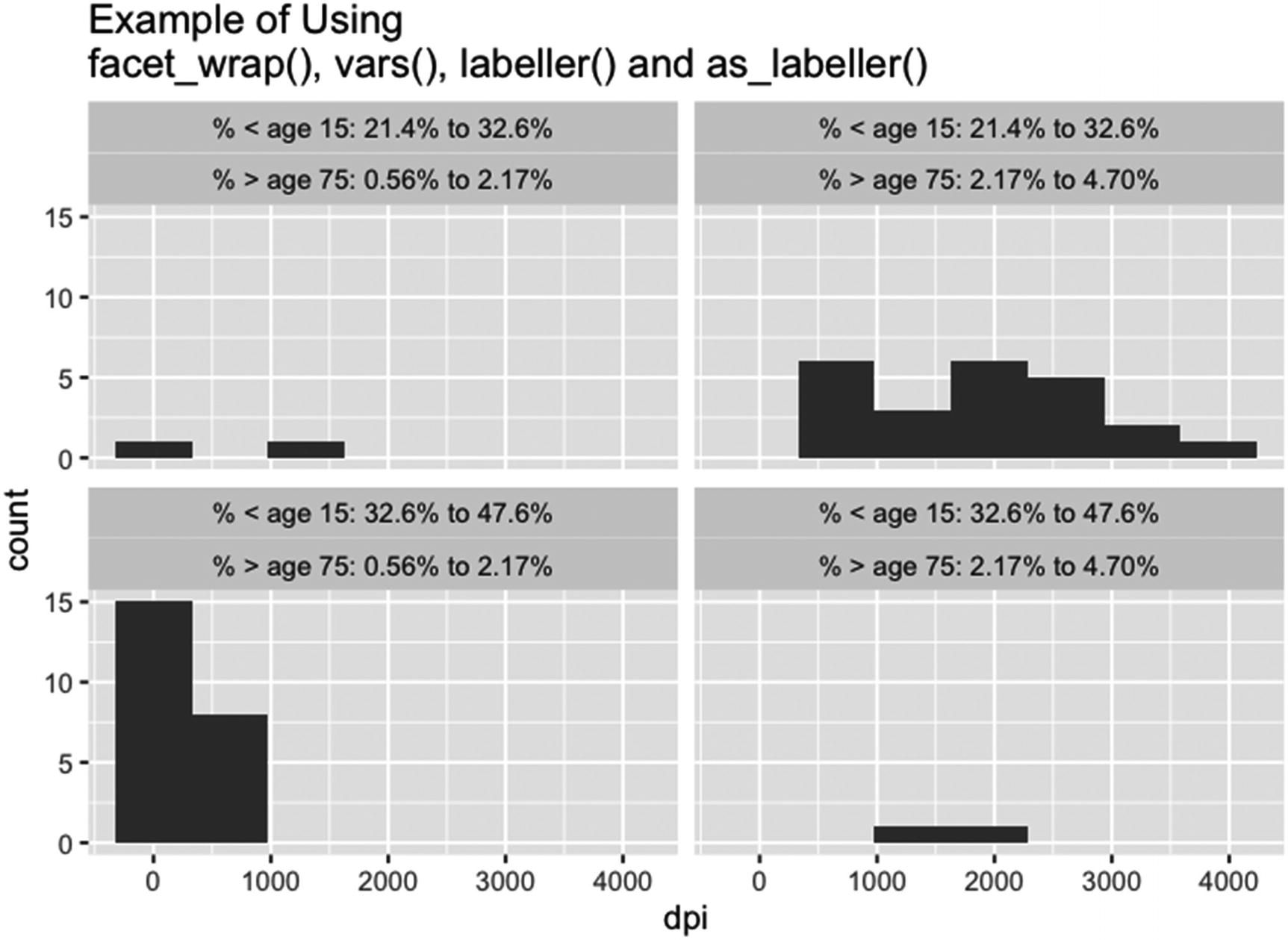
An example of using facet_wrap() with vars(), as_labeller(), and labeller()
In Figure 10-2, the code in Listing 10-5 is run.
Note that the labels are in the order that the faceting variables appear in the argument facets. Also, the first value of the first faceting variable stays the same as the values of the second faceting variable increase while the plots go from left to right. And the function creates a line break after the second plot, which creates a nice-looking figure. See the help pages for labeller() and as.labeller() for a list of arguments and more examples.
10.3 Working with Plots, Automatic Plots, and Prototypes
In this section, the functions that save, plot, and print plots are covered. Functions that create functions that automatically create a plot based on the class of the object(s) plotted are gone over. Last, the functions that create prototypes are described.
In Subsection 10.3.1, the functions ggsave(), plot() for ggplot objects, and print() for ggplot objects are covered. In Subsection 10.3.2, the functions auto_plot() and auto_layer() are presented. In Subsection 10.3.3, the functions used to create prototypes are given.
10.3.1 The ggsave() Function and the plot() and print() Functions Applied to ggplot Objects
The function ggsave() is a function that saves a plot to a file outside of R. The kind of graphics file created can be set by the extension given the file or by specifying the kind of device. The functions plot() and print(), when applied to ggplot objects, are useful when ggplot() is called within a function. Both functions, operating on an object of the ggplot class, create a plot.
The first argument of ggsave() is filename, for the file name to be assigned to the plot (enclosed in quotes). The file name does not include the path to where the file is to be saved, which is specified by the argument path (also enclosed in quotes) and which is the workspace by default.
The second argument of ggsave() is plot, for the plot to save. The argument plot, by default, saves the plot that is on the graphics device. Otherwise, plot can be assigned to the name of an object containing a plot generated by the ggplot() function or the code for the plot.
The third argument is device, for the kind of graphics format to use. The argument can be either the file extension in quotes or the name of the function that generates plots of the given extension, with the open and close parentheses (see Section 6.1 for a discussion of graphics devices and graphics formats). From the help page for ggsave(), the list of available extensions is “eps”, “ps”, “tex”, “pdf”, “jpeg”, “tiff”, “png”, “bmp”, ”svg”, and, on MS Windows devices, “wmf”.
The fourth argument is path, described in the preceding text under the first argument. There are seven more arguments, including the last argument, …, for the arguments to the graphics device function. The arguments give a scaling factor and the width, height, units, and resolution of the plot. By default, the scaling factor is 1, the width and height are given by the size of the graphics device, and the resolution is 300 dots per inch.
The tenth argument is limitsize, for whether to limit the size to 50 inches by 50 inches. According to the help page, the argument protects against the common mistake of using sizes in pixels rather than inches, centimeters, or millimeters. The default value of limitsize is TRUE.
The functions plot() and print() are used when ggplot() is run within a function (e.g., to create multiple plots by looping over datasets) If the usual aesthetic function is used, the functions give an error. See the introduction to Section 8.2 for the aesthetic functions that are used inside of functions calling ggplot().
If the correct aesthetic function is used and the ggplot() functions are run, but not within a plot() or print() function, then the functions run but the plots are not plotted. The plot() or print() function generates the plots externally.
10.3.2 The autoplot() and autolayer() Functions
The autoplot() and autolayer() functions are used to create a basic format for a class of objects. I think that once autoplot() (or autolayer()) is set for a class of objects within a workspace, when the class of objects is called in ggplot() (or layer()), the format in autoplot() (or autolayer()) is the starting format. So use with caution.
An example of setting autoplot() to plot objects of the ggplot class
Note that one of the classes of the object test.plot is ggplot. Also, the function autoplot() automatically determines that a method exists for objects of the ggplot class, so the ggplot extension is not used in the call to autoplot().
10.3.3 Prototype Functions in the ggplot2 Package
The ggplot2 package has a number of functions for creating and working with ggplot2 prototype functions. There are five functions associated with prototypes in the ggplot2 package, ggproto(), for creating prototype functions; ggproto_parent(), for accessing a parent function of a prototype function; is.ggproto(), for testing whether a function is a prototype function; and format() and print(), for the format() and print() methods used with the prototype function.
According to the help page for ggproto(), the function implements an object-oriented styled approach to programming in R. The approach gives functions that run quicker than other approaches in R and that work across packages.
The function ggproto() has three arguments, `_class`, for the class name to give to the objects which the prototype function creates; `_inherit`, for the object of the ggproto class from which the prototype function inherits; and …, for the named values that make up the prototype. The values can be any R object, including objects of the atomic types and functions.
The `_class` and `_inherit` arguments can be set to NULL and are set to NULL by default. The … argument contains the objects – usually variables and function definitions – that make up the prototype function. The objects are separated by commas.
A function definition can refer to the prototype function by using the argument self in the argument list of the function definition. The objects in the prototype function can then be referred to with the notation self$variable_name, where variable_name is the name of the object in the prototype function.
The variables set in the prototype function can be updated at each call to the prototype function by setting the variable self$variable_name – with variable_name being the name of the variable that is to be set – equal to an expression. The expression can contain self$variable_name; self$variable_name_other, with variable_name_other being the name of another variable set in the prototype function; and arguments in the argument list of the function definition.
The function ggproto_parent() has two arguments, parent, for the names of the parent prototype function, and self, to refer to the prototype function being defined. Neither has a default value.
According to the help page for ggproto(), a function defined in the parent prototype function is referred to with the expression ggproto_parent( parent_prototype_function_name, self )$defined_function_name, where parent_prototype_function_name is the name of the prototype function and defined_function_name is the name of a function defined within the prototype function. The arguments to the function that is defined in the parent prototype function are set within parentheses after the expression ggproto_parent( parent_prototype_function_name, self )$defined_function_name.
The function is.ggproto() takes one argument, x, for the object to be tested. If the object is of the ggproto class, TRUE is returned. Otherwise, FALSE is returned. There is no default value for x.
The help page for ggproto(), which is shared with ggproto_parent() and is.ggproto(), contains simple examples of using ggproto() and ggproto_parent(). The help page for register_theme_elements() contains a practical example of using ggproto().